


Introduction
Melting of the ice sheets covering Greenland and Antarctica is accelerating, presumably in response to rising global temperatures (Reference Wouters, Chambers and SchramaWouters and others, 2008; Reference Jiang, Dixon and WdowinskiJiang and others, 2010; Reference Rignot, Velicogna, Van den Broeke, Monaghan and LenaertsRignot and others, 2011; Reference ShepherdShepherd and others, 2012). Ocean forcing, where warm, saline (hence dense) water undercuts the deeper parts of marine-terminating glaciers (Reference Motyka, Hunter, Echelmeyer and ConnorMotyka and others, 2003), is believed to be an important aspect of accelerating ice loss on both land masses (Reference Payne, Vieli, Shepherd, Wingham and RignotPayne and others, 2004; Reference Shepherd, Wingham and RignotShepherd and others, 2004; Reference Holland, Thomas, de Young, Ribergaard and LyberthHolland and others, 2008; Reference StraneoStraneo and others, 2010, Reference Straneo2012; Reference Joughin, Alley and HollandJoughin and others, 2012; Reference Park, Gourmelen, Shepherd, Kim, Vaughan and WinghamPark and others, 2013). However, studying this process is challenging, as it involves measurements in or near the highly dynamic ice/ocean interface.
Breiðamerkurjökull is a large outlet glacier of Vatnajökull, Iceland’s main ice cap (Fig. 1). Aerial photography presented by Reference Björnsson, Pálsson and GuðmundssonBjörnsson and others (2001) suggests that the glacier retreated for most of the 20th century. The glacier has a mostly grounded ice front which calves into a 20 km2 tidal lagoon (Jökulsárlón) on the south side of the island, making it an excellent ‘natural laboratory’ for studying ice/ocean interactions (Reference Howat, Tulaczyk, Waddington and BjörnssonHowat and others, 2008). The lagoon has a maximum depth of 300 m and is connected to the North Atlantic Ocean through a 100 m wide by 20 m deep engineered channel lined with rip-rap (Reference BjörnssonBjörnsson, 1996).
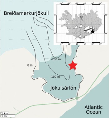
Fig. 1. Field site location (black star, inset). Radar location relative to the glacier (red star). Glacier locations taken from the Global Land Ice Measurements from Space (GLIMS) database (Reference SigurðssonSigurðsson, 2005; Reference Raup, Racoviteanu, Khalsa, Helm, Armstrong and ArnaudRaup and others, 2007). Black lines show approximate bed topography contours digitized from Reference Björnsson, Pálsson and GuðmundssonBjörnsson and others (2001).
In 2011, 2012 and 2013, we deployed a terrestrial radar interferometer (TRI) at Breiðamerkurjökull with four primary objectives: (1) to assess instrument performance; (2) to observe the influence of calving and tides on the instantaneous ice velocity; (3) to observe changes in ice mass, distribution and retreat from year to year; and (4) to assess the role of ocean currents in ice mass loss. The TRI is a newly developed technology with the potential to complement existing instrumentation for ice velocity measurements (Reference Riesen, Strozzi, Bauder, Wiesmann and FunkRiesen and others, 2011). In contrast to point measurements provided by GPS receivers, TRI provides a spatially continuous velocity field over tens of kilometers in extent and provides better temporal resolution (several minutes) than satellites, which have typical revisit times of several days or longer (Reference CovelloCovello and others, 2010; Reference Werninghaus and BuckreussWerninghaus and Buckreuss, 2010), without the need for dangerous and/or expensive in situ deployments on unstable glacier surfaces. TRI also provides high-quality digital elevation models (DEMs) to determine surface slopes and ice volume change, and can be used in an iceberg-tracking mode to infer surface currents.
Methods
Instrument description
The TRI used for this study is the GAMMA Portable Radar Interferometer (GPRI). The GPRI is an interferometric, Ku-band (1.74cm wavelength), real-aperture radar that provides high-resolution intensity images and is also sensitive to line-of-sight surface displacements of ∼1 mm (Reference Werner, Strozzi, Wiesmann and WegmüllerWerner and others, 2008). Two-dimensional velocities can potentially be determined with feature tracking.
The range resolution of the GPRI is 0.75 m, independent of distance, to a first approximation. The azimuth resolution of the GPRI at 1 km is 7.5 m, scaling linearly with distance. The radar has one transmitting antenna and two receiving antennas with a 25 cm baseline, and is positioned on a rotating frame (Fig. 2). The radar takes ∼90s to scan and prepare data from a 100° arc. Consecutive interferograms from one transmitting/receiving antenna pair are used to observe the velocity. The presence of two receiving antennas allows mapping of the glacial topography to a vertical precision of ∼3 m at 2 km distance (Reference Strozzi, Werner, Wiesmann and WegmullerStrozzi and others, 2012).

Fig. 2. A typical TRI field set-up at Breiðamerkurjökull. The top antenna transmits at Ku-band (1.74 cm wavelength) and the bottom two antennas receive the backscattered signal. The antenna mount scans in azimuth, in this area up to 100°. The calving front is ∼4 km away. Note icebergs in the foreground.
Data collection and analysis
We imaged the glacier with the TRI for a number of multi-hour periods over 3 days in September 2011, 4.5 days in August 2012 and 2 days in August 2013. Each year, we positioned the radar on moraine deposits 4 km away from the terminus in approximately the same spot. The location was easily accessible and provided a high vantage point to minimize interference from moving icebergs, while being close enough to the terminus to minimize atmospheric noise.
The radar scanned 50° arcs with a range 2–6.5 km in 2011, 90° arcs with a range 50 m–8.5 km in 2012 and 100° arcs with a range 50 m–16.9 km in 2013. Velocity maps were constructed using 3.5 hour periods of 1 min interferograms from 2011, and 3.5 hour periods of 3 min interferograms from 2012 and 2013.
Radar image processing was done using the GAMMA software. The resulting imagery was converted into rectangular (map) coordinates with 10 m pixel spacing. The TRI imagery was georeferenced by rotating the map coordinate data around the pixel containing the radar to produce the best visual match to a Landsat image.
Since the radar obtains high-precision displacement measurements via phase comparisons that are inherently ambiguous, the phase data must first be ‘unwrapped’ to investigate changes. Phase differences between successive images were unwrapped using a minimum-cost-flow algorithm (Reference CostantiniCostantini, 1998), and then converted into velocities. The radar images were multi-looked (averaged) in range by a factor of 10 to reduce noise.
Phase-unwrapped images were converted into line-ofsight velocity maps using
where v is velocity, λ is radar wavelength, φ is unwrapped phase and Δt is the time difference between the acquisitions in the interferogram. Multiple velocity images were then stacked (averaged) to produce a representative velocity map for a given observation period.
If the direction of ice motion and the surface slope are known, the measured line-of-sight velocities can be converted to ice velocities in the direction of motion by
Here V glacis the velocity of the glacier in the direction of motion, V los is the measured velocity in the line-of-sight of the instrument, α is the surface slope, θ is the radar look angle and ξ is the offset angle in the horizontal plane between the direction of ice motion and the orientation of the radar (Reference Kwok and FahnestockKwok and Fahnestock, 1996).
We can simplify the above formula to obtain an approximation of the ice velocity in the direction of motion by assuming zero surface slope (α = 0) and a horizontal look angle (θ = 90), reducing Eqn (2) to
We also compared the TRI velocity maps with TerraSARX velocity maps from about the same time period as our field campaigns. Preliminary TRI velocity results and comparisons with TerraSAR-X from the 2011 deployment were presented by Reference VoytenkoVoytenko and others (2012). We compared the TRI velocities with velocities derived from TerraSAR-X offset tracking by scaling both measurements to account for the direction of ice motion (140° clockwise from north) using Eqn (3) (Fig. 3). Note that for the TRI the offset angle, ξ, varies between each scan line direction and the direction of ice motion. The TerraSAR-X velocities are based on 11 day offset tracking maps (22 September– 3 October 2011; 17–28 August 2012; 15–26 August 2013) from track T147 processed using the method of Reference Strozzi, Luckman, Murray, Wegmuller and WernerStrozzi and others (2002) and Reference PaulPaul and others (2013). We show the differences between the TerraSAR-X and TRI velocities in Figure 4.

Fig. 3. 2011–13 velocity maps obtained using TRI (left) and TerraSAR-X (right). Both TRI and TerraSAR-X velocities were adjusted to match the direction of ice motion (140° clockwise from north) using Eqn (3). Note the similarity in velocity magnitude and distribution between the TRI and satellite maps despite the different acquisition and averaging times (3.5 hours for the TRI vs 11 days for TerraSAR-X).
Fig. 4. Differences between the TerraSAR-X and TRI velocity maps in the direction of ice motion. Despite different sampling periods (11 days vs 3.5 hours), the agreement between the TRI and TerraSAR-X is reasonable (rms difference of ∼1 m d−1 for all years) except for areas near crevasses and a small region near the highly dynamic terminal zone.
To investigate possible temporal variations in ice velocity with the TRI, we generated total displacement time series by totalling the successive phase difference measurements (converted to displacements) at a given pixel (Figs 5–7). Missing data in the time series were filled with the average displacement before integration to smooth data gaps. The displacement time series represent velocity changes as slope changes.

Fig. 5. Terminus outlines from TRI and Landsat for the period 2008– 13, and the location of points discussed in the paper. Displacement (v) and noise (n) time series points from 2011 and 2012 are shown along with the bottom-stationed ocean profiler (BSOP)/conductivity–temperature–depth (CTD) locations. Points v1, v2 and v3 are velocity measurements from 2012 located on the moving ice. Points n1, n2 and n3 are stationary areas used to assess noise characteristics in 2012. Point n1 is located on moraine deposits near the lagoon shore. Point n2 is located on a mountain. Point n3 is located on stagnant ice near a medial moraine. Points 1, 2 and 3 show the locations on the ice selected for tidal comparisons in 2011. The marked lines show the terminus positions and embayment dynamics observed by Landsat and TRI. Note that the embayment opens during the summer of 2012 and 2013, and partially closes during the winter/spring of 2013 and 2014.
Fig. 6. Displacement time series, 2012, for the points shown in Figure 5. (a) Actual displacement; (b) detrended displacement. Labels in (a) show the location, the distance from the radar, the best-fit velocity and the root-mean-square (rms) uncertainty for the three points on the glacier. Variations in velocity and rms scatter are related to distance from the glacier terminus (velocity and rms scatter decrease with increasing distance).
Fig. 7. Similar to Figure 6, displacement time series, 2012, for stationary targets (a measure of noise). Location of points shown in Figure 5. (a) Actual displacement; (b) detrended displacement. Labels in (a) show the point location, distance from the radar, linear velocity and rms displacement from zero.
We also looked at the variability in measured displacement of stationary objects to define atmospheric and instrument-related uncertainties in the velocity estimates and to define optimum averaging times (Fig. 8). This is discussed in more detail in the results section.
We operated a continuous tide gauge in 2011 to investigate the impact of the tidal cycle on glacial velocity (Fig. 9). Unfortunately, in 2012, the tide gauge failed shortly after deployment.
Fig. 9. Displacement and tide time series, 2011. (a) Total displacement for three points (Fig. 5) and tides (black curve). (b) Detrended displacement and tides. Small calving events can be seen in the tidal record. There are no apparent velocity variations associated with the tidal signal over the short acquisition period, but longer time series are necessary for a more thorough analysis.
We constructed a series of DEMs by stacking 2 hours of acquisitions unwrapped using an adaptive filtering algorithm (Reference Goldstein and WernerGoldstein and Werner, 1998) and converting unwrapped phase into elevation using a reference elevation point and assuming a horizontally stationed radar (Reference Strozzi, Werner, Wiesmann and WegmullerStrozzi and others, 2012):

where λ is the radar wavelength, φ is the unwrapped phase value (from an interferogram between the two receiving antennas at a given pixel), B is the baseline (vertical offset between the two receiving antennas, 25 cm) and R is the range distance from the radar to the given pixel. We masked out the lagoon and shadowed areas, and smoothed the DEM surface with a median filter.
Using the method proposed by Reference Etzelmüller, Vatne, Ødegård and SollidEtzelmüller and others (1993), the DEMs are discretized into N cells with edge length d (10 m) and height H (H 2011 and H 2012). The total ice volume change for the imaged area is

where i represents an individual cell in the DEM. DEMs for 2011 and 2012 and the change in ice volume are shown in Figures 10 and 11, respectively.
Fig. 10. A perspective view of the smoothed TRI-derived DEMs in 2011 and 2012, and their difference. There is substantial ice loss immediately adjacent to the terminus.

Fig. 11. Map of ice loss between 2011 and 2012. Note that most of the ice was lost in the region around the seasonal embayment. The colored boxes show the areas used for Advanced Space-borne Thermal Emission and Reflection Radiometer (ASTER)/TRI DEM comparisons (yellow) and the 2011–12 TRI DEM comparisons (cyan).
Assuming a constant ice density, ρ ice, of 917 kg m−3 and a constant water density, ρ w, of 1000 kg m−3, the total mass balance, MB, for the imaged area of the glacier, A, can be represented as the change in ice thickness (m w.e.) by
In 2012 and 2013, the salinity and temperature of water in the lagoon were measured with a series of profiles, in order to assess the role of warm ocean water in glacier mass balance. In 2012, temperature and salinity data in the lagoon were collected with a bottom-stationed ocean profiler (BSOP) (Reference LangebrakeLangebrake and others, 2002). The BSOP is an autonomous buoy, originally designed to profile the water column in the shelf margins of the Gulf of Mexico. Preliminary results were presented by Reference DixonDixon and others (2012). In 2013, we collected profiles of temperature and salinity in the lagoon by manual casts of a CTD (conductivity–temperature–depth) profiler from a small boat. The ascending and descending data from 2013 were averaged together over 1 m intervals. Conductivity was converted to salinity using the method described by Reference Fofonoff and MillardFofonoff and Millard (1983). Given the relatively shallow depths (<200 m), temperature was not converted to potential temperature. The location of the profiles varies from day to day and year to year, due to strong currents and iceberg cover. However, most of the lagoon appears to be well mixed (results section), hence the spatially limited available data are believed to be representative.
Results
Terminus position and glacier motion
The terminus of the glacier shows a retreat rate of ∼100 m a-1 for the 3 year period 2011–13, with the exception of the formation of a seasonal, narrow, localized, embayment which retreats ∼500–700 m (Fig. 5) during the melt season, and partially closes during the winter months.
Figure 3 shows the average velocity measured with the TRI in a 3.5 hour period in the three observation years along with a comparison to 11 day TerraSAR-X velocity maps acquired around the same period. In each of the three observation years, the maximum velocities measured with the TRI occur near the calving front, and are 3–5 ± 0.05 m d−1. The velocity maps show that the zones of high velocity are located in a concentrated area near the calving front, with 2012 having a wider areal distribution of high velocities than 2011 and 2013.
Difference maps between the TerraSAR-X and TRI velocities are shown in Figure 4. The comparisons are only made for the overlapping regions. As the TRI and TerraSAR-X have different averaging times (3.5 hours vs 11 days), the root-mean-square (rms) differences between the two instruments are relatively high: 0.8 m d−1 in 2011, 1 m d−1 in 2012 and 1 m d−1 in 2013, with the largest differences near the dynamic terminal zone. The short averaging time of the TRI may be capturing short-lived dynamic phenomena that are smoothed in the longer time-averaged satellite data. Differences between the two datasets are much smaller away from this dynamic zone. Reference NaglerNagler and others (2012) derived three-dimensional velocity fields from Breiðamerkurjökull in the fall of 2010 using TerraSAR-X, COSMO-SkyMed and GPS data. Their results show that the glacier is moving southeast with average velocities <2 m d−1 a short distance from the fast-moving terminus. This slower zone of motion is visible in both the TRI and TerraSAR-X data (Fig. 3).
In 2011, when limited overlapping tide gauge and TRI data are available, there is no apparent relationship between tides and ice velocities in the short time series (Fig. 9). This may reflect the mostly grounded nature of the terminus, where minor changes in water depth have a negligible influence on the weight of the glacier, but longer time series are necessary for a thorough analysis.
Velocity uncertainties
We can calculate the velocity bias due to the zero surface slope assumption (Eqn (3)) by approximating the surface slope from our DEM data. As discussed in the next subsection, the surface slope of the first 500 m at the terminus is ∼14°, while the slope of ice immediately behind the first 500 m of the ice cliff is ∼2°. The up-glacier slopes can also be verified using elevation data presented by Reference Björnsson, Pálsson and GuðmundssonBjörnsson and others (2001). Using these slope values for α in Eqn (2) suggests that if a zero surface slope is assumed this can lead to errors of ∼3% over the first 500 m of the terminus, with errors ≪1% further up-glacier.
Results from the TRI are sensitive to water vapor in the atmosphere. Water vapor attenuates and slows the microwave signal, decreasing the signal-to-noise ratio and increasing the two-way travel time between the instrument and target by variable amounts. This impacts the phase measurements, and hence affects both the displacement time series and the DEM estimation. A humid atmosphere can also degrade instrument performance. For example, water droplets condensing on the antenna attenuate the transmitted and received signals and may also corrupt the phase of the received signal, independent of atmospheric transmission effects.
While it is highly variable in both space and time, on average, the amount of water vapor typically decreases rapidly with height in the troposphere. Compared with satellite synthetic aperture radar (SAR), where the slant range signal path is typically within ∼35° of vertical, the TRI signal transits through that portion of the atmosphere where water vapor concentrations tend to be highest. Thus, water vapor can have a larger impact on ground-based TRI than on satellite radar interferometers. Atmospheric moisture was typically high during our observations, as evidenced by persistent fog, clouds and rain. For all these reasons, it is important to quantify the effects of water vapor on the TRI results. We will show that, while water vapor is almost certainly the largest source of noise for the TRI’s displacement time series and ice velocity estimates in our Iceland dataset, its effects are nevertheless small compared to signals of interest for most glaciological investigations.
Figures 6 and 7 show displacement time series for several points on the glacier and marginal areas for one 24 hour period in 2012. The slope of a best-fit line through the phase-connected displacement estimates represents the average velocity over that period, and the rms scatter of the fit (1–21 mm) is one measure of displacement precision. However, it is overly conservative, as some of the scatter represents real velocity variation of the glacier over the 24 hour observation period. The rms scatter of the three points known to be stable (1–8 mm; Fig. 7) is a better indicator of displacement precision. For these latter three points, the lowest rms scatter (1 mm) is observed for the closest point (4.2 km), while larger scatter (8 mm) is observed for points further away (6.2 and 7.9 km), consistent with the influence of water vapor. In dry air, the inherent precision of the TRI, observed over distances less than 1 km, is a few tenths of a millimeter or less (Reference Werner, Strozzi, Wiesmann and WegmüllerWerner and others, 2008). From the three nominally stable points adjacent to the glacier (Fig. 5), where we expect v = 0, we can also estimate the total velocity error (water vapor plus other effects) by looking at deviation from zero, suggesting that velocity uncertainty averaged over 1 day is ≤0.05 m d−1 (Fig. 7).
For many applications, it is desirable to investigate velocity variations for times ≪1 day. Since there is a trade-off between velocity uncertainty and averaging time for any displacement measurement technique, it is useful to quantify velocity uncertainty as a function of averaging time. The velocity or rate uncertainty, σ r, based on a series of displacement measurements is a function of the displacement measurement precision (we assume σ m = 1 mm) and the total time span of observations, T. Assuming equally spaced (1 min) observations, Δt, and assuming that measurement noise is ‘white’ (uncorrelated in time), rate uncertainty is given by (Reference Coates, Frey, Mead and BosworthCoates and others, 1985; Reference DixonDixon, 1991; Reference Mao, Harrison and DixonMao and others, 1999):

Figure 8 shows how the rate uncertainty evolves for different averaging times assuming measurement noise of 1 mm (green dashed line) and 8 mm (blue dashed line). It is apparent that for any averaging time greater than ∼1 hour, the rate uncertainty becomes negligible, even for distant points where water vapor effects can be relatively high, assuming measurement noise is white. Observations of velocity variations over shorter periods are not precluded, but some caution or specialized techniques may be required.
Atmospheric noise is not purely white, and hence may not reduce with long averaging times. One way to assess deviations from the white-noise approximation is to compare the velocity variation over stationary points for different averaging times. We investigated this by imaging the stationary points and calculating the velocity error by obtaining the displacement from zero to every known point in time, and dividing by the time since the measurements were started. The results of this calculation are also shown in Figure 8. These results suggest that even for inherently noisy points (distant points and a humid atmosphere) velocity errors <0.5 m d−1 can be obtained with averaging times of ∼1 hour, and better than 0.1 m d–1 with 4 hour averages.
DEMs and mass change
The DEMs and their difference are shown in Figures 10 and 11. More ice is lost in the immediate vicinity of the calving front, especially near the area of a newly formed embayment. Figure 12 shows the relationship between the surface slope and velocity in 2011 and 2012 near the calving front (high slope equals high velocity).
Fig.12. Smoothed line-of-sight velocity and elevation profiles in the vicinity of the terminus along the center line of the imaged area in 2011 and 2012. The inset (top left) shows the approximate surface slopes near and up-glacier of the ice cliff.
To describe the measurement uncertainty associated with the TRI-derived DEM, we compared the 2012 TRI DEM with the ASTER GDEM, by resampling the pixel spacing in the TRI DEM to 30 m and matching the two datasets. The ASTER GDEM is a satellite-derived DEM with 30 m pixel spacing and a vertical accuracy of 17 m with a 95% confidence (Reference TachikawaTachikawa and others, 2011).
Since the orientation of the TRI imagery is visually georeferenced to a Landsat image from 23 May 2013 (http://landsatlook.usgs.gov/), we consider the spatial georeferencing error to be ∼1 pixel (30 m due to DEM spacing). As the TRI and ASTER DEMs were not obtained at the same time, we selected a stationary mountainous area in both images for our comparison (Fig. 11). The rms vertical difference between the TRI DEM and the ASTER GDEM is ∼16 m. The high relief of the study area is likely an important factor contributing to this difference (geolocation error). Given the 30 m spatial resolution in the resampled product, a horizontal difference of even a half-pixel (15 m) may mean a large difference in elevation at steep mountainsides.
We performed a similar analysis to estimate the year-to-year error between the TRI DEM in 2011 and 2012. We selected a stationary area (Fig. 11) over moraine deposits for the comparison. The rms difference in this area between the TRI DEM in 2011 and 2012 is ∼2 m, suggesting that this is the minimum error for the ice-loss estimates.
The DEMs generated from each year’s observations allow a quantitative assessment of mass change in the overlapping imaged area. We describe two possible approaches with uncertainties based on the 2 m TRI DEM difference:
-
1. A minimum estimate of mass change is based on differencing of the overlapping images from successive years (Figs 10 and 11) and applying Eqns (5) and (6). This suggests a mass loss of ∼0.08 ± 0.02 Gt a−1 (9 ± 2 m w.e.). This is a minimum estimate, because the overlapping data only account for pixels that have nonzero elevations over both years, hence this method misses the part of the margin that has receded between the first and second year (Fig. 10).
-
2. If we know the ice thickness in the terminal region, equivalent to knowing bedrock elevation or the depth of the lagoon in front of the grounded ice given our DEM, we can measure the area and height of ice that is missed in the first approach, ∼0.6 km2, with an average loss rate of ∼ 15 ± 2 m w.e. (this is the part of the terminus that fully retreated between 2011 and 2012), and add it to the mass change estimated in (1). Assuming a lagoon depth of 200 m (to one significant figure) from the bedrock topography data of Reference Björnsson, Pálsson and GuðmundssonBjörnsson and others (2001) (Fig. 1) suggests an extra 0.1 ± 0.1 Gt a−1 of loss, for a total mass loss rate of ∼0.2 ± 0.1 Gt a−1 (10 ± 5 m w.e.).
We can also compare our ice-loss rate estimate with ice loss from the larger region of Vatnajökull. Our minimum loss estimate of ∼9 ± 2 m w.e. falls within the overall summer balance rate (−9.5 to 2.5 m w.e.) suggested by Reference Björnsson and PálssonBjörnsson and Pálsson (2008).
Iceberg/current observations
Visual tracking of iceberg motion using successive intensity images can be used as a proxy for surface and near-surface currents near the embayment (Figs 13 and 14). Typical iceberg motion in the lagoon is clockwise, and may be influenced by the Coriolis force, which causes icebergs to move in a different direction from the wind (e.g. Jacka and others, 1991; Hulbe and others, 2004). In Figure 13, we track the movement of a large iceberg through the embayment in a direction opposite to the typical clockwise iceberg motion within the lagoon. The iceberg enters the embayment at a speed of ∼6 cm s−1, accelerates to ∼18 cm s−1 as it passes through, and then slows to ∼7 cm s−1 as it exits the embayment on the other side into the open water. Since most of the iceberg’s volume is below the water surface, its motion likely reflects lagoon currents rather than wind. From this example, it appears that these localized flows can occur on the length scale of the embayment (500–700 m), and can include narrow, focused ‘jets’.

Fig.13. Counterclockwise iceberg motion through the embayment in 2012. This kind of circulation may represent horizontally partitioned flow, where surface and near-surface lagoon waters flow into the embayment and circulate in a counterclockwise direction with high velocities. Here the iceberg enters the embayment at a speed of ∼6 cm s−1, accelerates to ∼18 cm s−1 as it passes through, and then slows to ∼7 cm s−1 as it exits the embayment on the other side into the open water. This suggests there may be high fluxes of water passing through the embayment.

Fig. 14. A 5 hour period showing an outflow event observed in 2012. Such outflow events may represent vertically partitioned flows, where cold, fresh meltwater emerges from the base of a glacier, rapidly rises to the surface and flows outward as a broad, shallow surface current pushing out the nearby icebergs. The iceberg closest to the center of the lagoon (cyan) gets pushed away from the vicinity of the terminus. Note the lower speed and the clockwise trend shown by the icebergs (circled in red and yellow) that are less affected by the outflow event.
Figure 14 shows that the lagoon is also subject to broader outflow events, where icebergs get pushed away from the terminus by strong currents, which likely arise from strong outflows of meltwater beneath the glacier.
Salinity and temperature
Figure 15 shows individual salinity and temperature profiles for 2012 and 2013 along with the same data on salinity/temperature diagrams. Since all measurements were taken near the end of summer, a clear signal of surface warming is apparent in the upper 10m. The great majority of sampled waters display a limited range of temperature (mostly ∼1–4°C) and salinity (∼8–17 psu), consistent with strong mixing between a fresh meltwater component and a salty, warmer ocean component. Despite a limited range of values, two distinct end-member water masses are clear, assuming a linear mixing model: warm (∼4–6°C), saline Atlantic water, and cold (∼0°C) fresh meltwater (Fig. 16).
Fig. 15. Lagoon salinity and temperature profiles from the 2012 BSOP deployment and the 2013 CTD casts, showing that Jökulsárlón is well mixed, with only slightly warmer, saltier water at the bottom. The data consist of multiple casts (to various depths) for each instrument. The cast locations are shown in Figure 5, and illustrate some of the depth variability within the lagoon. The CTD locations were closer to the deeper central portion of the lagoon, while the BSOP locations were closer to shore. Small outlying points may be related to the CTD hitting the lagoon bottom.
Fig. 16. BSOP and CTD data showing the mixed properties of the lagoon water and compared with two linear mixing models. The two end-member waters appear to be a 0°C, 0 psu salinity fresh water and an ocean water with temperature 4–6°C and salinity 35 psu (warmer temperatures at the upper left reflect atmospheric warming in the top 5m). A Gade line with a typical slope of 2.5°C (psu)−1 is shown, suggesting that late-summer measurements are not significantly affected by ocean-forced melting. Outliers below a salinity of 1 psu were discarded.
Discussion
During the observation years, the high glacier velocity zones near the terminus show a pattern of convergence towards the calving front: the ice appears to be funneled into a narrow zone of high velocity (∼5 m d−1) near the central portion of the terminus. This is likely related to the topography of the subglacial valley (Reference BjörnssonBjörnsson, 1996; Fig. 1).
Breiðamerkurjökull’s retreat over our 2011–13 observation period is indicated by negative mass balance inferred from our measured DEM changes, and from changes in the glacial terminus, in particular, retreat and strong embayment formation in 2012 and 2013. This retreat is consistent with longer-term trends observed by satellite (Fig. 5) and earlier studies (Reference Björnsson, Pálsson and GuðmundssonBjörnsson and others, 2001).
In 2012 and 2013 we observed larger numbers of smaller icebergs in the lagoon than in 2011, hinting at an increase in the calving rate over our 3 year observation period. Reference Sikonia and PostSikonia and Post (1979) observed similar occurrences at Columbia Glacier, Alaska: its retreat coincided with embayment formation and an increase in iceberg calving. They also suggested that embayments form at glacial termini due to continuous calving of small icebergs combined with major calving episodes driven by bursts of subglacial drainage, which may also be the mechanism here.
Although marine-terminating glaciers have been retreating in many parts of the world over the past 15 years, likely due to global warming associated with elevated concentrations of atmospheric CO2 (Reference SolomonSolomon and others, 2007), many details still remain obscure (Reference Joughin, Alley and HollandJoughin and others, 2012). In particular, the relative importance of atmospheric vs oceanic forcing, the relative importance of calving vs melting, and the relative influence of long-term dynamics on calving processes. While melting processes at a temperate glacier like Breiðamerkurjökull likely differ from those at polar glaciers in Greenland and Antarctica, our observations of ocean influence in the vicinity of the glacier terminus may provide useful constraints.
Reference Björnsson, Pálsson and GuðmundssonBjörnsson and others (2001) showed that there is substantial warm ocean water input to the lagoon and performed a summer energy balance, suggesting that half to two-thirds of the energy required to melt the calved ice in the lagoon may be derived from warm sea-water inflow.
The salinity/temperature data (Fig. 16) indicate the presence of two well-mixed water masses in the proglacial lagoon: warm (4–6°C), saline Atlantic water and cold (∼0°C), fresh glacial meltwater. It is useful to distinguish the source of the latter, and there are two possibilities: (1) subglacial drainage that discharges into the lagoon, sourced largely from surface melting of the glacier during warm summers (atmosphere-forced) and (2) melting of ice in the lagoon, reflecting either the ice/ocean interaction at the glacier terminus, melting of icebergs that have previously calved from the glacier terminus, or some combination (ocean-forced). The large latent heat of fusion of ice allows these two possibilities to be distinguished. Assuming a closed ice/ocean system (e.g. glacier fjord or lagoon), the latent heat associated with ice melting results in significant cooling of ambient water, such that the slope of a temperature/salinity plot (Gade slope) is of order 2–4°C (psu)−1 (Reference GadeGade, 1979; Reference JenkinsJenkins, 1999; Reference MortensenMortensen and others, 2013).
While the lagoon is not a perfect closed ice/ocean system, our temperature/salinity profiles indicate that only a very thin surficial layer is warmed by the atmosphere (Fig. 15). Combined with the small opening to the ocean (Fig. 1) this suggests that, to a first approximation, the system can be considered closed. However, in contrast to the slope expected for ice/ocean interaction, the observed temperature/salinity slope is <0.2°C (psu)−1 (Figs 15 and 16). This suggests that at the time of our CTD surveys, the lagoon is an open system where most of the fresh water is derived from run-off and subglacial drainage (some influence from precipitation is also possible). This likely reflects surface melting of the glacier within a few kilometers of the terminus (where elevations are low), drainage to the glacier base and flushing into the lagoon.
Of course, temperature and salinity in the lagoon vary seasonally. Our late-summer data indicate a salinity range of 7–17 psu and temperatures of 1–4°C, though most temperatures are <2.5°C (Figs 15 and 16). Early-spring data presented by Reference Brandon, Hodgkins, Björnsson and ÓlaffsonBrandon and others (2013) suggest a salinity range of 15–21 psu, but only marginally lower temperatures, 0.5–2°C. The impact of sea-water intrusion on Jökulsárlón is expected to be lowest during the summer months (Reference Landl, Björnsson and KuhnLandl and others, 2003), and our results show that high rates of summer surface melting and run-off clearly have a noticeable dilution effect on lagoon salinity. Gade slopes were observed by Reference Brandon, Hodgkins, Björnsson and ÓlaffsonBrandon and others (2013) during early spring, when such melting and run-off is presumably minimal. Thus, melting of Breiðamerkurjökull appears to vary seasonally: mainly atmosphere-forced in summer and early fall, and mainly ocean-forced in winter and early spring.
Our inference that most of the fresh water in the lagoon is derived from subglacial drainage during the end of the melt season is also supported in a qualitative way by field observations of the glacier near the terminus. Some of the glacier surface here is coated with dark basaltic ash and rubble from recent volcanic eruptions, reducing ice albedo and promoting rapid surface melting during summer months. Moulins are common within a few kilometers of the terminus. One, visually observed in the field ∼1 km from the terminus, grew from ∼1 m in diameter to >15 m in diameter over a 1 week period in summer 2011, with bedrock and a fast-flowing stream clearly visible at the glacier base by the end of the week.
These arguments suggest a mechanism for the formation of the terminus embayment during the melt seasons of 2012 and 2013. The embayment likely reflects a long-lived, topographically constrained drainage channel on the glacier bed, which is evident in the bedrock topography presented by Reference Björnsson, Pálsson and GuðmundssonBjörnsson and others (2001) (Fig. 1). The embayment opens up during periods of rapid summer melting. Although winter observations are rare, due to low light and cloud cover, Landsat observations of the glacier terminus suggest that there is no embayment in early spring (May 2013/February 2014) (Fig. 5).
We further suggest that the presence of this embayment and the subglacial drainage it represents impose a first-order constraint on circulation and mixing within the lagoon. Cold glacier meltwater exits at the base of the glacier at the end of the embayment, rises to the surface and moves out of the embayment, perhaps drawing in ambient (warmer, saltier) Atlantic water. Such two-component, modified estuarine circulation models have been suggested in many previous studies of marine-terminating glaciers (Reference Motyka, Hunter, Echelmeyer and ConnorMotyka and others, 2003, Reference Motyka, Truffer, Fahnestock, Mortensen, Rysgaard and Howat2011; Reference Holland, Thomas, de Young, Ribergaard and LyberthHolland and others, 2008; Reference Rignot, Koppes and VelicognaRignot and others, 2010; Reference StraneoStraneo and others, 2010, Reference Straneo2012; Reference Mortensen, Lennert, Bendtsen and RysgaardMortensen and others, 2011).
An important aspect of these models is that the flux of cold, fresh water helps to ‘draw in’ warm Atlantic water via forced convection, potentially contributing to calving at the terminus. However, these buoyant freshwater flows are by definition highly localized, and easily missed by techniques such as moored arrays or other point measurements; hence we usually have little direct information on their location, spatial extent or flux. Using iceberg motion as a proxy for surface and near-surface currents, the radar observations and iceberg tracking allow us to ‘image’ the circulation close to the glacier terminus with high spatial and temporal resolution (Figs 13 and 14).
We observe two circulation modes:
A strong outward surface flow that sweeps all icebergs away from the embayment, out to a distance of several kilometers, promoting clockwise circulation of the icebergs (Fig. 14). We suggest that this reflects cold, fresh meltwater emerging from the base of a glacier, rising to the surface and mixing with ambient water, then flowing outward as a broad, shallow surface current. Presumably, there is a compensating basal flow of warmer lagoon water towards the glacier base.
Occasionally, surface and near-surface lagoon waters flow into the embayment, circulating in a counterclockwise direction, and exiting at relatively high velocity (Fig. 13). Typical circulation speeds near the terminus are close to 10 cm s−1, with occasional bursts of close to 20 cm s−1 within the embayment as the icebergs are entrained in the outflow and pushed out of the embayment. Assuming a speed of 10 cm s−1, a width of one-half the embayment (150 m) and a depth of 50 m suggests fluxes into or out of the embayment of ∼750 m3 s−1.
The high-velocity ‘jet’ can be tracked at least 1 km from the terminus. These speeds are comparable to the sparse observations in Greenland fjords. Reference StraneoStraneo and others (2012) observed speeds up to ∼10 cm s−1 near Helheim, while Reference Rignot, Koppes and VelicognaRignot and others (2010) observed typical speeds of a few cm s−1, with small jets at shallow (10 and 30 m) depth moving at 30–35 cm s−1.
Conclusions
Terrestrial radar interferometry is a powerful new technique for monitoring the terminal zones of marine-terminating glaciers. Its advantages include dense spatial coverage and a high temporal sampling rate. We have used TRI to obtain glacier velocity maps, pixel-scale displacement time series, DEMs and information about lagoon currents near the glacier terminus. These measurements allow us to make inferences about the glacial mass balance, short-term variability in the glacier ice velocity and lagoon currents near the terminus. We show that ice surface velocities at Breiðamerkurjökull are up to 5 m d−1 near the calving front, with measurement uncertainties better than 0.1 m d−1 with a few hours of observations. We calculate the ice-loss rate between 2011 and 2012 to be 9 ± 2 m w.e. a−1 (0.08 ± 0.02 Gt a−1 over the overlapping area imaged by the TRI). Over our observation period (2011–13), Breiðamerkurjökull’s terminus shows a retreat rate of ∼100ma−1, with seasonal embayments exhibiting locally faster retreat rates. We also observe fast and spatially complex lagoon currents in the vicinity of the glacial terminus, especially near the embayment.
Acknowledgements
We thank the Jökulsárlón Glacier Lagoon staff for help with the lagoon measurements. D.V. and T.H.D. were supported by NASA grants and start-up funding from USF. TerraSAR-X data were obtained from DLR (German Aerospace Center) under proposal LAN2080. We thank Alexander H. Jarosch and Ryan Cassotto for comments that significantly improved the manuscript.


