


1 Introduction
It is well known that long-chain flexible polymers of high molecular weight possess excellent drag-reduction capabilities in turbulent flow when added to a Newtonian solvent even at minute concentrations. This phenomenon, discovered by Toms (Reference Toms1948), has prompted a large number of studies to better understand the underlying mechanism, with researchers approaching the problem from theoretical, experimental and numerical perspectives. Periodic overviews of the literature published on the subject can be found in the reviews by Virk (Reference Virk1975), Den Toonder et al. (Reference Den Toonder, Draad, Kuiken and Nieuwstadt1995), Graham (Reference Graham2004), Procaccia, Lvov & Benzi (Reference Procaccia, Lvov and Benzi2008) and White & Mungal (Reference White and Mungal2008) among others.
One conclusion on which there is a consensus among researchers is that the phenomenon occurs as a result of the dynamical interaction between polymer molecules and turbulence. This interaction begins when their relaxation time becomes comparable to a characteristic time scale of the flow, leading to considerable stretching of the polymer molecules. A detailed analysis by Lumley (Reference Lumley1973) shows that this onset criterion is given by the so-called ‘coil-stretch’ transition, and in a purely extensional flow at strain rate $\dot{\unicode[STIX]{x1D700}}$
, this occurs for
$\dot{\unicode[STIX]{x1D700}}$
, this occurs for $Wi=\unicode[STIX]{x1D706}\dot{\unicode[STIX]{x1D700}}\geqslant 1/2$
, where
$Wi=\unicode[STIX]{x1D706}\dot{\unicode[STIX]{x1D700}}\geqslant 1/2$
, where $Wi$
is the Weissenberg number and
$Wi$
is the Weissenberg number and $\unicode[STIX]{x1D706}$
is the relaxation time. In a chaotic, turbulent-like flow of mixed shear and extensional flow, Stone & Graham (Reference Stone and Graham2003) have shown that significant stretching occurs when the product of the relaxation time and the largest Lyapunov exponent approaches
$\unicode[STIX]{x1D706}$
is the relaxation time. In a chaotic, turbulent-like flow of mixed shear and extensional flow, Stone & Graham (Reference Stone and Graham2003) have shown that significant stretching occurs when the product of the relaxation time and the largest Lyapunov exponent approaches $1/2$
. In the current study,
$1/2$
. In the current study, $Wi$
is approximately estimated via the product of relaxation time and the mean shear rate at the wall
$Wi$
is approximately estimated via the product of relaxation time and the mean shear rate at the wall $\dot{\unicode[STIX]{x1D6FE}}$
such that
$\dot{\unicode[STIX]{x1D6FE}}$
such that $Wi=\unicode[STIX]{x1D706}\dot{\unicode[STIX]{x1D6FE}}$
.
$Wi=\unicode[STIX]{x1D706}\dot{\unicode[STIX]{x1D6FE}}$
.
Given the important role played by polymer stretching, an understanding of the extensional rheological properties of polymer solutions has long been felt to be crucial to obtaining a better insight into the drag-reduction mechanism. Until the fairly recent introduction of the commercial Capillary Breakup Extensional Rheometer (CaBER) (Bazilevsky, Entov & Rozhkov Reference Bazilevsky, Entov and Rozhkov1990; Rodd et al. Reference Rodd, Scott, Cooper-White and McKinley2005), accurate measurements of these properties have been elusive to experimentalists due to the dilute nature of the polymer solutions and the difficulty in creating a truly extensional flow for rheometric measurements. A few studies exist where an attempt has been made to quantitatively relate drag reduction to polymer rheological properties in shear or extension, with little success (Metzner & Park Reference Metzner and Park1964; Darby & Chang Reference Darby and Chang1984; James & Yogachandran Reference James and Yogachandran2006). One approach has been to estimate polymer relaxation time from shear rheometric measurements but such experiments are equally challenging for dilute polymers, especially in aqueous solution (Lindner, Vermant & Bonn Reference Lindner, Vermant and Bonn2003; Zell et al. Reference Zell, Gier, Rafai and Wagner2010). Another unsuccessful approach to find a correlation was to directly measure the extensional viscosity using opposed-nozzle devices (e.g. Escudier, Presti & Smith Reference Escudier, Presti and Smith1999), but the flow fields created by such configurations have been shown to be corrupted by shear and inertia, causing the measurements to differ from the true material property (Dontula et al. Reference Dontula, Pasquali, Scriven and Macosko1997). Thus, quantitative predictions of drag-reduction level from a measurable material property have remained elusive.
One of the most important findings on polymer drag reduction in wall-bounded turbulent flows is the existence of a maximum drag-reduction asymptote (MDR) (Virk Reference Virk1975). Data from gross flow studies plotted in Prandtl–von Kármán coordinates ( $1/\sqrt{f}$
versus
$1/\sqrt{f}$
versus $Re^{\star }\sqrt{f}$
, where
$Re^{\star }\sqrt{f}$
, where $f$
is the Fanning friction factor and
$f$
is the Fanning friction factor and $Re^{\star }$
is the Reynolds number based on duct hydraulic diameter) show that at onset of DR, there is a slope increment from the Newtonian Prandtl–Kármán law that is proportional to polymer concentration. Eventually, an upper bound – MDR – is reached for sufficiently large values of
$Re^{\star }$
is the Reynolds number based on duct hydraulic diameter) show that at onset of DR, there is a slope increment from the Newtonian Prandtl–Kármán law that is proportional to polymer concentration. Eventually, an upper bound – MDR – is reached for sufficiently large values of $Re^{\star }$
and/or polymer concentration. The mean velocity profile in wall units for intermediate drag-reducing flows has also been found to lie between the Newtonian log law and MDR asymptote (Virk Reference Virk1975).
$Re^{\star }$
and/or polymer concentration. The mean velocity profile in wall units for intermediate drag-reducing flows has also been found to lie between the Newtonian log law and MDR asymptote (Virk Reference Virk1975).
Polymer stretching is believed to bring about a reduction in momentum flux from the bulk to the wall (Procaccia et al.
Reference Procaccia, Lvov and Benzi2008). Experimental observations with polymer additives (Den Toonder et al.
Reference Den Toonder, Draad, Kuiken and Nieuwstadt1995) found that wall-normal velocity fluctuations were decreased and the streamwise velocity fluctuations were increased (when these velocities are normalised by the friction velocity, $u_{\unicode[STIX]{x1D70F}}$
, which is the square root of the ratio of wall shear stress and density,
$u_{\unicode[STIX]{x1D70F}}$
, which is the square root of the ratio of wall shear stress and density, $u_{\unicode[STIX]{x1D70F}}=\sqrt{\unicode[STIX]{x1D70F}_{w}/\unicode[STIX]{x1D70C}}$
). A major challenge faced by these experimental studies, however, is the mechanical degradation of polymer molecules, leading to poor repeatability and large uncertainties in data, especially in the region between onset and MDR.
$u_{\unicode[STIX]{x1D70F}}=\sqrt{\unicode[STIX]{x1D70F}_{w}/\unicode[STIX]{x1D70C}}$
). A major challenge faced by these experimental studies, however, is the mechanical degradation of polymer molecules, leading to poor repeatability and large uncertainties in data, especially in the region between onset and MDR.
In recent times, numerical simulations of viscoelastic turbulent flows have been conducted using simple models, such as the finite-extensibility nonlinear elastic dumbbell model with the Peterlin approximation (FENE-P), in which a polymer molecule is treated as a pair of spherical beads connected by an elastic spring (Sureshkumar, Beris & Handler Reference Sureshkumar, Beris and Handler1997; Housiadas & Beris Reference Housiadas and Beris2003; Xi & Graham Reference Xi and Graham2010). So far the FENE-P model has reproduced some universal features of polymer drag reduction such as the MDR asymptote (see Graham Reference Graham2014), but it is also known to be unable to correctly predict pressure losses in laminar contraction flows, for example (Purnode & Crochet Reference Purnode and Crochet1996), and to overestimate viscoelastic stresses in turbulent flow (Stone & Graham Reference Stone and Graham2003).
In this study, we experimentally investigate polymer drag reduction in a cylindrical pipe, a rectangular channel and a square duct – each a commonly encountered geometry in the study of wall-bounded turbulence. We carefully characterise our polymer solutions, utilising the effect of mechanical degradation to explore the relationship between drag reduction and fluid elasticity. In so doing, we are able to obtain quantitative predictions for the degree of turbulent drag reduction in a given flow – at least for the polymer studied – as long as CaBER measurements are obtainable.
2 Experimental arrangements and instrumentation
The experimental rigs used in this study (figure 1) have similar arrangements to those employed in previous research in our laboratory (Dennis & Sogaro Reference Dennis and Sogaro2014; Owolabi, Poole & Dennis Reference Owolabi, Poole and Dennis2016; Whalley et al.
Reference Whalley, Park, Kushwaha, Dennis, Graham and Poole2017), with slight modifications. For the pipe flow studies, a 23 m long pipe consisting of a series of borosilicate glass tubes with internal diameter ( $2R$
) of 100 mm was employed. The rectangular channel consists of five 1.2 m long stainless steel sections, each of cross-sectional dimensions
$2R$
) of 100 mm was employed. The rectangular channel consists of five 1.2 m long stainless steel sections, each of cross-sectional dimensions $25~\text{mm}\times 298~\text{mm}$
(
$25~\text{mm}\times 298~\text{mm}$
( $2h\times b$
), followed by a 0.25 m long module fabricated with borosilicate glass sidewalls, to allow for laser Doppler velocimetry (LDV) measurements, and another stainless steel section of length 1.2 m, bringing the total length to 7.45 m. The square duct has a working section consisting of nine stainless steel modules, each having a length of 1.2 m and cross-sectional dimensions
$2h\times b$
), followed by a 0.25 m long module fabricated with borosilicate glass sidewalls, to allow for laser Doppler velocimetry (LDV) measurements, and another stainless steel section of length 1.2 m, bringing the total length to 7.45 m. The square duct has a working section consisting of nine stainless steel modules, each having a length of 1.2 m and cross-sectional dimensions $80~\text{mm}\times 80~\text{mm}$
(
$80~\text{mm}\times 80~\text{mm}$
( $2h\times 2h$
). A transparent section, 150 mm in length and constructed from Perspex, is introduced between the eighth and ninth modules to provide optical access for LDV measurements at a distance of about
$2h\times 2h$
). A transparent section, 150 mm in length and constructed from Perspex, is introduced between the eighth and ninth modules to provide optical access for LDV measurements at a distance of about $240h$
from the inlet.
$240h$
from the inlet.

Figure 1. Experimental arrangements (not to scale) of the three parallel-shear flows: (a) pipe, (b) channel and (c) square duct. Flow is clockwise in all three rigs.
A cylindrical plenum chamber is introduced at the inlet of the pipe to reduce the degree of swirl and ensure uniform flow. Transition sections designed to vary in cross-section from circular to rectangular (or square) or vice versa are also introduced at the inlet and outlet of the rectangular and square channels to ensure smoothly varying flow.
In all three experimental rigs, the working fluid was recirculated using progressive cavity pumps, and pulsation dampers installed immediately after the pumps served to remove possible disturbances in the flow. Mass flow rate, density and temperature were measured using Coriolis mass flow meters (a platinum resistance thermometer was used for temperature measurements in the rectangular channel), while pressure-drop measurements were obtained using a Validyne differential pressure transducer (DP 15–26) over lengths of $165R$
,
$165R$
, $452h$
and
$452h$
and $215h$
for the pipe, rectangular channel and square duct respectively.
$215h$
for the pipe, rectangular channel and square duct respectively.
A Dantec Dynamics stereoscopic particle image velocimetry (SPIV) system was used to obtain the three-component velocity field in the pipe over its entire cross-section. The measurements were taken at a distance of $440R$
from the inlet. The SPIV system consists of a dual-cavity Nd:YAG Lee laser of wavelength 532 nm and two high-speed Phantom Miro 110 cameras positioned on opposite sides of the laser light sheet. The pipe measurement section is enclosed in a water-filled prism to provide undistorted optical access for the cameras. The flow was seeded with
$440R$
from the inlet. The SPIV system consists of a dual-cavity Nd:YAG Lee laser of wavelength 532 nm and two high-speed Phantom Miro 110 cameras positioned on opposite sides of the laser light sheet. The pipe measurement section is enclosed in a water-filled prism to provide undistorted optical access for the cameras. The flow was seeded with $10~\unicode[STIX]{x03BC}\text{m}$
silver-coated hollow spheres and velocity data were obtained at sampling rates of up to 619 Hz.
$10~\unicode[STIX]{x03BC}\text{m}$
silver-coated hollow spheres and velocity data were obtained at sampling rates of up to 619 Hz.
Velocity measurements in the rectangular and square channels were taken using a Dantec Dynamics LDV system operated in forward-scatter mode. This system consisted of a $60\times 10$
probe,
$60\times 10$
probe, $55\times 12$
beam expander and an argon-ion laser source that supplied light of wavelength 515.5 nm. The front lens of the laser probe had a focal length of 160 mm and a beam separation distance of 51.5 mm, resulting in a measuring volume of diameter
$55\times 12$
beam expander and an argon-ion laser source that supplied light of wavelength 515.5 nm. The front lens of the laser probe had a focal length of 160 mm and a beam separation distance of 51.5 mm, resulting in a measuring volume of diameter $24~\unicode[STIX]{x03BC}\text{m}$
and length
$24~\unicode[STIX]{x03BC}\text{m}$
and length $150~\unicode[STIX]{x03BC}\text{m}$
in air. With this configuration, the typical data rates were around 100 Hz.
$150~\unicode[STIX]{x03BC}\text{m}$
in air. With this configuration, the typical data rates were around 100 Hz.
3 Preparation and rheological characterisation of the working fluid
Polyacrylamide, a flexible polymer, is known to be a good drag-reducing agent, with skin friction reduction of up to about 75 % recorded in the literature (Escudier, Nickson & Poole Reference Escudier, Nickson and Poole2009). Two grades of polyacrylamide solutions having different molecular weights with concentrations ranging from 150 to 350 parts per million (p.p.m.) were studied: FloPAM AN934SH (‘PAA’) and Separan AP273E (‘Separan’) both supplied by Floreger. Intrinsic viscosity measurements [ $\unicode[STIX]{x1D702}$
] for each grade of polymer (
$\unicode[STIX]{x1D702}$
] for each grade of polymer ( $[\unicode[STIX]{x1D702}]=4400~\text{ml}~\text{g}^{-1}$
for PAA and
$[\unicode[STIX]{x1D702}]=4400~\text{ml}~\text{g}^{-1}$
for PAA and $3400~\text{ml}~\text{g}^{-1}$
for Separan) suggest critical overlap concentrations (
$3400~\text{ml}~\text{g}^{-1}$
for Separan) suggest critical overlap concentrations ( $c^{\ast }$
) of 225 p.p.m. and 300 p.p.m. for PAA and Separan respectively. Thus all concentrations are of the order of
$c^{\ast }$
) of 225 p.p.m. and 300 p.p.m. for PAA and Separan respectively. Thus all concentrations are of the order of $c^{\ast }$
and are therefore best considered semidilute rather than truly dilute (Clasen et al.
Reference Clasen, Plog, Kulicke, Owens, Macosko, Scriven, Verani and McKinley2006). (NB. Although there must exist some polydispersity within these polymers, it was not possible to measure their molecular weights using gel phase chromatography (GPC) due to the occurrence of viscous fingering in the GPC column.) Both grades of polyacrylamide, however, do degrade under high shear, hence great care was taken in their preparation. First, stock solutions with concentrations ranging from 1200 to 1500 p.p.m. were manually prepared outside the rigs and left for a period of 24 hours to homogenise before being diluted to the desired concentrations in situ by mixing with water at very low pump speeds. For every run in the drag-reduction studies, the rheological properties of the polymer solutions were closely monitored. Fluid samples were taken at different pumping times for viscosity and relaxation time measurements using an Anton Paar MCR302 controlled-stress torsional rheometer and a CaBER respectively, in conjunction with pressure-drop measurements to estimate the level of drag reduction.
$c^{\ast }$
and are therefore best considered semidilute rather than truly dilute (Clasen et al.
Reference Clasen, Plog, Kulicke, Owens, Macosko, Scriven, Verani and McKinley2006). (NB. Although there must exist some polydispersity within these polymers, it was not possible to measure their molecular weights using gel phase chromatography (GPC) due to the occurrence of viscous fingering in the GPC column.) Both grades of polyacrylamide, however, do degrade under high shear, hence great care was taken in their preparation. First, stock solutions with concentrations ranging from 1200 to 1500 p.p.m. were manually prepared outside the rigs and left for a period of 24 hours to homogenise before being diluted to the desired concentrations in situ by mixing with water at very low pump speeds. For every run in the drag-reduction studies, the rheological properties of the polymer solutions were closely monitored. Fluid samples were taken at different pumping times for viscosity and relaxation time measurements using an Anton Paar MCR302 controlled-stress torsional rheometer and a CaBER respectively, in conjunction with pressure-drop measurements to estimate the level of drag reduction.
The CaBER comprises two circular stainless steel plattens with a diameter of 4 mm and an initial separation of ${\approx}2~\text{mm}$
. A small sample of each solution was loaded between the plattens using a syringe (without a needle to minimise the shear) to form a cylindrical sample. A rapid axial step strain was imposed
${\approx}2~\text{mm}$
. A small sample of each solution was loaded between the plattens using a syringe (without a needle to minimise the shear) to form a cylindrical sample. A rapid axial step strain was imposed $({\approx}50~\text{ms})$
until a final height
$({\approx}50~\text{ms})$
until a final height $({\approx}9~\text{mm})$
was reached and an unstable filament formed. Subsequently, the sample filament breaks up under the combined action of capillary and extensional viscoelastic forces. The diameter of the filament was observed as a function of time using the equipment’s laser micrometer (resolution
$({\approx}9~\text{mm})$
was reached and an unstable filament formed. Subsequently, the sample filament breaks up under the combined action of capillary and extensional viscoelastic forces. The diameter of the filament was observed as a function of time using the equipment’s laser micrometer (resolution $10~\unicode[STIX]{x03BC}\text{m}$
). Although the data on filament diameter can be postprocessed into an (apparent) extensional viscosity, the standard method (Rodd et al.
Reference Rodd, Scott, Cooper-White and McKinley2005) to quantify extensional effects is via an exponential fit to the filament diameter as a function of time in the elasto-capillary regime to determine a characteristic relaxation time (more correctly a characteristic time for extensional stress growth).
$10~\unicode[STIX]{x03BC}\text{m}$
). Although the data on filament diameter can be postprocessed into an (apparent) extensional viscosity, the standard method (Rodd et al.
Reference Rodd, Scott, Cooper-White and McKinley2005) to quantify extensional effects is via an exponential fit to the filament diameter as a function of time in the elasto-capillary regime to determine a characteristic relaxation time (more correctly a characteristic time for extensional stress growth).
Example data sets of shear viscosity and the variation of relaxation time with pumping time are shown in figure 2. Polymer degradation can be observed to bring about a large reduction in the zero-shear viscosity, the sharpest drop occurring in the first 45 minutes of pumping (as shown in figure 2
a). Power-law fits to the shear viscosity curves (inset of figure 2
a) also show a decrease in the amount of shear thinning during this time frame. At longer times, the rate of polymer degradation slows down and shear viscosity becomes roughly constant. The relaxation times measured by CaBER ( $\unicode[STIX]{x1D706}_{c}$
) can be observed to follow a similar trend (see figure 2
b), dropping from relatively large values at the start of pumping before asymptoting to a value of about 4 ms at long times (close to the minimum resolution of the standard CaBER technique). From the log–log plot (inset of figure 2
b), it can be observed that
$\unicode[STIX]{x1D706}_{c}$
) can be observed to follow a similar trend (see figure 2
b), dropping from relatively large values at the start of pumping before asymptoting to a value of about 4 ms at long times (close to the minimum resolution of the standard CaBER technique). From the log–log plot (inset of figure 2
b), it can be observed that $\unicode[STIX]{x1D706}_{c}$
scales roughly as
$\unicode[STIX]{x1D706}_{c}$
scales roughly as $t^{-0.5}$
, where
$t^{-0.5}$
, where $t$
is the pumping time in seconds.
$t$
is the pumping time in seconds.

Figure 2. Variation of the rheological properties of polymer solutions with pumping time $t$
. (a) Example shear viscosity curves for PAA (concentration of 250 p.p.m. in the square duct) at various stages of mechanical degradation: a power-law model (
$t$
. (a) Example shear viscosity curves for PAA (concentration of 250 p.p.m. in the square duct) at various stages of mechanical degradation: a power-law model ( $\unicode[STIX]{x1D707}=k\dot{\unicode[STIX]{x1D6FE}}^{n-1}$
) has been fitted in the range shown by the two vertical dashed lines and the inset shows the change in power-law index,
$\unicode[STIX]{x1D707}=k\dot{\unicode[STIX]{x1D6FE}}^{n-1}$
) has been fitted in the range shown by the two vertical dashed lines and the inset shows the change in power-law index, $n$
, with pumping time
$n$
, with pumping time $t$
. (b) Typical relationships between CaBER-measured relaxation time and pumping time, showing rapid degradation, with an inset of the same data on log–log axes highlighting
$t$
. (b) Typical relationships between CaBER-measured relaxation time and pumping time, showing rapid degradation, with an inset of the same data on log–log axes highlighting $\unicode[STIX]{x1D706}_{c}\approx t^{-0.5}$
.
$\unicode[STIX]{x1D706}_{c}\approx t^{-0.5}$
.
4 Mean streamwise velocity measurements
Figure 3 shows the velocity profiles in the pipe, rectangular channel and square duct at different levels of drag reduction. In this study, $DR$
is defined as
$DR$
is defined as
 $$\begin{eqnarray}\%DR=\left.\frac{\unicode[STIX]{x0394}P_{N}-\unicode[STIX]{x0394}P_{V}}{\unicode[STIX]{x0394}P_{N}}\times 100\right|_{{\dot{m}}},\end{eqnarray}$$
where $\unicode[STIX]{x0394}P_{N}$
and
$\unicode[STIX]{x0394}P_{N}$
and $\unicode[STIX]{x0394}P_{V}$
are the pressure drops in the Newtonian fluid and polymer (viscoelastic) solution respectively, measured at the same mass flow rate,
$\unicode[STIX]{x0394}P_{V}$
are the pressure drops in the Newtonian fluid and polymer (viscoelastic) solution respectively, measured at the same mass flow rate, ${\dot{m}}$
. The time-resolved velocity data were obtained using LDV in the rectangular and square channels and by SPIV in the pipe. With SPIV, it was possible to monitor the changes in the mean velocity profile with decreasing drag-reduction level in a single experiment, since the technique provides velocity information in the entire cross-section of the pipe within a reasonable time frame over which degradation is minimal. With LDV (a pointwise measurement technique), however, useful velocity data could only be obtained after long pumping times when the polymer rheological properties were not changing much and
${\dot{m}}$
. The time-resolved velocity data were obtained using LDV in the rectangular and square channels and by SPIV in the pipe. With SPIV, it was possible to monitor the changes in the mean velocity profile with decreasing drag-reduction level in a single experiment, since the technique provides velocity information in the entire cross-section of the pipe within a reasonable time frame over which degradation is minimal. With LDV (a pointwise measurement technique), however, useful velocity data could only be obtained after long pumping times when the polymer rheological properties were not changing much and $\%DR$
was roughly constant.
$\%DR$
was roughly constant.

Figure 3. Time-averaged streamwise velocity profiles for 250 p.p.m. PAA solutions at various levels of drag reduction in three parallel-shear flows. (a) Azimuthally averaged data obtained using SPIV in the cylindrical pipe, (b) LDV data from the rectangular channel and (c) LDV profiles along the wall bisector of the square duct.

Figure 4. Fanning friction factors at different flow rates and pumping times for (a) cylindrical pipe, (b) rectangular channel and (c) square duct. Dotted lines ( $\cdots \,$
) are the appropriate laminar flow equations for Fanning friction factor; dot-dashed lines (
$\cdots \,$
) are the appropriate laminar flow equations for Fanning friction factor; dot-dashed lines ( $\cdot$
–
$\cdot$
– $\cdot$
–) are the correlations of Blasius (for pipe and square duct) and Dean (Reference Dean1978) (for rectangular channel); solid lines (——) are the correlations of Virk (Reference Virk1975) (for pipe and rectangular channel) and Hartnett, Kwack & Rao (Reference Hartnett, Kwack and Rao1986) (for square duct) at MDR; the shaded regions represent
$\cdot$
–) are the correlations of Blasius (for pipe and square duct) and Dean (Reference Dean1978) (for rectangular channel); solid lines (——) are the correlations of Virk (Reference Virk1975) (for pipe and rectangular channel) and Hartnett, Kwack & Rao (Reference Hartnett, Kwack and Rao1986) (for square duct) at MDR; the shaded regions represent $f=\pm 10\,\%$
of MDR.
$f=\pm 10\,\%$
of MDR.
From the plots shown in figure 3, a thickened buffer layer can be clearly seen, extending across the entire cross-section at MDR (72 % DR in the pipe, see figure 3
a). The Weissenberg number for all the polymer data was greater than 1, indicating the importance of polymer stretching. In the pipe, the profile of $U^{+}=U/u_{\unicode[STIX]{x1D70F}}$
lies slightly above Virk’s MDR line,
$U^{+}=U/u_{\unicode[STIX]{x1D70F}}$
lies slightly above Virk’s MDR line, $U^{+}=11.7\ln (y^{+})-17$
, for
$U^{+}=11.7\ln (y^{+})-17$
, for $y^{+}>80$
(
$y^{+}>80$
( $y^{+}$
is the distance from the wall normalised by the viscous length,
$y^{+}$
is the distance from the wall normalised by the viscous length, $\unicode[STIX]{x1D708}/u_{\unicode[STIX]{x1D70F}}$
, where
$\unicode[STIX]{x1D708}/u_{\unicode[STIX]{x1D70F}}$
, where $\unicode[STIX]{x1D708}$
is the kinematic viscosity at the wall shear rate). It is, however, within the 95 % confidence interval of the Virk profile (Graham Reference Graham2014). In fact, it is well known (White, Dubief & Klewicki Reference White, Dubief and Klewicki2012; Elbing et al.
Reference Elbing, Perlin, Dowling and Ceccio2013) that data nominally following Virk’s MDR asymptote are not truly logarithmic. Thus the MDR equation should be viewed as an idealisation that is helpful in highlighting that there exists a parameter regime where the velocity profile is only weakly sensitive to polymer and flow properties. As
$\unicode[STIX]{x1D708}$
is the kinematic viscosity at the wall shear rate). It is, however, within the 95 % confidence interval of the Virk profile (Graham Reference Graham2014). In fact, it is well known (White, Dubief & Klewicki Reference White, Dubief and Klewicki2012; Elbing et al.
Reference Elbing, Perlin, Dowling and Ceccio2013) that data nominally following Virk’s MDR asymptote are not truly logarithmic. Thus the MDR equation should be viewed as an idealisation that is helpful in highlighting that there exists a parameter regime where the velocity profile is only weakly sensitive to polymer and flow properties. As $\%DR$
reduces due to polymer degradation, a decrease in the values of
$\%DR$
reduces due to polymer degradation, a decrease in the values of $U^{+}$
can be observed, the velocity profiles smoothly interpolating between the MDR line and von Kármán log law for Newtonian fluids up to some
$U^{+}$
can be observed, the velocity profiles smoothly interpolating between the MDR line and von Kármán log law for Newtonian fluids up to some $y^{+}$
before becoming roughly parallel to the Newtonian log law (although this simple view is known to fail at high drag reduction where the log-law slope is no longer observed (Warholic, Massah & Hanratty Reference Warholic, Massah and Hanratty1999)). A similar trend can be observed in the rectangular and square channels.
$y^{+}$
before becoming roughly parallel to the Newtonian log law (although this simple view is known to fail at high drag reduction where the log-law slope is no longer observed (Warholic, Massah & Hanratty Reference Warholic, Massah and Hanratty1999)). A similar trend can be observed in the rectangular and square channels.
5 Universal relationship between drag reduction and fluid elasticity
The Fanning friction factors ( $f$
) computed from pressure-drop measurements are shown in figure 4. The measurements have been taken at different pumping times and mass flow rates and cover a wide range of
$f$
) computed from pressure-drop measurements are shown in figure 4. The measurements have been taken at different pumping times and mass flow rates and cover a wide range of $\%DR$
.
$\%DR$
. $f$
is plotted against the Reynolds number,
$f$
is plotted against the Reynolds number, $Re=\unicode[STIX]{x1D70C}U_{b}h/\unicode[STIX]{x1D707}$
, where
$Re=\unicode[STIX]{x1D70C}U_{b}h/\unicode[STIX]{x1D707}$
, where $\unicode[STIX]{x1D70C},U_{b},h$
and
$\unicode[STIX]{x1D70C},U_{b},h$
and $\unicode[STIX]{x1D707}$
represent the density, bulk velocity, duct half-height (or radius in the case of the pipe) and apparent viscosity at the wall shear rate at any given
$\unicode[STIX]{x1D707}$
represent the density, bulk velocity, duct half-height (or radius in the case of the pipe) and apparent viscosity at the wall shear rate at any given $t$
, respectively. The ranges of Reynolds number studied varied by roughly an order of magnitude in each geometry:
$t$
, respectively. The ranges of Reynolds number studied varied by roughly an order of magnitude in each geometry: $10^{3}{-}10^{4}$
for the channel,
$10^{3}{-}10^{4}$
for the channel, $4\times 10^{3}{-}2\times 10^{4}$
for the square duct and
$4\times 10^{3}{-}2\times 10^{4}$
for the square duct and $5\times 10^{3}{-}5\times 10^{4}$
for the pipe. The approximate mean wall shear rate, estimated from shear viscosity curves, is the shear rate corresponding to
$5\times 10^{3}{-}5\times 10^{4}$
for the pipe. The approximate mean wall shear rate, estimated from shear viscosity curves, is the shear rate corresponding to $\unicode[STIX]{x1D70F}_{w}$
computed from pressure-drop measurements at time
$\unicode[STIX]{x1D70F}_{w}$
computed from pressure-drop measurements at time $t$
. This procedure is possible because the rheometer provides the link between shear stress and shear rate through the measured shear viscosity. We note that the mean shear rate determined in this manner is merely an approximation for shear-thinning fluids and is exact only in the Newtonian limit (Housiadas & Beris Reference Housiadas and Beris2004). As expected, the polymer data lie between Virk’s MDR and the correlation of Blasius or Dean (Reference Dean1978) for Newtonian turbulent flow,
$t$
. This procedure is possible because the rheometer provides the link between shear stress and shear rate through the measured shear viscosity. We note that the mean shear rate determined in this manner is merely an approximation for shear-thinning fluids and is exact only in the Newtonian limit (Housiadas & Beris Reference Housiadas and Beris2004). As expected, the polymer data lie between Virk’s MDR and the correlation of Blasius or Dean (Reference Dean1978) for Newtonian turbulent flow, $f$
approaching the Newtonian values with increasing pumping time.
$f$
approaching the Newtonian values with increasing pumping time.
In their present form, figures 2 and 4 have very limited practical applicability in terms of predictive capability. It is therefore desirable to collapse the data for all three geometries onto a single curve. As a step towards this goal, we simply plot $\%DR$
against the Weissenberg number,
$\%DR$
against the Weissenberg number, $Wi=\unicode[STIX]{x1D706}_{c}\dot{\unicode[STIX]{x1D6FE}}$
, in figure 5(b). Quite remarkably, given the large range of Reynolds number, polymer concentration and different geometries, we observe excellent data collapse. The data are reasonably well fit (
$Wi=\unicode[STIX]{x1D706}_{c}\dot{\unicode[STIX]{x1D6FE}}$
, in figure 5(b). Quite remarkably, given the large range of Reynolds number, polymer concentration and different geometries, we observe excellent data collapse. The data are reasonably well fit ( $R^{2}=0.82$
) by the following equation:
$R^{2}=0.82$
) by the following equation:
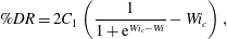 $$\begin{eqnarray}\%DR=2C_{1}\left(\frac{1}{1+\text{e}^{Wi_{c}-Wi}}-Wi_{c}\right),\end{eqnarray}$$
where $C_{1}=64$
is the approximate limiting value of
$C_{1}=64$
is the approximate limiting value of $\%DR$
as
$\%DR$
as $Wi\rightarrow \infty$
and
$Wi\rightarrow \infty$
and $Wi_{c}$
is the critical Weissenberg number for the onset of drag reduction (set to be
$Wi_{c}$
is the critical Weissenberg number for the onset of drag reduction (set to be $Wi_{c}=0.5$
). Hence, we are able to relate the degree of drag reduction to a single measurable extensional rheological property of the polymer solutions independent of flow geometry, concentration, degradation and other experimental variables. The onset of
$Wi_{c}=0.5$
). Hence, we are able to relate the degree of drag reduction to a single measurable extensional rheological property of the polymer solutions independent of flow geometry, concentration, degradation and other experimental variables. The onset of $\%DR$
can be observed to take place at
$\%DR$
can be observed to take place at $Wi\approx 0.5$
, which, although in agreement with the theory of Lumley (Reference Lumley1973), i.e. potentially related to the so-called ‘coil-stretch’ transition, may just be fortuitous because
$Wi\approx 0.5$
, which, although in agreement with the theory of Lumley (Reference Lumley1973), i.e. potentially related to the so-called ‘coil-stretch’ transition, may just be fortuitous because $Wi$
here is based on the average wall shear rate rather than the fluctuating strain rates or the largest Lyapunov exponent (Stone & Graham Reference Stone and Graham2003). MDR is attained at
$Wi$
here is based on the average wall shear rate rather than the fluctuating strain rates or the largest Lyapunov exponent (Stone & Graham Reference Stone and Graham2003). MDR is attained at $Wi\gtrsim 5$
, for which
$Wi\gtrsim 5$
, for which $\%DR$
becomes independent of
$\%DR$
becomes independent of $Wi$
. We note a strong qualitative agreement between the universal form of our experimental data and results from direct numerical simulations (DNS) obtained from various models shown in Housiadas & Beris (Reference Housiadas and Beris2013): however, the DNS data require an additional fitting parameter (‘LDR’), which represents the asymptotic limit of large Weissenberg numbers and is not known a priori. In contrast, equation (5.1) enables the degree of drag reduction at a given flow rate in a given geometry to be estimated (using an iterative procedure) solely if the polymer shear rheology and relaxation time are known.
$Wi$
. We note a strong qualitative agreement between the universal form of our experimental data and results from direct numerical simulations (DNS) obtained from various models shown in Housiadas & Beris (Reference Housiadas and Beris2013): however, the DNS data require an additional fitting parameter (‘LDR’), which represents the asymptotic limit of large Weissenberg numbers and is not known a priori. In contrast, equation (5.1) enables the degree of drag reduction at a given flow rate in a given geometry to be estimated (using an iterative procedure) solely if the polymer shear rheology and relaxation time are known.

Figure 5. (a) Combined $f$
–
$f$
– $Re$
data for cylindrical pipe, rectangular channel and square duct (symbols and colours as in figure 4). (b) Variation of
$Re$
data for cylindrical pipe, rectangular channel and square duct (symbols and colours as in figure 4). (b) Variation of $\%DR$
with Weissenberg number. The solid black line represents the new correlation:
$\%DR$
with Weissenberg number. The solid black line represents the new correlation: $\%DR=2C_{1}[1/(1+\text{e}^{Wi_{c}-Wi})-Wi_{c}]$
.
$\%DR=2C_{1}[1/(1+\text{e}^{Wi_{c}-Wi})-Wi_{c}]$
.
In observing a working functional dependence of $\%DR$
on
$\%DR$
on $Wi$
alone, the dependence on the ratio
$Wi$
alone, the dependence on the ratio $\unicode[STIX]{x1D6FD}$
of solvent to total viscosity, on inertia (i.e. Reynolds number) and on other viscometric functions, e.g. first or second normal-stress differences, is neglected. All of the concentrations are quite similar, all being within the semidilute regime, so the effect of
$\unicode[STIX]{x1D6FD}$
of solvent to total viscosity, on inertia (i.e. Reynolds number) and on other viscometric functions, e.g. first or second normal-stress differences, is neglected. All of the concentrations are quite similar, all being within the semidilute regime, so the effect of $\unicode[STIX]{x1D6FD}$
must contribute to the spread of the data around the fit. We note that the variation in the data is larger than the experimental uncertainty associated with the data, which we estimate to be
$\unicode[STIX]{x1D6FD}$
must contribute to the spread of the data around the fit. We note that the variation in the data is larger than the experimental uncertainty associated with the data, which we estimate to be $\pm 3{-}3.5\,\%$
as highlighted by the representative error bars shown in figure 5(b).
$\pm 3{-}3.5\,\%$
as highlighted by the representative error bars shown in figure 5(b).
In the MDR limit it is also known that there remains some weak $Re$
dependence, as
$Re$
dependence, as $\%DR$
scales roughly as
$\%DR$
scales roughly as $Re^{0.1}$
in this limit, and, as we have already discussed, there is significant spread in the literature for data nominally at MDR (Graham Reference Graham2014), as is highlighted by the grey region in figure 5(b). Given the quality of the data collapse illustrated in figure 5(b), both
$Re^{0.1}$
in this limit, and, as we have already discussed, there is significant spread in the literature for data nominally at MDR (Graham Reference Graham2014), as is highlighted by the grey region in figure 5(b). Given the quality of the data collapse illustrated in figure 5(b), both $\unicode[STIX]{x1D6FD}$
and
$\unicode[STIX]{x1D6FD}$
and $Re$
seem to be second-order effects, at least for the concentrations (of the order of
$Re$
seem to be second-order effects, at least for the concentrations (of the order of $c^{\ast }$
) and range of
$c^{\ast }$
) and range of $Re$
(
$Re$
( ${\approx}10^{3}{-}5\times 10^{4}$
) studied for this particular flexible polymer. Although our data, and the correlation proposed in (5.1), suggest that no critical polymer concentration for drag-reduction onset is required (provided the mean wall shear rate is sufficient to make
${\approx}10^{3}{-}5\times 10^{4}$
) studied for this particular flexible polymer. Although our data, and the correlation proposed in (5.1), suggest that no critical polymer concentration for drag-reduction onset is required (provided the mean wall shear rate is sufficient to make $Wi\gtrsim 0.5$
) we stress that the range of
$Wi\gtrsim 0.5$
) we stress that the range of $\unicode[STIX]{x1D6FD}$
probed here (
$\unicode[STIX]{x1D6FD}$
probed here ( ${\approx}0.1$
) means that the polymeric viscosity (and hence polymeric stress) is never negligible. In the limit where the solvent contribution to the stress dominates (i.e.
${\approx}0.1$
) means that the polymeric viscosity (and hence polymeric stress) is never negligible. In the limit where the solvent contribution to the stress dominates (i.e. $\unicode[STIX]{x1D6FD}\rightarrow 1$
), simulations suggest that a critical concentration is required for onset regardless of shear rate (Lee & Akhavan Reference Lee and Akhavan2009).
$\unicode[STIX]{x1D6FD}\rightarrow 1$
), simulations suggest that a critical concentration is required for onset regardless of shear rate (Lee & Akhavan Reference Lee and Akhavan2009).
We note also no dependence on the Trouton ratio $Tr$
(i.e. the ratio of extensional viscosity to shear viscosity), but in our experiment we cannot independently adjust
$Tr$
(i.e. the ratio of extensional viscosity to shear viscosity), but in our experiment we cannot independently adjust $Tr$
and
$Tr$
and $\unicode[STIX]{x1D706}_{c}$
because both are related to the length of the polymer molecule. Finally the data collected in Graham (Reference Graham2014) for different geometries – boundary layer, pipe and channel flow – also exhibit a similar spread, nominally at MDR, suggesting that some of the spread here could also be related to the use of different geometries and the simplistic estimate of the mean wall shear rate. In particular the square duct, and to a lesser extent the channel, exhibits a mean wall shear rate that varies around its periphery, whereas the pipe is axisymmetric and therefore spatially constant.
$\unicode[STIX]{x1D706}_{c}$
because both are related to the length of the polymer molecule. Finally the data collected in Graham (Reference Graham2014) for different geometries – boundary layer, pipe and channel flow – also exhibit a similar spread, nominally at MDR, suggesting that some of the spread here could also be related to the use of different geometries and the simplistic estimate of the mean wall shear rate. In particular the square duct, and to a lesser extent the channel, exhibits a mean wall shear rate that varies around its periphery, whereas the pipe is axisymmetric and therefore spatially constant.
Finally, it is recommended that a similar procedure be applied to other types of flexible polymers to test the universality of the observed correlation between $\%DR$
and
$\%DR$
and $Wi$
. An attempt to obtain data for polyethylene oxide in our rigs was not successful, because the polymer degrades much more quickly, resulting in large variation in rheological properties within each rig at the same pumping times. Unfortunately such inhomogeneity of degradation precluded the same approach as was possible for the polyacrylamides.
$Wi$
. An attempt to obtain data for polyethylene oxide in our rigs was not successful, because the polymer degrades much more quickly, resulting in large variation in rheological properties within each rig at the same pumping times. Unfortunately such inhomogeneity of degradation precluded the same approach as was possible for the polyacrylamides.
6 Conclusion
In this study, turbulent drag reduction with polyacrylamide, a flexible polymer, has been investigated in a cylindrical pipe, a rectangular channel and a square duct. The polymer solutions were subjected to various levels of degradation by recirculating through the experimental rigs, and their shear and extensional rheological properties were closely monitored. Polymer relaxation times were observed to scale roughly as $t^{-0.5}$
. Profiles of streamwise velocity (
$t^{-0.5}$
. Profiles of streamwise velocity ( $U^{+}$
) at various levels of drag reduction indicated a thickening of the buffer layer as observed in previous experimental studies, the buffer layer extending across the entire cross-section at MDR. A plot of
$U^{+}$
) at various levels of drag reduction indicated a thickening of the buffer layer as observed in previous experimental studies, the buffer layer extending across the entire cross-section at MDR. A plot of $\%DR$
against Weissenberg number was found to collapse the data, with the onset of DR occurring at
$\%DR$
against Weissenberg number was found to collapse the data, with the onset of DR occurring at $Wi\approx 0.5$
and MDR at
$Wi\approx 0.5$
and MDR at $Wi\gtrsim 5$
, thus allowing for an a priori quantitative prediction of drag reduction from a knowledge of polymer relaxation time, flow rate and geometric length scale (using either the Newtonian pressure drop combined with rheology data, or the average shear rate as an initial guess to determine
$Wi\gtrsim 5$
, thus allowing for an a priori quantitative prediction of drag reduction from a knowledge of polymer relaxation time, flow rate and geometric length scale (using either the Newtonian pressure drop combined with rheology data, or the average shear rate as an initial guess to determine $Wi$
, combined with an iterative procedure).
$Wi$
, combined with an iterative procedure).
Acknowledgements
R.J.P. would like to thank the Engineering and Physical Sciences Research Council (EPSRC) for the award of a Fellowship under grant EP/M025187/1. We would also like to thank Professor M. Graham for helpful discussions and the anonymous referees for bringing a number of useful references to our attention.


 Open access