1. Introduction

The overwinter regime of soil water and solute movement is an important issue related to the management of fertilization in agricultural fields, the modeling of plant growth in natural ecosystems and the assessment of groundwater quality in cold regions. However, soil water and anion movements during soil freezing and snow cover remain poorly understood compared with those during the plant-growing season because of the lack of field data and the difficulty in analyzing water movements under soil-freezing conditions.

When a freeze penetrates into deep soil layers in early and mid-winter, upward water movement occurs at and below the frozen layer, which implies the upward movement of solutes. In fact, some researchers have described substantial amounts of upward movement of dissolved materials during this period (Reference Campbell, Ferguson and WarderCampbell and others, 1970; Reference Gray and GrangerGray and Granger, 1986; Reference Nishio, Kanamori and FujimotoNishio and others, 1988). In contrast, the hydraulic conductivity of the frozen soil generally decreases markedly when soil freezes (e.g. Reference MillerMiller, 1970), which implies restricted water and solute movements. Reference Lundin and JohnssonLundin and Johnsson (1994) monitored soil electrical conductivity (EC) using time-domain reflectometry (TDR) and concluded that the ions were transported downward with the penetration of the freezing front by the thermally induced regulation of a brine pocket (Reference Miller and HillelMiller, 1980). These results suggest that the upward solute movement might not be so great in some cases. Field observations and analyses of soil water and anion movement are still necessary because of the limited knowledge of anion movements in this stage.

Snowmelt infiltration strongly influences solute movement to the deep soil layer (Reference Savard, Paradis, Somers, Liao and Van BochoveSavard and others, 2007). However, a thick frozen layer sometimes impedes snowmelt infiltration (e.g. Reference Gray, Toth, Zhao, Pomeroy and GrangerGray and others, 2001; Reference Stähli and AndersonStähli, 2005; Reference Iwata, Gliéski, Horabik and LipiecIwata, 2011), resulting in smaller fluxes of water and solutes in the soil during the snowmelt period. Previous researchers have revealed that frozen soil sometimes impedes snowmelt infiltration, increases the runoff and influences nutrient cycles (e.g. Reference Srinivasan, Bryant, Callahan and WeldSrinivasan and others, 2006). However, the mechanism of solute movement in frozen soil during the snowmelt period is not fully understood.

To elucidate the relations among snow cover, soil frost and soil water movement, field observations were conducted during November 2005–April 2006 in the central part of the Tokachi region, which is located in the northernmost island of Japan and is a major area of crop production. In this region, frost depth has been decreasing markedly over the past 20 years because of an earlier onset of thick snow cover insulating the ground (Reference HirotaHirota and others, 2006). For example, the annual maximum soil frost depth was <0.2 m in the most recent 10 years, although it had been >0.4 m in the prior period. To examine the change in soil water movement in winter during the most recent 20 years, two experimental plots were prepared in an agricultural field (see Section 2 for location). Snow in one plot (treated plot) was removed in early winter to deepen the soil frost depth. Snow in the other plot (control plot) was kept in a natural condition. Analyzing the data of snow, soil temperature, soil water content and soil water flux, Reference Iwata, Hayashi, Suzuki, Hirota and HasegawaIwata and others (2010) revealed that the deep penetration of the freezing front resulting from the snow removal treatment strongly influenced soil water movement during the winter and spring snowmelt periods.

The large difference in soil water movement, which was induced by the difference in soil frost depth between the treated and control plots, suggests a difference in solute movement. As described in this paper, we first show the vertical distribution of nitrate content in the soil during the experiment. Then we use the Simultaneous Heat and Water (SHAW) model (Reference Flerchinger and PiersonFlerchinger and Pierson, 1991; Reference FlerchingerFlerchinger, 2000) to simulate the thickness of snow cover, soil frost depth, soil water movement and nitrate movement in the soil. The results are compared with the measured values. The objectives of this research are to ascertain the soil anion transport mechanisms and to test the performance of the SHAW model in simulating the soil thermal regime, soil water movement and nitrate movement in frozen soil.

2. Materials and Methods

This study was conducted in an experimental field operated by the Hokkaido Agricultural Research Center (42°53’N/143°05’E), located in Memuro, Hokkaido, Japan. The 1981–2010 mean annual precipitation and mean annual air temperature at the Memuro meteorological station, located 2.5 km west of the experimental site, were 957mm and 6.1°C, respectively (Japan Meteorological Agency). The site is covered by a volcanic ash soil (classified as Andosols based on the world reference base (WRB) for soil resources; International Union of Soil Sciences Working Group WRB, 2006), which is a common soil type in Japan. The site has very little topographic relief (<1% slope). The soil is underlain by a gravel layer at 1 m and the water table is generally located ∼8 m below the ground surface in this region (Reference OkaOka, 2000). The soil was well aggregated. No visible cracks were observed throughout the soil profile when it was surveyed before the experiment. Soil textures of the soil layer were silt loam to clay and the total carbon content of the surface soil layer was 36.8 g C kg⁻¹. Details of the location, layout and physical properties of the study plot were described by Reference Iwata, Hayashi, Suzuki, Hirota and HasegawaIwata and others (2010). For details of the chemical properties, see Reference Yanai, Hirota, Iwata, Nemoto, Nagata and KogaYanai and others (2011).

Two square plots (5 m × 5 m) were placed with a separation distance of 2.5 m. The study was conducted during the period 1 November 2005 to 2 May 2006. Before the site installation, oats were planted in the summer of 2005 and harvested in September. After harvest, the soil was plowed to 0.15 m depth and mixed with plant residues. There was no vegetation on the ground during the study period. Snow cover was removed several times between 19 December 2005 and 13 January 2006 at the treated plot. Snow was placed artificially on this plot after the frost depth reached 0.4 m, to avoid further penetration of the frozen layer.

Liquid soil water contents were monitored using a time-domain reflectometry system (TDR100; Campbell Scientific Inc.) with a CS605 probe at a depth of every 0.1 m from 0.05 to 1.05 m. The relations between the soil dielectric constant and volumetric water content were determined in the laboratory using repacked soil columns. Copper-constantan thermocouples were installed in the treated plot from the surface down to 1 m at depths of 0.00, 0.02, 0.05, 0.10, 0.15, 0.20, 0.25, 0.30 and 0.35 m and every 0.1 m between 0.4 and 1.0 m. The soil temperature was also monitored at the control plot at the same depths as in the treated plot except for 0.25 and 0.35 m. Soil was considered frozen when the temperature was <0°C. Soil matric potential at depths of 0.9 and 1.0 m was measured using tensiometers that had been designed specifically for monitoring the potential of unfrozen soil below the frozen layer (Reference Iwata and HirotaIwata and Hirota, 2005a,Reference Iwata and Hirotab). The data were used to calculate the soil water flux between them using Darcy’s law (Reference Iwata, Hayashi, Suzuki, Hirota and HasegawaIwata and others, 2010). Soil water flux at 0.4 m depth, which was almost equal to the maximum frost depth at the treated plot, was calculated from the soil water flux and soil water contents monitored between 0.4 and 1.0 m depths using the water-balance method (for detailed calculation, see Reference Iwata, Hayashi, Suzuki, Hirota and HasegawaIwata and others, 2010).

Precipitation, air temperature, solar radiation and wind speed were measured at an observation site located ∼100 m east of the site. Precipitation was measured using an overflow type tipping-bucket rain gage (B071-20; Yokogawa Analytical Systems Inc.) with a heated water reservoir and a windshield (RT-4; Yokogawa Analytical Systems Inc.). The air temperature was monitored at 1.5 m above the ground using a platinum resistance sensor (C-HPT-5-JM; Climatec Inc.). Solar radiation was monitored using a pyranometer (CM-21; Kipp &amp; Zonen). Wind speed was monitored at 10 m from the ground using an anemometer (Model 05103; R.M. Young Co.). The snow thickness and snow water equivalent (SWE) were measured manually twice a week at the control and treated plots. SWE was measured using a 50 mm internal diameter aluminum snow survey tube.

Vertical distributions of nitrate nitrogen to 1 m depth were determined for triplicate soil cores that were sampled using a soil sampling system (PC-liner, DIK-162B; Daiki Rika Co. Ltd) consisting of a cylindrical soil sampler of 50 mm inner diameter, an engine-drive hammer to install the sampler and a mechanical jack to pull back the sampler. The soil sampling was conducted before (15 November 2005), during (25 January 2006) and after (2 May 2006) soil freezing. The 1 m soil samples were cut into 70–100mm sections and transferred to the laboratory. Samples were put into a plastic bottle with distilled water and the bottle was shaken for 1 hour. Liquids in the suspension were filtered and the nitrate content of the liquid was measured using ion-exchange chromatography (IA-100; TOA Corp.).

The SHAW model was used to simulate the snow-cover thickness, soil frost depth, soil water movement and nitrate movement. This model calculates the snow-cover thickness from precipitation, air temperature, solar radiation and wind speed (Reference Flerchinger, Baker and SpaansFlerchinger and others, 1996). To determine the initial condition of the new snow layer, we assumed snow densities of 80 and 200 kgm⁻³, respectively, in cases with air temperature below and above 0°C. Thermal processes in soil are calculated from the upper and lower conditions of the soil layer and the equations to describe the transportation of heat and water. The model determines the upper boundary condition from the energy-balance equation. We used the soil temperature measured at 1.0 m depth as the lower boundary condition. Soil to 1.0m depth was divided into 11 layers, and boundaries of each layer were regarded as the node for the calculation (Fig. 1). Soil properties of each node were regarded as equal to those of the soil layer that includes the node. The SHAW model calculates the soil thermal conductivity using the de Vries (1963) equation. Dry bulk density was determined from the cylindrical soil samples of 50 mm height and 51 mm diameter, which were sampled from each soil layer. Saturated hydraulic conductivity and the water characteristic curve were also ascertained from the soil samples. The hydraulic conductivity was measured using the constant-head core method (Reference Dane and ToppDane and Topp, 2002). The relations between water content and matric potential were measured using the hanging water column method in wet conditions (>–0.3 m of matric potential head) and the pressure cell method in dry conditions (<–0.3 m of matric potential head) (Reference Dane and ToppDane and Topp, 2002). The soil water characteristic curve at each soil layer was obtained using the equation developed by Reference Brooks and CoreyBrooks and Corey (1966). Fitting parameters to this equation were determined to minimize the root-mean-square error (RMSE) between measured and calculated soil water contents at the same matric potential. The fitting parameter of the curve and the saturated hydraulic conductivity were used to estimate the unsaturated conductivity using a simple equation developed by Reference CampbellCampbell (1974). Solute transfer was calculated using an equation incorporating molecular diffusion, convection and hydrodynamic dispersion in the liquid phase of the soil matrix pore (Reference FlerchingerFlerchinger, 2000). Some volcanic ash soils adsorb anions and delay solute movement (Reference Katou, Clothier and GreenKatou and others, 1996). Reference Tamura, Nakahara, Tanaka, Kato and HasegawaTamura and others (2011) showed that marked anion adsorption occurs in the 1C layer, which was located immediately below the surface layer in our experimental field. To reflect the delay in nitrate movement, we used 0.76 for the equilibrium partition coefficient of the solute and liquid and solid matrix of this layer, which was determined by laboratory experiment (Reference Tamura, Nakahara, Tanaka, Kato and HasegawaTamura and others, 2011). Although nitrate in the soil might increase and decrease because of the activity of microbes, this phenomenon was not considered in the simulation. The measured profiles of soil water content, soil temperature and nitrate content were used as the initial conditions. To simulate snow removal, we stopped the model calculation when the snow-cover treatment (removal and replacement) was conducted, and resumed the calculation using the initial profiles of soil temperature and water content at the end of the previous calculation.

Fig. 1. Soil profile, depth of node for the calculation using the SHAW model, saturated hydraulic conductivity (ks) and dry bulk density (p_d) at each soil layer. Values outside and inside the parentheses of soil profiles denote the boundaries of the control and treated plots, respectively.

3. Results

3.1. Snow-cover thickness and soil frost depth

Time series of snow-cover thickness and soil frost depth with daily mean air temperature and precipitation are shown in Figure 2. Soil started freezing from the surface in late November, when the daily average air temperature fell and remained below 0°C. We designate the period during which the significant penetration of the freezing front was observed as the freezing period (period I in Fig. 2). Significant penetration of the freezing front stopped when the snow-cover thickness was >0.3m through snowfall or artificial loading of snow. We designate the period from the end of the freezing period to the onset of snowmelt as the snow-covered period (period II in Fig. 2). Although continuous snowmelt started in early March, a substantial amount of rain fell on 25 February 2006 and the frozen layer started to thaw (Reference Iwata, Hayashi, Suzuki, Hirota and HasegawaIwata and others, 2010). The snow cover disappeared on 22 March 2006. We designate the period between 25 February and 22 March 2006 as the first snowmelt period (period III in Fig. 2). A large amount of snow fell on 29 March 2006, melting completely by 18 April 2006. We designate this period as the second snowmelt period (period IV in Fig. 2).

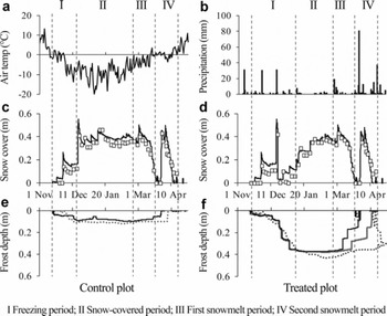
Fig. 2. Time series of (a) air temperature, (b) precipitation, (c, d) snow-cover thickness and (e, f) soil frost depth during November 2005–April 2006. Air temperature and frost depth are daily averages. Precipitation is the amount. Solid black lines of snow-cover thickness and frost depth are values estimated using the SHAW model. Open squares of snow-cover thickness and dotted lines of soil frost depth are measured values. Solid gray line in (f) shows the lower boundary of the frozen layer simulated to be the initial soil water content higher than the observed value (see Section 4 for details).

The RMSEs in the control and treated plots between simulated snow-cover thickness using the SHAW model and measured values throughout the observation period were 0.046 and 0.048 m, respectively, suggesting reasonable agreement with the measured values (Fig. 2c and d). The RMSEs at the control and treated plots between simulated and measured soil frost depths were 0.028 and 0.037 m, respectively, during the freezing and the snow-covered periods (periods I and II in Fig. 2). These were close to 0.035 m, which was the RMSE between the frost depths measured by the frost tube and determined from the soil sample (Reference Iwata, Gliéski, Horabik and LipiecIwata and others, 2011), suggesting that the SHAW model can simulate soil frost depth reasonably before the onset of snowmelt. In contrast to these periods, the frozen soil thawed from the bottom of the frozen layer earlier than the measured values during the snowmelt periods (periods III and IV in Fig. 2). The difference between measured and simulated soil frost depths was substantial, especially in the treated plot.

3.2. Soil water movement before the onset of snowmelt

Cumulative values of upward soil water flux at 0.4 m depth, which were calculated from the field data (Σq_0.4__m), were 18 and 41 mm, respectively, in the control and treated plots before the onset of snowmelt (Fig. 3). In the control plot, Σq_0.4_m was only 0.8mm during the freezing period, suggesting that most of the upward soil water movement occurred during the snow-covered period (Fig. 3a). In contrast, Σ_q0_.4_m during the freezing period was three times larger than that during the snow-covered period in the treated plot (Fig. 3b).

Fig. 3. Cumulative upward soil water fluxes between depths before the onset of snowmelt in (a) the control plot and (b) the treated plot, as calculated using the SHAW model. Cumulative fluxes at 0.4m depth, as calculated from the measured data, are also shown. Black bars show the cumulative values in the freezing period; gray bars are those in the snow-covered period.

The cumulative soil water fluxes simulated by the SHAW model (Σ _{q SHAW}) were also positive to 0.4 m depth during the freezing period in both plots (Fig. 3). However, Σ _{q SHAW} between 0.4 and 0.5 m depth was 0 mm during the freezing and snow-covered periods in both plots, suggesting no water supply from the deep layer to above 0.4 m depth during the cold winter in the simulation. Σ_q0.4_m during the freezing and snow-covered periods was comparable with the average Σ _q SHAW at 0.2–0.3 m and 0.3–0.4 m in the control plot (Fig. 3a). Total Σq_{0.4_m} was larger than any Σq _SHAW value in the treated plot (Fig. 3b).

The measured values of Σ _{q SHAW} during the soil-freezing period were much larger than those during the snow-covered period at all depths in the control plot, which was contrary to the Σ_q0.4__m (Fig. 3a). Σ _{q SH}AW during the snow-covered period was 0mm at all depths in the treated plot, resulting in the smaller total Σq _SHAW than that in the control plot (Fig. 3). This result was also contrary to the relation found for the total Σ_q0.4 _m between the treated and control plots.

3.3. Soil water movement during the snowmelt period

Cumulative downward soil water fluxes during the first and second snowmelt periods are shown in Figure 4. In contrast to Σ _{q SHAW} during the freezing and snow-covered periods, no significant difference was found among values of Σ _{q SHAW} at different depths in both plots. The sum of Σ_{q0.4_m} during the first and second snowmelt periods in the control plot was greater than that in the treated plot resulting from the large Σq_0.4__m during the first snowmelt period in the control plot. In contrast, Σq _SHAW in the treated plot was almost identical to those in the control plot. Σ _{q SHAW} values were very small or 0 mm at all depths during the first snowmelt period in both plots, which contrasted with Σ_{q0.4_m}, especially in the control plot. Σ _{q SHAW} values were comparable with Σq _{0.4_m} during the second snowmelt period in both plots.

Fig. 4. Cumulative downward soil water fluxes between each depth in the snowmelt period in (a) the control plot and (b) the treated plot, as calculated using the SHAW model. Cumulative fluxes at 0.4m depth, as calculated from the measured data, are also shown. First and second cumulative fluxes were measured during 25 February–22 March 2006 and 29 March–17 April 2006, respectively.

3.4. Profile of nitrate content

The nitrate content profiles are presented in Figure 5. The peak in nitrate content was located between 0.2 and 0.3 m depth before the soil was frozen. The profile shapes on 25 January 2006, when soil frost depths were 0.11 and 0.41 m, respectively, at the control and the treated plots (Fig. 2), were not different from those of 15 November 2005 in either plot. However, simulated profiles using the SHAW model suggest that a substantial amount of nitrate moved upward in both plots until 25 January 2006. After the snowmelt period, the measured peak of nitrate content in the control plot was deeper than that in the treated plot. In contrast, the simulated profiles of nitrate content in the control and treated plots (Fig. 5e and f) were almost identical.

Fig. 5. Profiles of nitrate content measured by soil sampling (solid circles) and estimated using the SHAW model (solid lines). Error bars show standard errors of triplicate soil samples. Soil samples before freezing (a, b) were sampled on 15 November 2005. Those from mid-winter (c, d) and after thawing (e, f) were taken on 25 January and 2 May 2006, respectively. The estimated values in mid-winter and after thawing represent results obtained on 25 January and 30 April 2006, respectively. The dotted line in (e) is the profile simulated under the assumption that the frozen soil layer melted completely at the beginning of the first snowmelt period (see Section 4 for details).

4. Discussion

The SHAW model simulated the snow-cover thickness reasonably well (Fig. 2). The snow-cover thickness influences the thermal dynamics under the ground (e.g. Reference Thorud and DuncanThorud and Duncan, 1972; Reference Decker, Wang, Waite and ScherbatskoyDecker and others, 2003; Reference Iwata, Hayashi and HirotaIwata and others, 2008). Therefore, this model can simulate the soil frost depth. In fact, the soil frost depth was simulated reasonably well using this model during the freezing and the snow-covered periods in each plot (Fig. 2). However, the frozen soil thawed earlier in both plots during the snowmelt period in the simulation compared with the observed data.

4.2. Upward transportation of nitrate before the onset of snowmelt

The simulated profile of nitrate content on 25 January 2006 suggests that a substantial amount of nitrate nitrogen moved to the soil surface in both plots (Fig. 5), which is consistent with results of previous studies showing that the soil water moves upward with the penetration of the freezing front (e.g. Reference Gray and GrangerGray and Granger, 1986; Reference Nishio, Kanamori and FujimotoNishio and others, 1988). However, the shapes of the measured profile of nitrate content on 15 November 2005 and 25 January 2006 did not change significantly.

Although the amount of nitrate content in the soil layer to 1.0 m depth on 15 November 2005 was smaller than that on 25 January 2006, especially in the control plot, no significant downward flux was observed between 15 November 2005 and 25 January 2006 (Fig. 3). Therefore, significant leaching of nitrate to a depth below 1.0 m might not have occurred during this period.

Immobilization, mainly caused by microbe activities, might also decrease nitrates in the soil. Field experiments conducted in pastureland revealed that substantial amounts of nitrate are immobilized in a short period at the surface soil layer (Reference Williams and HaynesWilliams and Haynes, 1994; Reference Saarijärvi and VirkajärviSaarijärvi and Virkajärvi, 2009). However, Reference Nishio and AraoNishio and Arao (2002) took soil samples from crop fields and incubated them at 25°C and reported that only 2.8% of dressed nitrate in the soil sample of Andosols, the same soil type as in the present study, immobilized 90 days after the start of the experiment. Therefore, a decrease in nitrate up to 25 January 2006 might not be attributable to nitrate immobilization.

Denitrification presents another reason for a reduction in nitrate content. Previous studies suggest vigorous N²O production in soil even when the frozen soil layer has formed (Reference Maljanen, Virkajärvi, Hytonen, Öquist, Sparrman and MartikainenMaljanen and others, 2009; Reference Virkajärvi, Maljanen, Saarijärvi, Haapala and MartikainenVirkajärvi and others, 2010). However, Reference Yanai, Hirota, Iwata, Nemoto, Nagata and KogaYanai and others (2011) demonstrated that the soil gas O² concentration did not decrease before the onset of snowmelt and that the concentration of N²O in the soil gas increased from the end of winter in our study field. Therefore, denitrification might not be a factor in explaining the decrease in nitrate content between 15 November 2005 and 25 January 2006.

It is more likely that the differences in nitrate content between these periods are induced by the variation in nitrate content in each plot, which means that it is difficult to compare the amount of nitrate content measured in different periods. However, the small standard errors on 25 January 2006 suggest that the vertical distribution of the nitrate contents of triplicated soil cores were similar in each plot in this period. Therefore the immobile peak in nitrate content from 15 November 2005 to 25 January 2006 (Fig. 5) suggests that no significant nitrate movement occurred during this period.

Most of the simulated upward soil water flux occurred during the early stage of the soil-freezing period, when the simulated soil frost depth was <0.05 m (Fig. 6). In contrast, the measured cumulative water flux at 0.4 m depth was very small during the freezing period in the control plot (Fig. 3). The cumulative soil water flux at 0.2 m depth was also calculated as 8mm in this period using field measurement data in the control plot, suggesting that significant upward soil water movement did not occur at 0.2 m depth, where the peak of the nitrate content was located, during the freezing period in the control plot. Improvement of the soil water movement process during soil freezing and the snow-covered periods might be necessary to simulate the nitrate movement in our experimental field reasonably well using the SHAW model.

Fig. 6. Time series of soil frost depth (solid black line) and upward soil water fluxes at depths of 0.05–0.10 m (solid gray line) and 0.1–0.2 m (dashed black line) in the control plot, as calculated using the SHAW model.

Summary and Conclusion

Snow removal treatment increased the maximum soil frost depth to 0.43 m; it was 0.11 m in the control plot. Although upward soil water movement below the frozen layer was observed during the soil-freezing and snow-covered periods, especially in the treated plot, significant movement of nitrate nitrogen was not observed during 15 November 2005 to 25 January 2006, when a firm frozen layer formed. The snow was put back on the treated plot when the soil frost depth was 0.4m, resulting in an almost identical amount of snow between the two plots at the beginning of the snowmelt period. Nevertheless, the peak in nitrate content was shallower in the treated plot probably because of the smaller amount of snowmelt infiltration at this plot.

It is possible to simulate snow-cover thickness reasonably well through the observation period using the SHAW model, which can also simulate soil frost depth reasonably well before the onset of snowmelt in both treated and control plots. However, the simulated thawing of soil was earlier than the observed data, probably because of underestimation of the ice content in the frozen layer and overestimation of the thermal conductivity below the frozen layer. The ice content might increase by setting the initial soil water content higher than the observed value or by simulating the amount of water supply from the deep soil layer to the frozen layer reasonably well, which delays the thawing of the frozen layer in the simulation.

Although significant nitrate movement was not observed during the soil-freezing period, a large amount of nitrate movement was simulated in early winter using the SHAW model. In the simulation, a substantial amount of water moved upward in the early freezing period, resulting in the large amount of nitrate movement to the soil surface. In contrast, the observed upward soil water flux below the frozen layer was not significant in early winter. Simulation of nitrate movement is expected to be improved by increasing the accuracy of estimating the soil water movement in early winter.

We were unable to simulate the infiltration process well during the first snowmelt period because of the low permeability of the frozen layer in the simulation. The cumulative downward water flux during the snowmelt period was approximately half of the cumulative flux calculated from the field data at the control plot, resulting in the shallower peak of nitrate content after the snowmelt period in this plot. The simulated profile of nitrate content, with the soil temperature above 0°C at the beginning of the first snowmelt period, was closer to the measured profile in the control plot because the cumulative downward water flux in the first snowmelt period was increased by this treatment. In the treated plot, the difference between simulated and measured peak of nitrate content was much closer than in the control plot. However, this peak was induced by earlier thawing of the frozen layer in the simulation than in the measurement at this plot.

These results suggest that accurate estimation of the soil water movement is necessary to simulate the soil melting process and solute movement precisely. To improve the SHAW model, additional research must be undertaken at a location which has similar soil and meteorological conditions to those of the study site.