Quantitative genetic analysis primarily concerns the analysis of inter-individual variation. A random sample of genetically informative cases (e.g., twin pairs) is drawn from a population of interest. Subsequently, the phenotypic variation between these sampled cases is used to infer the true state of affairs in the population (generalization from sample to population). But this use of inter-individual variation is based on the assumption that the population is homogeneous, in particular that each case in the population obeys the same parametric model. Most quantitative genetic modeling makes this assumption (but see Purcell, Reference Purcell2002, for a notable exception to this rule). For instance, in the seminal paper on multivariate genetic factor analysis (Martin & Eaves, Reference Martin and Eaves1977), the factor loadings and residual variances (including measurement error variances) in the genetic factor model are assumed to be invariant across cases in the population of interest (or subpopulation of interest, in case there are, for instance, sex differences). In what follows this will be referred to as the homogeneity assumption.
Apart from mixture modeling, where it is assumed that there exists a strictly finite number of homogeneous subpopulations capturing only a limited aspect of heterogeneity, it is not often tested whether the homogeneity assumption holds or is violated. Yet the a priori feasibility of the homogeneity assumption would seem to be questionable for a variety of mathematical, biological, and statistical reasons. In Molenaar et al. (Reference Molenaar, Boomsma and Dolan1993) it is argued that nonlinear epigenesis of neural growth yields inter-individual differences in cortical network architecture that are not due to genetic or environmental influences, but are an inevitable outcome of the self-organizing epigenetic processes concerned (cf. also Kan et al., Reference Kan, Ploeger, Raijmakers, Dolan and van der Maas2010; McLachlan, Reference McLachlan, Chaplain, Singh and McLachlan1999; Molenaar Reference Molenaar2007; Molenaar & Raijmakers, Reference Molenaar and Raijmakers1999). A review of inbreeding studies presented in Molenaar et al. (1993) indicates that the amount of inter-individual variation due to developmental noise (e.g., Jablonka, Reference Jablonka, Gissis and Jablonka2011), can be substantial. It is indeed a common finding in brain imaging studies that neural network structures show large inter-individual variation (e.g., Hillary et al., Reference Hillary, Medaglia, Gates, Molenaar, Slocomb, Peechatka and Good2011; Miller & van Horn, Reference Miller and van Horn2007; Miller et al., Reference Miller, van Horn, Wolford, Handy, Valsangkar-Smyth, Inati and Gazzinga2002; Sporns, Reference Sporns2010; but see van Beijsterveldt et al., Reference van Beijsterveldt, Molenaar, de Geus and Boomsma1998b, for high monozygotic intercorrelation of EEG coherence).
From these brain-imaging results it could be expected that the observed heterogeneous cortical organization gives rise to structural variation between subjects in cognitive information processing, and thus poor fit of models that assume homogeneity. Yet it is commonly found that models having invariant parameters yield good fits to the data. This, however, may be explained by the findings from a series of simulation studies (Molenaar, Reference Molenaar2007) that factor analysis of inter-individual variation is insensitive to the presence of widespread variation. In this report, data were simulated by means of subject-specific factor models (each subject having unique factor loadings and measurement error variances). Yet, despite this maximum violation of the homogeneity assumption underlying analysis of inter-individual variation, standard factor analysis of this simulated data, made with the assumption of homogeneity, yielded excellently fitting models. This result was obtained for cross-sectional, longitudinal, and genetic factor models (reviewed in Molenaar, Reference Molenaar2007). Moreover, the insensitivity of factor analysis of inter-individual variation to violations of the homogeneity assumption was proved analytically in Kelderman & Molenaar (Reference Kelderman and Molenaar2007).
The prime method of identifying violations of the homogeneity assumption is analysis of intra-individual variation (i.e., replicated time-series analysis; Hamaker et al., Reference Hamaker, Dolan and Molenaar2005). In what follows, whether the two members of a single dizygotic (DZ) twin pair obey the same genetic factor model will be tested by means of time-series analysis of intra-individual variation. The label ‘iFACE’ (Molenaar, Reference Molenaar, Hood, Halpern, Greenberg and Lerner2010; Nesselroade & Molenaar, Reference Nesselroade and Molenaar2010) is a combination of the idiographic filter (IF) introduced in Nesselroade et al. (Reference Nesselroade, Gerstorf, Hardy and Ram2007), and the ACE acronym for additive, common, and specific environmental factors. The IF allows factor loadings for different subjects to be subject-specific, while defining equivalence of factors across subjects by constraining factor intercorrelations to be invariant across subjects. iFACE (defined below) is a generalization of the longitudinal genetic factor model (LGFM), allowing for subject-specific factor loadings and residual variances. The subject-specificity of model parameters in the iFACE is unrestricted, in contrast to approaches in which such subject-specificity depends upon measured moderators (Purcell, Reference Purcell2002). The iFACE enables a direct test of the homogeneity assumption. In the empirical illustration presented below, it will be fitted to multi-lead event-related brain potential data.
The Model
The iFACE model used to estimate subject-specific heritabilities from a multivariate time series obtained with a single DZ twin pair is a straightforward generalization of the standard LGFM for the analysis of inter-individual variation. That is, the overall structure of iFACE and LGFM is the same. In particular, the additive, common and specific environmental factors obtain their identity/interpretation in the same way, namely through their respective patterns of correlations among the two members of a DZ twin pair. The main difference between the iFACE and the LGFM is the following. In the LGFM the matrix of factor loadings and the covariance matrix of residuals is (a) invariant across DZ twin pairs, and (b) invariant across the members of each twin pair (see Neale et al., Reference Neale, Roysamb and Jacobson2006, for moderation of these model parameters). In contrast, in the iFACE, the matrix of factor loadings is subject-specific in that it is not constrained to be equal for the two members of the given single DZ twin pair. Because the phenotypic data of only a single DZ twin pair are analyzed, the homogeneity assumption across twin pairs also does not apply. The iFACE model combines the idiographic filter (IF) introduced in Nesselroade et al. (Reference Nesselroade, Gerstorf, Hardy and Ram2007), and the ACE model that includes additive, common, and specific environmental (latent) factors. The identity/interpretation of factors in the IF is not based on the pattern of factor loadings (as is the general approach in factor analysis), but instead is based on the pattern of intercorrelations among factors. Hence, in applications of the IF, the matrix of factor loadings is not constrained to be invariant across cases, as it is in the iFACE.
The formal specification of iFACE for a p-variate vector of phenotypic values measured at T equidistant time points is as follows. Let y(t)jm be the m-th phenotypic value (m = 1,. . .,p) obtained for the j-th member (j = 1,2) at time t (t = 1,. . .,T); let A(t)j, C(t)j and E(t)j denote, respectively, the additive (A), common environmental (C), and specific environmental (E), common factor for the j-th member at time t; and let e(t)jm be the m-th residual for the j-th member at time t. It is assumed that residuals obey the conditional independence assumption in that, for all times t = 1,. . .,T, e(t)jm and e(t)jn are uncorrelated among the two members for all m,n = 1,. . .,p, and are uncorrelated within each member for m ≠ n. Note that this allows for the possibility that for each member j ∈ {1,2} each univariate residual process e(t)jm, m = 1,. . .,p, has arbitrary sequential dependencies.
It is assumed that all time series in the iFACE model (i.e., y(t)jm, A(t)j, C(t)j, E(t)j, e(t)jm) are weakly stationary. Weak stationarity of a univariate time series implies that its mean level is a constant (which will be fixed at zero, hence each time series in the iFACE model is assumed to be centered), and that its covariance function (the standard measure of sequential dependencies), depends only upon the relative distance (lag) between time points. In particular, the covariance function of e(t)jm, the univariate residual process associated with the m-th phenotype of the j-th member, is defined as ce(u)jm = cov[e(t)jm, e(t-u)jm], where u denotes the lag (relative time difference). In general ce(u)jm will be nonzero for u = 0, ±1, . . .
With these definitions in place, the iFACE can be defined as:

Note that the additive genetic (αjm), common environmental (δjm) and specific environmental (ϕjm) factor loadings are subject-specific in that they depend upon j and hence are allowed to differ between the two members of the DZ twin pair. The final three equations describe the time evolution of, respectively, the additive genetic, common environmental, and specific environmental, factor scores. This time evolution is modeled as a first-order autoregression, where the autoregressive coefficients (βj, γj, νj) again are allowed to be subject-specific.
The so-called innovations processes ζ(t)j, ξ(t)j and χ(t)j lack any sequential dependencies. Moreover, they are mutually uncorrelated: cov[ζ(t)j, ξ(t)j] = cov[ζ(t)j, χ(t)j] = cov[χ(t)j, ξ(t)j] = 0. The innovation processes associated with the common environmental factor score evolution of twin 1 and 2 are the same: cov[ξ(t)1, ξ(t)2] = 1. Consequently, γ1 = γ2. The innovation processes associated with the specific environmental factor score evolution of twin 1 and 2 are uncorrelated: cov[χ(t)1, χ(t)2] = 0.
The covariance function of the innovations processes associated with the additive genetic factor scores of twin 1 and 2 is estimated: cov[ζ(t)1, ζ(t)2] = σζ. This is because, for a given DZ twin pair, the additive genetic correlation is unknown; it is known only that the average of this correlation across all DZ twin pairs in the population is .5 (Visscher et al., Reference Visscher, Macgregor, Benyamin, Zhu, Gordon, Medland, Hill, Hottenga, Willemsen, Boomsma, Liu, Deng, Montgomery and Martin2007).
The description of the evolution of the additive genetic, common, and specific environmental factor scores by first-order autoregressions can be replaced by autoregressions of arbitrary order. The latter, more general, version of iFACE has been subjected to an alpha-numerical test of parameter identifiability. That is, the dimension of the null space of the first-order derivatives of the model with respect to the free parameters was determined (cf. Bekker et al., Reference Bekker, Merckens and Wansbeek1994), and found to be zero. The test is based on the block-Toeplitz covariance matrix associated with iFACE (see explanation in next section). The Maple session concerned is documented as appendix S1. Hence the general version of iFACE, and therefore also the more specific version described above, is structurally identifiable. In particular, the covariance function of the innovations process associated with the additive genetic factor series of twin 1 and 2 (i.e., β1, β2 and σζ) is structurally identifiable.
An Illustrative Application to Real Data
The iFACE model requires longitudinal datasets with many repeated observations measured in DZ twin pairs. Therefore, we chose to analyze data from electrophysiological time series.
The participants were selected from a large dataset of EEG recordings in twins and additional siblings. The participant description and experimental setup are more fully described elsewhere (van Beijsterveldt et al., Reference van Beijsterveldt, Molenaar, de Geus and Boomsma1998a; Smit et al., Reference Smit, Posthuma, Boomsma and de Geus2007). The final set consisted of two complete DZ twin pairs who were randomly selected from the subset of participants with high quality data (all electrodes provided good signal), with ages between 20 and 30. These subjects were one male DZ twin pair age 27, and one female DZ twin pair age 29. The experiment was approved by the Medical Ethics Committee of the VU Medical Center. All subjects gave written informed consent.
EEG was measured during a so-called oddball task, in which an infrequent (20%) target stimulus is presented amongst frequent nontarget stimuli (80%). The stimuli were white-on-black line drawings of cats and dogs. The dog stimuli were shown frequently (100/125) and were the nontargets. The cat stimuli were shown only infrequently (25/125) and were the targets. Dog and cat stimuli were presented in an unpredictable order, and trial duration varied randomly from 1500 to 2000 ms. Stimulus duration was 100 ms. Subjects were instructed to silently count the number of targets (cats) shown on the computer screen positioned 80 cm in front of them.
The EEG was recorded with tin electrodes in an ElectroCap connected to a Nihon Kohden PV-441A polygraph with time constant 5 s (corresponding to a 0.03 Hz high-pass filter), and lowpass of 35 Hz, digitized at 250 Hz using an in-house built 12-bit A/D converter board, and stored for offline analysis. Leads were Fp1, Fp2, F7, F3, F4, F8, C3, C4, T5, P3, P4, T6, O1, O2, and bipolar horizontal and vertical EOG derivations. Electrode impedances were kept below 5 kΩ. Following the recommendation by Pivik et al. (1991), tin earlobe electrodes (A1, A2) were fed to separate high-impedance amplifiers, after which the electrically linked output signals served as reference to the EEG signals. Sine waves of 100 μV were used for calibration of the amplification/AD conversion before measurement of each subject.
Standard data cleaning procedures were maintained, and eye-blink artifacts were removed using Independent Components Analysis (Jung et al., Reference Jung, Makeig, Humphries, Lee, McKeown, Iragui and Sejnowski2000). The total multi-lead EEG data set of the twin pair consists of 19 replications of the brain response to the rare stimulus measured during 1024 ms post-stimulus, amounting to 256 observations per replication per person. The event-related potential (ERP) brain responses to these rare stimuli at a representative parietal location are shown in Figure 1 for both DZ twin pairs.
FIGURE 1 ERP waves of dizygous twin pair A (top) and dizygous twin pair B (bottom) for representative parietal leads. Grey area indicates standard error based on trial-to-trial variation.
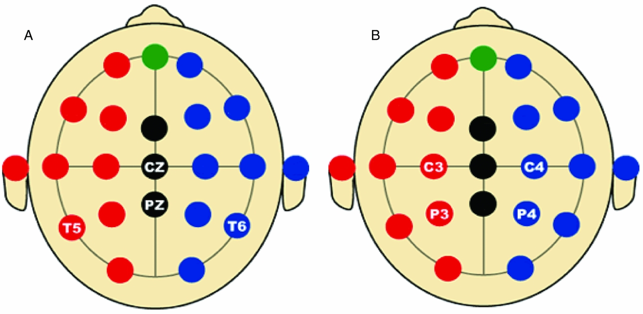
In the first analysis, only the data of the four leads depicted in Figure 2A (Cz, Pz, T5 and T6) are analyzed. Hence p = 4 in the iFACE defined above. These leads correspond to the topography of the main brain response to rare stimuli in an oddball task. A subset of four leads was chosen in order to ease the model fit. Model fits were carried out by means of the block-Toeplitz covariance matrix method described in Molenaar (Reference Molenaar1985). Let Cy(u) denote the (p,p)-dimensional covariance matrix of the p-variate phenotypic series y(t) at lag u, where u ∈ {0, ±1, ±2, . . .} (boldface lowercase and uppercase letters denote, respectively, column vectors and matrices). That is, Cy(u) = cov[y(t), y(t−u)T], where the superscript T denotes transposition. Notice that Cy(−u) = Cy(u)T. For a finite maximum lag U define the (pU+p, pU+p)-dimensional block-Toeplitz covariance matrix Cy associated with y(t) as having Cy(k-m) as its (k,m)-th block, k,m = 0, ±1,. . ., ±U. The block-Toeplitz covariance estimates were calculated for each of the replications. Table 1 presents the results of applying the block-Toeplitz method to simulated data, corroborating its fidelity in that the simple 95% confidence interval around each parameter estimate includes its true value. The iFACE is rewritten as a factor model involving extended patterned parameter matrices, with patterns and dimensions that are conformable with the block-Toeplitz pattern of Cy. Standard SEM software (Jöreskog & Sörbom, Reference Jörekog and Sörbom1992) is used to fit the iFACE to Cy (viz., the average of the block-Toeplitz covariance estimations across replications) by means of the quasi-maximum likelihood method. In the present applications, as well as in the Maple session reported in Appendix S1, U = 1, which is the minimum value necessary to identify the iFACE. The Lisrel source code used in fitting the iFACE to the empirical and simulated data is specified in Appendix S2.

FIGURE 2 Selected electrode locations in the first (A) and second (B) applications of iFACE.
TABLE 1 Results of the Analysis of Simulated Event-Related Potential Data
A set of 10 replications of 4-variate phenotypic time series, each of length 256, have been simulated according to the iFACE model for a single dizygotic twin pair. The true model parameters have values resembling those in Table 2, except that the measurement error series are white noise series having unit variance. To enable direct comparison between true and estimated parameter values, the model was fitted to the average block-Toeplitz covariance matrix pooled across replications. The Lisrel code is presented in appendix S2. Each entry specifies the true value, its estimate and standard error within parentheses. The true additive genetic correlation is σ = .5; its estimate is .56 (.10). The likelihood ratio is 41.52 (df = 97).
Results
The results of fitting the iFACE to the empirical event-related brain potential data of the four leads depicted in Figure 2A are presented in Table 2. In the second analysis, only the data of the four leads depicted in Figure 2B (C3, C4, P3 and P4) are analyzed. These leads also correspond to the topography of the main brain response to rare stimuli in an oddball task. The results are presented in Table 3. In both analyses the autoregressive coefficients in the iFACE are about .9, with standard errors smaller than .11.
TABLE 2 Variance Components Obtained in the First Application of iFACE to Event-Related Potentials of Medial and Lateral-Temporal EEG Leads of a Single Dizygotic Twin Pair
The estimated genetic correlation for the dizygotic twin pair cor[A(t)1, A(t)2] = .40. The phenotypic variance at each EEG electrode location was standardized at 1.0. The final column e(t).m2 gives the contribution of the residual process at each electrode location. The decompositions of the communal part at each electrode location is (1.0 – e(t).m2) and is given in the first three columns as proportions of the communal parts.
TABLE 3 Variance Components Obtained in the Second Application of iFACE to Event-Related Potentials of Central and Parietal EEG Leads of a Single Dizygotic Twin Pair
The estimated genetic correlation for the dizygous twin pair cor[A(t)1, A(t)2] = .37. The phenotypic variance at each EEG electrode location was standardized at 1.0. The final column e(t).m2 gives the contribution of the residual process at each electrode location. The decompositions of the communal part at each electrode location is (1.0 – e(t).m2) and is given in the first three columns as proportions of the communal parts.
The results presented in Tables 2 and 3 were obtained as follows. The final column shows for each twin and each phenotype the proportion of the total phenotypic variance (normalized at 1.0) explained by the residual processes e(t)jm. For instance, for Twin 1, a proportion of .703 of the phenotypic variance at Cz is explained by e(t)11. The remaining proportion, which can be referred to as the commonality, is explained by the additive genetic, common and specific environmental factors. Hence for this twin a proportion of .297 of the phenotypic variance at Cz is explained by these three factors together. The first three columns break down the contribution of each factor to the explanation of the commonalities.
Taking notice of the magnitudes of the commonalities, it appears that for Twin 1, the intra-individual heritability of Pz is high (see Table 2), while for Twin 2, heritabilities are high for P3 and P4 (see Table 3). The effects of common environment are high for leads neighboring the ones with high intra-individual heritability (P3 and P4 for Twin 1; Pz for Twin 2). These results are summarized in Figure 3 for twins 1 and 2. The estimated correlation between the additive genetic factors for this DZ twin pair is about the same for both sets of phenotypes (.40 and .37; see Tables 2A and 2B).
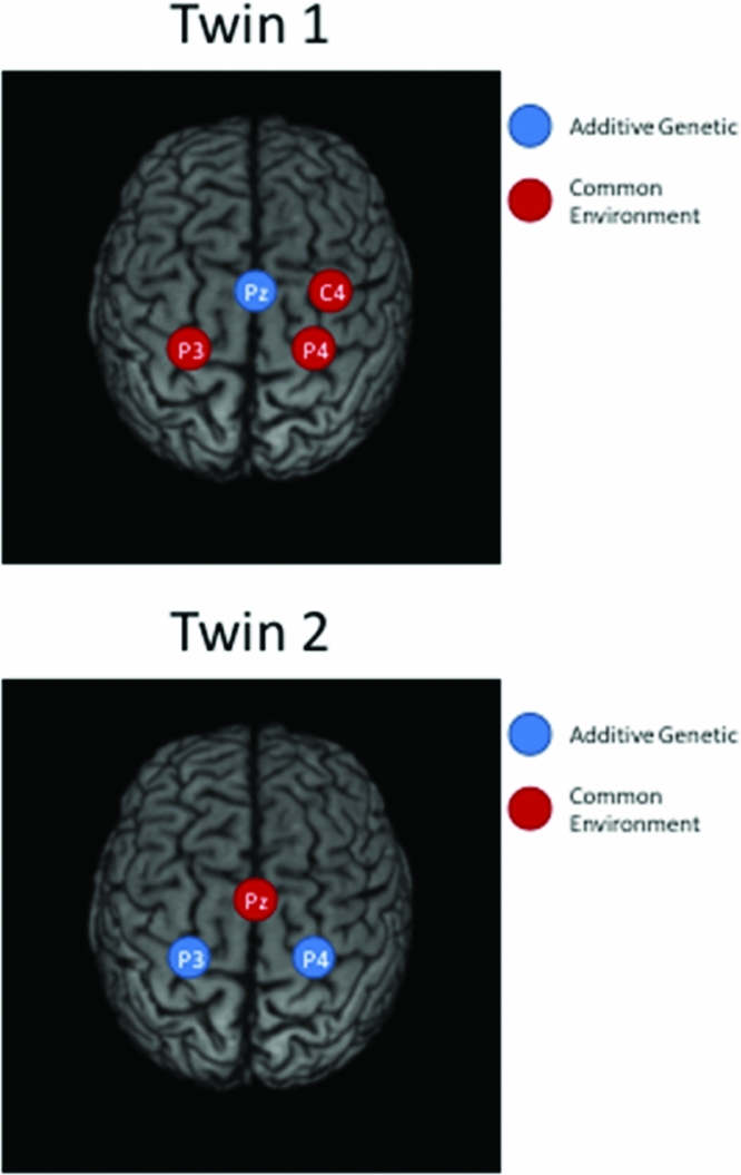
FIGURE 3 Topographic plots of the main results of iFACE applications for Twin 1 (top) and Twin 2 (bottom).
Discussion
Clearly, in this illustrative application, the homogeneity assumption is shown not to hold. The patterns of factor loadings for Twin 1 and Twin 2 differ substantially in both analyses. Similar results have been obtained with the analyses of other DZ twin pairs. These analyses are in progress and will be reported in a future publication.
The analysis presented here appears to be the first of its kind in the published literature. The results obtained should be considered to be preliminary in several respects. For instance, it is well known that multi-lead EEG is vulnerable to volume conduction effects (i.e., instantaneous conduction of the activity of each neural source throughout the brain; cf. Nunez & Srinivasan, Reference Nunez and Srinivasan2005). Volume conduction effects can be accommodated by various approaches such as basing the analysis on the current density field (the second-order spatial derivative or Laplacian of the observed potential field; cf. Nunez & Srinivasan, 2005), or fitting elementary biophysical neural source models (e.g., Grasman et al., Reference Grasman, Huizenga, Waldorp, Böcker and Molenaar2005). Also, the analysis could be applied to selected components (e.g., P300) underlying the observed event-related potentials (cf. Regan, Reference Regan1989). Please note that these qualifications only pertain to the particular field of application, but do not involve the iFACE itself.
The iFACE model can be further developed in several ways. The model fit can be carried out rather straightforwardly in the frequency domain, using the general approach presented in Molenaar (Reference Molenaar1987). Also, generalizations of the iFACE can be considered, in which factor loadings are time-varying (cf. Molenaar et al., Reference Molenaar, Sinclair, Rovine, Ram and Corneal2009), although this requires much more complex estimation techniques.
In conclusion, the iFACE (an integration of the idiographic filter and the longitudinal genetic factor model) constitutes a straightforward generalization of the standard LGFM of inter-individual variation. The formal equivalence of the iFACE and the LGFM implies equivalent formal definitions of the additive genetic, common environmental, and specific environmental factors in both models. In which way this equivalence also extends to the interpretation of these factors in the iFACE will be an important topic for future research. Presently, the main conclusion is that the iFACE provides a powerful new methodology to assess heterogeneity (subject-specificity). If the homogeneity assumption underlying standard behavior genetic analysis of inter-individual variation is thus found to be violated, its use should be critically reconsidered. We do not foresee that iFACE could provide a subject selection on an effective basis for, for example, genome-wide association studies. However, it is expected that the iFACE will help achieve a better understanding of the relationships between genetic influences and phenotypes mediated by subject-specific physiological and brain systems. This, in turn, would help foster a re-emphasis on the fundamental unit of analysis for studying behavior — the individual.
Acknowledgments
This research was funded by NSF 0852147 and NSF 1157220 to PM, Human Frontiers of Science Program RG0154/1998-B to DB, NWO/MagW VENI-451-08-026 to DS, and Award Number AG034284 from the National Institute on Aging to JN.
Supplementary materials
For supplementary material for this article, please visit http://dx.doi.org/10.1017/S1832427412000096.