


1 Introduction
An evolving magnetic field that is embedded in a highly conducting plasma generically undergoes fast magnetic reconnections, which means with a reconnection speed determined not by resistive but by Alfvénic effects (Comisso & Bhattacharjee Reference Comisso and Bhattacharjee2016; Loureiro & Uzdensky Reference Loureiro and Uzdensky2016; Zweibel & Yamada Reference Zweibel and Yamada2016). Reconnection at a speed of a tenth of the Alfvén speed is common in both observations and experiments (Comisso & Bhattacharjee Reference Comisso and Bhattacharjee2016). Since fast reconnection is both prevalent and fast compared to resistive time scales, its cause must be within the ideal evolution of magnetic fields, and this will be shown to be true. Fast magnetic reconnection is a quasi-ideal process with a conservation law, helicity conservation, which does not hold on a resistive time scale (Boozer Reference Boozer2017).
The properties of three-dimensional reconnection presented here are direct consequences of Maxwell’s equations and standard mathematics. Nevertheless, their unconventionality makes acceptance difficult. For sixty years, reconnection has been viewed as essentially a two-dimensional process even in three-dimensional space (Comisso & Bhattacharjee Reference Comisso and Bhattacharjee2016; Loureiro & Uzdensky Reference Loureiro and Uzdensky2016; Zweibel & Yamada Reference Zweibel and Yamada2016). The prevalence of fast magnetic reconnection is recognized, but the reason has not been a focus of research. Two-coordinate models can explain how reconnection can be fast but not why fast reconnection is so prevalent. The easiest way to avoid an unconventional conclusion is to not take the time to understand the derivation. To minimize that reason for avoidance, the most important derivations are placed in §§ 1 and 2 and are self-contained.
Two-coordinate systems do not naturally evolve from smooth to rapidly reconnecting states. Fast reconnection is possible in two-coordinate systems in which the initial state is singular – a state that could not naturally arise. A Harris (Reference Harris1962) sheet is a common example of such a non-realizable state (Boozer Reference Boozer2014). Another is magnetic flux ropes in which the magnetic field is strong throughout the rope but zero outside, which violates the requirement that the magnetic field not only be a continuous but also a differentiable function of position to satisfy Maxwell’s equations.
Three-coordinate models explain why magnetic reconnection is both fast and generic. Nature is three-dimensional, so two-coordinate models can only be an approximation. Three-dimensional theory is required to understand the range of validity of two-coordinate approximations.
Reconnection in this paper is defined as the changing of the connections of magnetic field lines. Consequently, there is no reconnection when a magnetic field evolves as if it were embedded in a perfectly conducting fluid moving with a velocity
 $\boldsymbol{u}$
. In this definition, the motion of magnetic field lines relative to a plasma in which they are embedded need not imply reconnection.
$\boldsymbol{u}$
. In this definition, the motion of magnetic field lines relative to a plasma in which they are embedded need not imply reconnection.
Magnetic reconnection is sometimes defined as the breaking of the ideal constraint between plasma and magnetic field line motions. For example, Eyink (Reference Eyink2015) defined magnetic reconnection by the breaking ‘of magnetic connections between plasma elements’. With this definition, fluid turbulence can enhance reconnection (Eyink, Lazarian & Vishniac Reference Eyink, Lazarian and Vishniac2011) in a way that is not possible within the definition used in this paper. One might note that the Eyink definition implies that a time-independent magnetic field in a stellarator is reconnecting as the plasma diffuses across it.
Boozer (Reference Boozer2004) noted that the evolution of a magnetic field that is embedded in a perfectly conducting fluid obeys two distinct conservation laws: (i) the ideal evolution of
 $\boldsymbol{B}$
, and (ii) the tying of the magnetic field lines to the fluid. Only the breaking of the first of these two conservation laws is relevant to reconnection as defined in this paper, and this conservation law holds far more accurately in tokamak experiments than the second, appendix A. As will be seen, plasma turbulence can enhance the breaking of magnetic connections, but as explained in § 2.1, the effect is intrinsically weaker than non-symmetric effects with a long spatial scale across the magnetic field lines.
$\boldsymbol{B}$
, and (ii) the tying of the magnetic field lines to the fluid. Only the breaking of the first of these two conservation laws is relevant to reconnection as defined in this paper, and this conservation law holds far more accurately in tokamak experiments than the second, appendix A. As will be seen, plasma turbulence can enhance the breaking of magnetic connections, but as explained in § 2.1, the effect is intrinsically weaker than non-symmetric effects with a long spatial scale across the magnetic field lines.
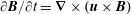
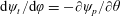
The evolution of a magnetic field is determined by the electric field,
 $\unicode[STIX]{x2202}\boldsymbol{B}/\unicode[STIX]{x2202}t=-\unicode[STIX]{x1D735}\times \boldsymbol{E}$
. The magnetic field evolution is by definition ideal wherever the electric field can be written in the form
$\unicode[STIX]{x2202}\boldsymbol{B}/\unicode[STIX]{x2202}t=-\unicode[STIX]{x1D735}\times \boldsymbol{E}$
. The magnetic field evolution is by definition ideal wherever the electric field can be written in the form
 $$\begin{eqnarray}\boldsymbol{E}+\boldsymbol{u}\times \boldsymbol{B}=-\unicode[STIX]{x1D735}\unicode[STIX]{x1D6F7},\end{eqnarray}$$
with
 $\boldsymbol{u}(\boldsymbol{x},t)$
, the magnetic field line velocity, and
$\boldsymbol{u}(\boldsymbol{x},t)$
, the magnetic field line velocity, and
 $\unicode[STIX]{x1D6F7}(\boldsymbol{x},t)$
well-behaved functions of position. Newcomb (Reference Newcomb1958) gave a proof that
$\unicode[STIX]{x1D6F7}(\boldsymbol{x},t)$
well-behaved functions of position. Newcomb (Reference Newcomb1958) gave a proof that
 $\boldsymbol{u}$
is the velocity of the magnetic field lines; Boozer (Reference Boozer2010) gave a much simpler proof. The component of
$\boldsymbol{u}$
is the velocity of the magnetic field lines; Boozer (Reference Boozer2010) gave a much simpler proof. The component of
 $\boldsymbol{u}$
along
$\boldsymbol{u}$
along
 $\boldsymbol{B}$
has no role in reconnection theory and will be assumed to be zero to simplify the discussion.
$\boldsymbol{B}$
has no role in reconnection theory and will be assumed to be zero to simplify the discussion.
Equation (1.1) implies an anti-reconnection theorem, which was first recognized by Newcomb (Reference Newcomb1958). The proof of the theorem is obvious – any vector
 $\boldsymbol{E}(\boldsymbol{x},t)$
, can be represented locally in the form of (1.1). Let
$\boldsymbol{E}(\boldsymbol{x},t)$
, can be represented locally in the form of (1.1). Let
 $\unicode[STIX]{x1D6F7}$
be a solution to
$\unicode[STIX]{x1D6F7}$
be a solution to
 $\boldsymbol{B}\boldsymbol{\cdot }\unicode[STIX]{x1D735}\unicode[STIX]{x1D6F7}=-\boldsymbol{B}\boldsymbol{\cdot }\boldsymbol{E}$
, or equivalently
$\boldsymbol{B}\boldsymbol{\cdot }\unicode[STIX]{x1D735}\unicode[STIX]{x1D6F7}=-\boldsymbol{B}\boldsymbol{\cdot }\boldsymbol{E}$
, or equivalently
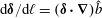
 $\text{d}\unicode[STIX]{x1D6F7}/\text{d}\ell =-E_{||}$
, where
$\text{d}\unicode[STIX]{x1D6F7}/\text{d}\ell =-E_{||}$
, where
 $\text{d}\ell$
is the differential distance along a magnetic field line. Define
$\text{d}\ell$
is the differential distance along a magnetic field line. Define
 $\boldsymbol{u}$
so
$\boldsymbol{u}$
so
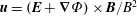 $\boldsymbol{u}=(\boldsymbol{E}+\unicode[STIX]{x1D735}\unicode[STIX]{x1D6F7})\times \boldsymbol{B}/B^{2}$
. This anti-reconnection theorem led Greene (Reference Greene1993) to the conclusion that (1.1) ‘is purely geometrical, and has no physical content’. The magnetic field line velocity
$\boldsymbol{u}=(\boldsymbol{E}+\unicode[STIX]{x1D735}\unicode[STIX]{x1D6F7})\times \boldsymbol{B}/B^{2}$
. This anti-reconnection theorem led Greene (Reference Greene1993) to the conclusion that (1.1) ‘is purely geometrical, and has no physical content’. The magnetic field line velocity
 $\boldsymbol{u}(\boldsymbol{x},t)$
is subtle but does have important physical implications. The subtlety is in the freedom of choice of the variation of
$\boldsymbol{u}(\boldsymbol{x},t)$
is subtle but does have important physical implications. The subtlety is in the freedom of choice of the variation of
 $\unicode[STIX]{x1D6F7}$
across the magnetic field lines at
$\unicode[STIX]{x1D6F7}$
across the magnetic field lines at
 $\ell =0$
when integrating
$\ell =0$
when integrating
 $\text{d}\unicode[STIX]{x1D6F7}/\text{d}\ell =-E_{||}$
. Magnetic field lines are given by a Hamiltonian, and the freedom of canonical transformations of the Hamiltonian is equivalent to the freedom in
$\text{d}\unicode[STIX]{x1D6F7}/\text{d}\ell =-E_{||}$
. Magnetic field lines are given by a Hamiltonian, and the freedom of canonical transformations of the Hamiltonian is equivalent to the freedom in
 $\unicode[STIX]{x1D6F7}$
at
$\unicode[STIX]{x1D6F7}$
at
 $\ell =0$
(Boozer Reference Boozer2004).
$\ell =0$
(Boozer Reference Boozer2004).
The separation of the velocity
 $\boldsymbol{u}$
of the magnetic field lines from the velocity
$\boldsymbol{u}$
of the magnetic field lines from the velocity
 $\boldsymbol{v}$
of the plasma and the anti-reconnection theorem remain important in relativistic theory, appendix B.
$\boldsymbol{v}$
of the plasma and the anti-reconnection theorem remain important in relativistic theory, appendix B.
Equation (1.1) implies that magnetic reconnection requires
 $\unicode[STIX]{x1D6F7}$
or
$\unicode[STIX]{x1D6F7}$
or
 $\boldsymbol{u}$
be ill behaved. As noted by Greene (Reference Greene1993), this is true at nulls of
$\boldsymbol{u}$
be ill behaved. As noted by Greene (Reference Greene1993), this is true at nulls of
 $\boldsymbol{B}$
. Nevertheless, it is difficult to understand how magnetic field nulls can explain why natural magnetic fields generically evolve into states in which fast magnetic reconnection occurs. As shown in appendix C.2, field nulls are (i) generically spatially rare, and (ii) a magnetic field line that intercepts one null does not generally intercept other nearby nulls. A field line intercepting two nulls is a more singular situation than a line intercepting only a single null. An ideal evolution without a null cannot produce a null, § 2.3. As shown by Boozer (Reference Boozer2010), in a generic evolution nulls can only be produced in pairs and only at discrete space–time points. Field nulls are clearly not required for a fast reconnection because fast magnetic reconnections are observed in tokamak plasmas, which have no magnetic nulls.
$\boldsymbol{B}$
. Nevertheless, it is difficult to understand how magnetic field nulls can explain why natural magnetic fields generically evolve into states in which fast magnetic reconnection occurs. As shown in appendix C.2, field nulls are (i) generically spatially rare, and (ii) a magnetic field line that intercepts one null does not generally intercept other nearby nulls. A field line intercepting two nulls is a more singular situation than a line intercepting only a single null. An ideal evolution without a null cannot produce a null, § 2.3. As shown by Boozer (Reference Boozer2010), in a generic evolution nulls can only be produced in pairs and only at discrete space–time points. Field nulls are clearly not required for a fast reconnection because fast magnetic reconnections are observed in tokamak plasmas, which have no magnetic nulls.
Magnetic reconnection can also occur when a well-behaved solution to
 $\text{d}\unicode[STIX]{x1D6F7}/\text{d}\ell =-E_{||}$
does not exist because of boundary conditions on the electric field. This can occur when the field lines intercept perfect conductors, or essentially equivalently when
$\text{d}\unicode[STIX]{x1D6F7}/\text{d}\ell =-E_{||}$
does not exist because of boundary conditions on the electric field. This can occur when the field lines intercept perfect conductors, or essentially equivalently when
 $\unicode[STIX]{x1D6F7}$
must obey periodicity conditions as in toroidal plasmas. Such boundary or periodicity conditions are trivially satisfied when
$\unicode[STIX]{x1D6F7}$
must obey periodicity conditions as in toroidal plasmas. Such boundary or periodicity conditions are trivially satisfied when
 $E_{||}=0$
, so a non-zero
$E_{||}=0$
, so a non-zero
 $E_{||}$
is a necessary condition for reconnection.
$E_{||}$
is a necessary condition for reconnection.
A remarkable feature of three-coordinate models is that as a magnetic field undergoes an ideal evolution, which means (1.1) is satisfied exactly, the sensitivity of field line connections to
 $E_{||}$
increases exponentially, as
$E_{||}$
increases exponentially, as
 $e^{\unicode[STIX]{x1D70E}}$
. This is due to the exponentially increasing separation of neighbouring field lines, as
$e^{\unicode[STIX]{x1D70E}}$
. This is due to the exponentially increasing separation of neighbouring field lines, as
 $e^{\unicode[STIX]{x1D70E}(\ell ,t)}$
, with distance
$e^{\unicode[STIX]{x1D70E}(\ell ,t)}$
, with distance
 $\ell$
along a line. An arbitrarily small
$\ell$
along a line. An arbitrarily small
 $E_{||}$
can produce an Alfvén speed reconnection on the overall scale of the system. This has an analogy in the mixing of fluids. Exponential separation of fluid elements in time explains the effectiveness of stirring for the intermixing of fluids, such as the stirring of cream in coffee. As explained in § 2.1, exponentiation in fluid mixing requires only two spatial coordinates but in magnetic reconnection requires three spatial coordinates.
$E_{||}$
can produce an Alfvén speed reconnection on the overall scale of the system. This has an analogy in the mixing of fluids. Exponential separation of fluid elements in time explains the effectiveness of stirring for the intermixing of fluids, such as the stirring of cream in coffee. As explained in § 2.1, exponentiation in fluid mixing requires only two spatial coordinates but in magnetic reconnection requires three spatial coordinates.
The time required for an initial magnetic field to arrive at adequate exponential sensitivity defines the trigger time for a fast reconnection. Once reconnection occurs, an Alfvénic relaxation is required before the system can re-establish a quasi-static force balance no matter how slow or weak the external drive for the magnetic field evolution may be, § 2.5. The anti-reconnection theorem, which follows from (1.1), implies the specific location of the reconnection event does not generally have a unique definition. The analogy to the trigger time in the mixing of cream into coffee is the time required for the streamers of cream to become sufficiently thin that molecular diffusion can intermix the cream and coffee on a molecular level.
No matter how slow the external forcing of an ideally evolving magnetic field may be, energy can be accumulated in the magnetic field. Much of that energy is released on a Alfvénic time scale when the exponentiation becomes sufficiently great to trigger a fast magnetic reconnection. As discussed in Boozer (Reference Boozer2017), a fast magnetic reconnection conserves magnetic helicity, which implies the full energy stored in the field cannot be released – only that associated with
 $|\unicode[STIX]{x1D735}(j_{||}/B)|$
(Woltjer Reference Woltjer1958). Equation (3.34) shows that when magnetic field lines with different
$|\unicode[STIX]{x1D735}(j_{||}/B)|$
(Woltjer Reference Woltjer1958). Equation (3.34) shows that when magnetic field lines with different
 $j_{||}/B$
are connected, a Lorentz force
$j_{||}/B$
are connected, a Lorentz force
 $\boldsymbol{f}=\boldsymbol{j}\times \boldsymbol{B}$
is exerted on the plasma. When dissipation is small, this force is balanced by the plasma inertia,
$\boldsymbol{f}=\boldsymbol{j}\times \boldsymbol{B}$
is exerted on the plasma. When dissipation is small, this force is balanced by the plasma inertia,
 $\unicode[STIX]{x1D70C}\,\text{d}\boldsymbol{v}/\text{d}t$
and the energy released by the relaxation of
$\unicode[STIX]{x1D70C}\,\text{d}\boldsymbol{v}/\text{d}t$
and the energy released by the relaxation of
 $|\unicode[STIX]{x1D735}(j_{||}/B)|$
goes into Alfvén waves. The damping of these waves transfers the energy to the plasma. This process is discussed in §§ 3 and 4.
$|\unicode[STIX]{x1D735}(j_{||}/B)|$
goes into Alfvén waves. The damping of these waves transfers the energy to the plasma. This process is discussed in §§ 3 and 4.
In three dimensions, unlike in two, the magnetic energy density
 $B^{2}/2\unicode[STIX]{x1D707}_{0}$
need not become large to obtain an arbitrarily large exponential increase when neighbouring magnetic field lines separate exponentially. Consequently, there is no natural tendency for the back reaction of the system to suppress this exponentiation. This is unlike the situation discussed by Cattaneo & Hughes (Reference Cattaneo, Hughes and Kim1996) in connection with the theory of dynamos. This is like the stirring of cream into coffee in which there is no back reaction that impedes the formation of narrow streamers of cream.
$B^{2}/2\unicode[STIX]{x1D707}_{0}$
need not become large to obtain an arbitrarily large exponential increase when neighbouring magnetic field lines separate exponentially. Consequently, there is no natural tendency for the back reaction of the system to suppress this exponentiation. This is unlike the situation discussed by Cattaneo & Hughes (Reference Cattaneo, Hughes and Kim1996) in connection with the theory of dynamos. This is like the stirring of cream into coffee in which there is no back reaction that impedes the formation of narrow streamers of cream.
Section 3.8 shows the computational difficulty of studying reconnection in three spatial dimensions increases as
 $e^{5\unicode[STIX]{x1D70E}}$
. This appears to limit direct simulations to
$e^{5\unicode[STIX]{x1D70E}}$
. This appears to limit direct simulations to
 $\unicode[STIX]{x1D70E}_{max}\approx 10$
, which is consistent with a
$\unicode[STIX]{x1D70E}_{max}\approx 10$
, which is consistent with a
 $\unicode[STIX]{x1D70E}\approx 8$
required to understand fast reconnection in fusion plasmas but much smaller than
$\unicode[STIX]{x1D70E}\approx 8$
required to understand fast reconnection in fusion plasmas but much smaller than
 $\unicode[STIX]{x1D70E}\approx 20$
required to understand reconnection in the solar corona. Simulations using modest values of
$\unicode[STIX]{x1D70E}\approx 20$
required to understand reconnection in the solar corona. Simulations using modest values of
 $\unicode[STIX]{x1D70E}$
must be sufficiently well understood to devise extrapolations or reliable approximations.
$\unicode[STIX]{x1D70E}$
must be sufficiently well understood to devise extrapolations or reliable approximations.
The computational difficulty of studying fast reconnection is sufficiently great that simplified models are required. Because exponentiation is an effect of critical importance and dominant, a simplified model, such as the one given in § 3, can answer many of the most important questions, § 4.
Models related to the model of § 3 could be used to directly study reconnection in the solar corona, § C.3, although the required number of exponentiations
 $\unicode[STIX]{x1D70E}\approx 20$
is too large for complete realism in a simulation. Such models would predict the energy of electrons in the corona and the height of the transition region to the corona. The short scale height of the plasma density below the transition region,
$\unicode[STIX]{x1D70E}\approx 20$
is too large for complete realism in a simulation. Such models would predict the energy of electrons in the corona and the height of the transition region to the corona. The short scale height of the plasma density below the transition region,
 ${\sim}100~\text{km}$
, implies that there are too few electrons to carry the current required by a quasi-ideal magnetic evolution even at a height far below the scale of magnetic phenomena on the Sun,
${\sim}100~\text{km}$
, implies that there are too few electrons to carry the current required by a quasi-ideal magnetic evolution even at a height far below the scale of magnetic phenomena on the Sun,
 ${\sim}10^{4}~\text{km}$
. Without a corona, the electron density would drop over
${\sim}10^{4}~\text{km}$
. Without a corona, the electron density would drop over
 $10^{43}$
times over a radial scale of
$10^{43}$
times over a radial scale of
 $10^{4}~\text{km}$
. Electrons runaway to whatever energy is required to carry the current, which gives a corona. This occurs where the mean free path of electrons,
$10^{4}~\text{km}$
. Electrons runaway to whatever energy is required to carry the current, which gives a corona. This occurs where the mean free path of electrons,
 $\unicode[STIX]{x1D706}_{\text{mfp}}$
, times parallel electric field becomes comparable to the local electron temperature,
$\unicode[STIX]{x1D706}_{\text{mfp}}$
, times parallel electric field becomes comparable to the local electron temperature,
 $\unicode[STIX]{x1D706}_{\text{mfp}}eE_{||}\sim T_{e}$
, where
$\unicode[STIX]{x1D706}_{\text{mfp}}eE_{||}\sim T_{e}$
, where
 $E_{||}=\unicode[STIX]{x1D702}j_{||}$
. The requirement for a corona was shown in Boozer (Reference Boozer, Brown, Canfield and Pevtsov1999) and discussed on page 1092 of Boozer (Reference Boozer2004).
$E_{||}=\unicode[STIX]{x1D702}j_{||}$
. The requirement for a corona was shown in Boozer (Reference Boozer, Brown, Canfield and Pevtsov1999) and discussed on page 1092 of Boozer (Reference Boozer2004).
The fast-reconnection mechanism explained in this paper is a clear implication of Maxwell’s equations. A different mechanism could break the ideal evolution before the exponential sensitivity to
 $E_{||}$
does. Having a definite three-coordinate model, such as the one presented in § 3, allows one to explore under what conditions the standard two-coordinate models are an adequate approximation.
$E_{||}$
does. Having a definite three-coordinate model, such as the one presented in § 3, allows one to explore under what conditions the standard two-coordinate models are an adequate approximation.
2 Ideal magnetic evolution
2.1 Exponentiation and reconnection
Magnetic field lines are defined by
 $\text{d}\boldsymbol{x}/\text{d}\ell =\hat{b}(\boldsymbol{x})$
, where
$\text{d}\boldsymbol{x}/\text{d}\ell =\hat{b}(\boldsymbol{x})$
, where
 $\hat{b}\equiv \boldsymbol{B}/|\boldsymbol{B}|$
is the unit vector and
$\hat{b}\equiv \boldsymbol{B}/|\boldsymbol{B}|$
is the unit vector and
 $\ell$
is the distance along the magnetic field. The position of a second field line is
$\ell$
is the distance along the magnetic field. The position of a second field line is
 $\boldsymbol{x}+\unicode[STIX]{x1D739}$
. By definition a neighbouring line satisfies
$\boldsymbol{x}+\unicode[STIX]{x1D739}$
. By definition a neighbouring line satisfies
 $|\unicode[STIX]{x1D739}|\rightarrow 0$
. For a neighbouring line,
$|\unicode[STIX]{x1D739}|\rightarrow 0$
. For a neighbouring line,
 $\text{d}\unicode[STIX]{x1D739}/\text{d}\ell =(\unicode[STIX]{x1D739}\boldsymbol{\cdot }\unicode[STIX]{x1D735})\hat{b}$
. This linear equation for
$\text{d}\unicode[STIX]{x1D739}/\text{d}\ell =(\unicode[STIX]{x1D739}\boldsymbol{\cdot }\unicode[STIX]{x1D735})\hat{b}$
. This linear equation for
 $\unicode[STIX]{x1D739}$
holds as long as
$\unicode[STIX]{x1D739}$
holds as long as
 $|\unicode[STIX]{x1D739}|<<a_{c}$
, where
$|\unicode[STIX]{x1D739}|<<a_{c}$
, where
 $a_{c}$
is the characteristic spatial scale within which the linear term in a Taylor expansion of
$a_{c}$
is the characteristic spatial scale within which the linear term in a Taylor expansion of
 $\hat{b}$
dominates over the higher-order terms.
$\hat{b}$
dominates over the higher-order terms.
A plasma cannot respond to maintain magnetic connectivity on a smaller spatial scale than
 $c/\unicode[STIX]{x1D714}_{\text{pe}}$
set by the inertia of the lightest charged particle, an electron. A non-ideal parallel electric field is required
$c/\unicode[STIX]{x1D714}_{\text{pe}}$
set by the inertia of the lightest charged particle, an electron. A non-ideal parallel electric field is required
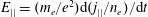 $E_{||}=(m_{e}/e^{2})\text{d}(j_{||}/n_{e})/\text{d}t$
to accelerate electrons of number density
$E_{||}=(m_{e}/e^{2})\text{d}(j_{||}/n_{e})/\text{d}t$
to accelerate electrons of number density
 $n_{e}$
to carry the required current
$n_{e}$
to carry the required current
 $j_{||}$
along the magnetic field lines;
$j_{||}$
along the magnetic field lines;
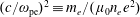 $(c/\unicode[STIX]{x1D714}_{\text{pe}})^{2}\equiv m_{e}/(\unicode[STIX]{x1D707}_{0}n_{e}e^{2})$
. In a force-free magnetic field,
$(c/\unicode[STIX]{x1D714}_{\text{pe}})^{2}\equiv m_{e}/(\unicode[STIX]{x1D707}_{0}n_{e}e^{2})$
. In a force-free magnetic field,
 $\unicode[STIX]{x1D735}\times \boldsymbol{B}=\unicode[STIX]{x1D707}_{0}\,\boldsymbol{j}_{||}$
, so when electron inertia is the only correction to the ideal evolution,
$\unicode[STIX]{x1D735}\times \boldsymbol{B}=\unicode[STIX]{x1D707}_{0}\,\boldsymbol{j}_{||}$
, so when electron inertia is the only correction to the ideal evolution,
 $$\begin{eqnarray}\frac{\unicode[STIX]{x2202}}{\unicode[STIX]{x2202}t}\left(\boldsymbol{B}-\left(\frac{c}{\unicode[STIX]{x1D714}_{\text{pe}}}\right)^{2}\unicode[STIX]{x1D6FB}^{2}\boldsymbol{B}\right)=\unicode[STIX]{x1D735}\times (\boldsymbol{u}\times \boldsymbol{B}).\end{eqnarray}$$
The
 $\unicode[STIX]{x1D6FB}^{2}\boldsymbol{B}$
term smears out the location of the magnetic field over a scale
$\unicode[STIX]{x1D6FB}^{2}\boldsymbol{B}$
term smears out the location of the magnetic field over a scale
 $c/\unicode[STIX]{x1D714}_{\text{pe}}$
. This smearing effect is seen when the right-hand side of (2.1) is replaced by resistive diffusion
$c/\unicode[STIX]{x1D714}_{\text{pe}}$
. This smearing effect is seen when the right-hand side of (2.1) is replaced by resistive diffusion
 $(\unicode[STIX]{x1D702}/\unicode[STIX]{x1D707}_{0})\unicode[STIX]{x1D6FB}^{2}\boldsymbol{B}$
, and the equation solved with
$(\unicode[STIX]{x1D702}/\unicode[STIX]{x1D707}_{0})\unicode[STIX]{x1D6FB}^{2}\boldsymbol{B}$
, and the equation solved with
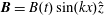 $\boldsymbol{B}=B(t)\sin (kx)\hat{z}$
. The solution is
$\boldsymbol{B}=B(t)\sin (kx)\hat{z}$
. The solution is
 $B(t)=B_{0}e^{-\unicode[STIX]{x1D708}t}$
with
$B(t)=B_{0}e^{-\unicode[STIX]{x1D708}t}$
with
 $\unicode[STIX]{x1D708}=(\unicode[STIX]{x1D702}/\unicode[STIX]{x1D707}_{0})k^{2}/(1+(c/\unicode[STIX]{x1D714}_{\text{pe}})^{2}k^{2})$
. Magnetic field lines that are within a distance of
$\unicode[STIX]{x1D708}=(\unicode[STIX]{x1D702}/\unicode[STIX]{x1D707}_{0})k^{2}/(1+(c/\unicode[STIX]{x1D714}_{\text{pe}})^{2}k^{2})$
. Magnetic field lines that are within a distance of
 $c/\unicode[STIX]{x1D714}_{\text{pe}}$
of each other at one location along their trajectories can reconnect freely even if they are separated by a distance up to
$c/\unicode[STIX]{x1D714}_{\text{pe}}$
of each other at one location along their trajectories can reconnect freely even if they are separated by a distance up to
 $a_{c}$
at some other trajectory location.
$a_{c}$
at some other trajectory location.
When the initial magnetic field is a constant,
 $B_{0}\hat{z}_{0}$
, a flux tube of circular cross-section contains flux
$B_{0}\hat{z}_{0}$
, a flux tube of circular cross-section contains flux
 $\unicode[STIX]{x03C0}B_{0}\unicode[STIX]{x1D6FF}_{0}^{2}$
, which remains fixed during an ideal evolution. In the limit
$\unicode[STIX]{x03C0}B_{0}\unicode[STIX]{x1D6FF}_{0}^{2}$
, which remains fixed during an ideal evolution. In the limit
 $\unicode[STIX]{x1D6FF}_{0}\rightarrow 0$
, the tube evolves into an elliptical cross-section with major and minor radii
$\unicode[STIX]{x1D6FF}_{0}\rightarrow 0$
, the tube evolves into an elliptical cross-section with major and minor radii
 $\unicode[STIX]{x1D6FF}_{\text{maj}}$
and
$\unicode[STIX]{x1D6FF}_{\text{maj}}$
and
 $\unicode[STIX]{x1D6FF}_{\text{min}}$
but with the same flux,
$\unicode[STIX]{x1D6FF}_{\text{min}}$
but with the same flux,
 $\unicode[STIX]{x03C0}B\unicode[STIX]{x1D6FF}_{\text{maj}}\unicode[STIX]{x1D6FF}_{\text{min}}=\unicode[STIX]{x03C0}B_{0}\unicode[STIX]{x1D6FF}_{0}^{2}$
. The major radius grows as
$\unicode[STIX]{x03C0}B\unicode[STIX]{x1D6FF}_{\text{maj}}\unicode[STIX]{x1D6FF}_{\text{min}}=\unicode[STIX]{x03C0}B_{0}\unicode[STIX]{x1D6FF}_{0}^{2}$
. The major radius grows as
 $\unicode[STIX]{x1D6FF}_{\text{maj}}=\unicode[STIX]{x1D6FF}_{0}e^{\unicode[STIX]{x1D70E}(\ell ,t)}$
with time and distance along the tube, where
$\unicode[STIX]{x1D6FF}_{\text{maj}}=\unicode[STIX]{x1D6FF}_{0}e^{\unicode[STIX]{x1D70E}(\ell ,t)}$
with time and distance along the tube, where
 $\unicode[STIX]{x1D70E}$
is a Lyapunov exponent associated with the flow
$\unicode[STIX]{x1D70E}$
is a Lyapunov exponent associated with the flow
 $\boldsymbol{u}$
. A precise definition of
$\boldsymbol{u}$
. A precise definition of
 $\unicode[STIX]{x1D70E}$
is given in § 2.3. The minor radius must shrink as
$\unicode[STIX]{x1D70E}$
is given in § 2.3. The minor radius must shrink as
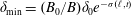 $\unicode[STIX]{x1D6FF}_{\text{min}}=(B_{0}/B)\unicode[STIX]{x1D6FF}_{0}e^{-\unicode[STIX]{x1D70E}(\ell ,t)}$
. When the initial radius
$\unicode[STIX]{x1D6FF}_{\text{min}}=(B_{0}/B)\unicode[STIX]{x1D6FF}_{0}e^{-\unicode[STIX]{x1D70E}(\ell ,t)}$
. When the initial radius
 $\unicode[STIX]{x1D6FF}_{0}$
is made finite, the major radius can become larger than the characteristic spatial scale
$\unicode[STIX]{x1D6FF}_{0}$
is made finite, the major radius can become larger than the characteristic spatial scale
 $a_{c}$
. When
$a_{c}$
. When
 $\unicode[STIX]{x1D6FF}_{\text{maj}}$
becomes greater than
$\unicode[STIX]{x1D6FF}_{\text{maj}}$
becomes greater than
 $a_{c}$
, the flux tube deforms into an extremely complicated shape and the maximum distance between points in a cross-section of the flux tube increases only as
$a_{c}$
, the flux tube deforms into an extremely complicated shape and the maximum distance between points in a cross-section of the flux tube increases only as
 $\ell$
to a power, which is the case considered by Rechester & Rosenbluth (Reference Rechester and Rosenbluth1978). For this reason, short wavelength plasma turbulence intrinsically produces a less dramatic increase in the reconnection rate than the exponential increase caused by variations in the field of longer wavelength. For spatial scales
$\ell$
to a power, which is the case considered by Rechester & Rosenbluth (Reference Rechester and Rosenbluth1978). For this reason, short wavelength plasma turbulence intrinsically produces a less dramatic increase in the reconnection rate than the exponential increase caused by variations in the field of longer wavelength. For spatial scales
 $a<a_{c}$
, fast magnetic reconnection can occur over the scale
$a<a_{c}$
, fast magnetic reconnection can occur over the scale
 $a$
when the change in the exponentiation along a magnetic field line
$a$
when the change in the exponentiation along a magnetic field line
 $\unicode[STIX]{x1D6FF}\unicode[STIX]{x1D70E}$
satisfies
$\unicode[STIX]{x1D6FF}\unicode[STIX]{x1D70E}$
satisfies
 $\unicode[STIX]{x1D6FF}\unicode[STIX]{x1D70E}\sim \ln (a/(c/\unicode[STIX]{x1D714}_{\text{pe}}))$
.
$\unicode[STIX]{x1D6FF}\unicode[STIX]{x1D70E}\sim \ln (a/(c/\unicode[STIX]{x1D714}_{\text{pe}}))$
.
The transition in the form of the separation of magnetic field lines from exponential when
 $\unicode[STIX]{x1D6FF}_{\text{maj}}<a_{c}$
to a power-law,
$\unicode[STIX]{x1D6FF}_{\text{maj}}<a_{c}$
to a power-law,
 $\ell ^{\unicode[STIX]{x1D6FC}}$
, is complicated. Analogous issues arise in the mixing of fluids and its practical applications – even stirring cream in coffee. Two articles in the Reviews of Modern Physics help clarify the issues. The limit corresponding to
$\ell ^{\unicode[STIX]{x1D6FC}}$
, is complicated. Analogous issues arise in the mixing of fluids and its practical applications – even stirring cream in coffee. Two articles in the Reviews of Modern Physics help clarify the issues. The limit corresponding to
 $\unicode[STIX]{x1D6FF}_{\text{maj}}<a_{c}$
is the advective or stirring limit for fluids and the opposite limit is the mixing or turbulent limit. Both reviews consider the two limits. The earlier review of Falkovich, Gawdcezki & Vergassola (Reference Falkovich, Gawdȩzki and Vergassola2001) emphasized the turbulent limit and a recent review by Aref et al. (Reference Aref, Blake, Budisić, Cardoso, Cartwright, Clercx, El Omari, Feudel, Golestanian and Gouillart2017) emphasized the advective limit. Separations between fluid elements typically increase exponentially with time in the advective limit but as time to a power in turbulent limit. Different powers of time arise depending on assumptions. Numerical studies of the field line motion in models of turbulent magnetic fields were given in Zimbardo et al. (Reference Zimbardo, Veltri, Basile and Principato1995). The separation between neighbouring magnetic field lines were observed to increase as a power law,
$\unicode[STIX]{x1D6FF}_{\text{maj}}<a_{c}$
is the advective or stirring limit for fluids and the opposite limit is the mixing or turbulent limit. Both reviews consider the two limits. The earlier review of Falkovich, Gawdcezki & Vergassola (Reference Falkovich, Gawdȩzki and Vergassola2001) emphasized the turbulent limit and a recent review by Aref et al. (Reference Aref, Blake, Budisić, Cardoso, Cartwright, Clercx, El Omari, Feudel, Golestanian and Gouillart2017) emphasized the advective limit. Separations between fluid elements typically increase exponentially with time in the advective limit but as time to a power in turbulent limit. Different powers of time arise depending on assumptions. Numerical studies of the field line motion in models of turbulent magnetic fields were given in Zimbardo et al. (Reference Zimbardo, Veltri, Basile and Principato1995). The separation between neighbouring magnetic field lines were observed to increase as a power law,
 $\ell ^{\unicode[STIX]{x1D6FC}}$
, with the power depending on the assumptions of the model.
$\ell ^{\unicode[STIX]{x1D6FC}}$
, with the power depending on the assumptions of the model.
An important distinction exists between mixing in a two-coordinate model of an incompressible flow, such as
 $\boldsymbol{v}=\unicode[STIX]{x1D735}\unicode[STIX]{x1D719}(x,y,t)\times \hat{z}$
, and reconnection in a two-coordinate model of the magnetic field, such as
$\boldsymbol{v}=\unicode[STIX]{x1D735}\unicode[STIX]{x1D719}(x,y,t)\times \hat{z}$
, and reconnection in a two-coordinate model of the magnetic field, such as
 $\boldsymbol{B}=B_{g}(\hat{z}+\unicode[STIX]{x1D735}H(x,y,t)\times \hat{z})$
, where
$\boldsymbol{B}=B_{g}(\hat{z}+\unicode[STIX]{x1D735}H(x,y,t)\times \hat{z})$
, where
 $B_{g}$
is a strong and constant guide field. Both streamlines and magnetic field lines obey Hamilton’s equations. For streamlines,
$B_{g}$
is a strong and constant guide field. Both streamlines and magnetic field lines obey Hamilton’s equations. For streamlines,
 $\text{d}x/\text{d}t=\unicode[STIX]{x2202}\unicode[STIX]{x1D719}/\unicode[STIX]{x2202}y$
and
$\text{d}x/\text{d}t=\unicode[STIX]{x2202}\unicode[STIX]{x1D719}/\unicode[STIX]{x2202}y$
and
 $\text{d}y/\text{d}t=-\unicode[STIX]{x2202}\unicode[STIX]{x1D719}/\unicode[STIX]{x2202}x$
. For magnetic field lines,
$\text{d}y/\text{d}t=-\unicode[STIX]{x2202}\unicode[STIX]{x1D719}/\unicode[STIX]{x2202}x$
. For magnetic field lines,
 $\text{d}x/\text{d}z=\unicode[STIX]{x2202}H/\unicode[STIX]{x2202}y$
and
$\text{d}x/\text{d}z=\unicode[STIX]{x2202}H/\unicode[STIX]{x2202}y$
and
 $\text{d}y/\text{d}z=-\unicode[STIX]{x2202}H/\unicode[STIX]{x2202}x$
, so
$\text{d}y/\text{d}z=-\unicode[STIX]{x2202}H/\unicode[STIX]{x2202}x$
, so
 $\text{d}H/\text{d}z=(\unicode[STIX]{x2202}H/\unicode[STIX]{x2202}x)(\text{d}x/\text{d}z)+(\unicode[STIX]{x2202}H/\unicode[STIX]{x2202}y)(\text{d}y/\text{d}z)=0$
. With only two coordinates, a magnetic field line must follow a constant-
$\text{d}H/\text{d}z=(\unicode[STIX]{x2202}H/\unicode[STIX]{x2202}x)(\text{d}x/\text{d}z)+(\unicode[STIX]{x2202}H/\unicode[STIX]{x2202}y)(\text{d}y/\text{d}z)=0$
. With only two coordinates, a magnetic field line must follow a constant-
 $H$
contour. No such constraint applies to streamlines in a time-dependent flow. Although a rapid mixing of fluids can occur with time-dependent stirring in a two-coordinate model, a three-coordinate model is required for the analogous effect to enhance magnetic reconnection.
$H$
contour. No such constraint applies to streamlines in a time-dependent flow. Although a rapid mixing of fluids can occur with time-dependent stirring in a two-coordinate model, a three-coordinate model is required for the analogous effect to enhance magnetic reconnection.
In the solar corona,
 $c/\unicode[STIX]{x1D714}_{\text{pe}}\sim 10~\text{cm}$
, and the radius of the Sun is approximately ten orders of magnitude greater,
$c/\unicode[STIX]{x1D714}_{\text{pe}}\sim 10~\text{cm}$
, and the radius of the Sun is approximately ten orders of magnitude greater,
 $R_{\odot }\approx 7\times 10^{5}~\text{km}$
, so an exponentiation
$R_{\odot }\approx 7\times 10^{5}~\text{km}$
, so an exponentiation
 $\unicode[STIX]{x1D70E}\sim 23$
could be responsible for all observed reconnection events. An even larger
$\unicode[STIX]{x1D70E}\sim 23$
could be responsible for all observed reconnection events. An even larger
 $\unicode[STIX]{x1D70E}$
may arise in astrophysical reconnection. A much smaller
$\unicode[STIX]{x1D70E}$
may arise in astrophysical reconnection. A much smaller
 $\unicode[STIX]{x1D70E}$
is required to explain fast reconnections in fusion experiments. The minor radius of ITER is
$\unicode[STIX]{x1D70E}$
is required to explain fast reconnections in fusion experiments. The minor radius of ITER is
 $a=2.0~\text{m}$
, and the standard operating density is
$a=2.0~\text{m}$
, and the standard operating density is
 $10^{20}~\text{electrons m}^{-3}$
, which makes
$10^{20}~\text{electrons m}^{-3}$
, which makes
 $a/(c/\unicode[STIX]{x1D714}_{\text{pe}})=e^{8.2}$
.
$a/(c/\unicode[STIX]{x1D714}_{\text{pe}})=e^{8.2}$
.
2.2 Ideal form for
 $\boldsymbol{B}(\boldsymbol{x},t)$

A magnetic field
 $\boldsymbol{B}(\boldsymbol{x},t)$
maintains a special form, equation (2.8), when it is undergoing an arbitrary ideal evolution from an initial state
$\boldsymbol{B}(\boldsymbol{x},t)$
maintains a special form, equation (2.8), when it is undergoing an arbitrary ideal evolution from an initial state
 $\boldsymbol{B}_{0}(\boldsymbol{x}_{0})$
. This form is based on the transformation to Lagrangian coordinates,
$\boldsymbol{B}_{0}(\boldsymbol{x}_{0})$
. This form is based on the transformation to Lagrangian coordinates,
 $\boldsymbol{x}(\boldsymbol{x}_{0},t)$
,
$\boldsymbol{x}(\boldsymbol{x}_{0},t)$
,
 $$\begin{eqnarray}\frac{\text{d}\boldsymbol{x}}{\text{d}t}\equiv \boldsymbol{u}(\boldsymbol{x},t),\end{eqnarray}$$
with the initial condition
 $\boldsymbol{x}(\boldsymbol{x}_{0},t_{0})=\boldsymbol{x}_{0}$
and with
$\boldsymbol{x}(\boldsymbol{x}_{0},t_{0})=\boldsymbol{x}_{0}$
and with
 $\boldsymbol{u}(\boldsymbol{x},t)$
the velocity in (1.1). When
$\boldsymbol{u}(\boldsymbol{x},t)$
the velocity in (1.1). When
 $f(\boldsymbol{x},t)$
is an arbitrary function,
$f(\boldsymbol{x},t)$
is an arbitrary function,
 $\text{d}f/\text{d}t\equiv \unicode[STIX]{x2202}f/\unicode[STIX]{x2202}t+\boldsymbol{u}\boldsymbol{\cdot }\unicode[STIX]{x1D735}f$
. Since
$\text{d}f/\text{d}t\equiv \unicode[STIX]{x2202}f/\unicode[STIX]{x2202}t+\boldsymbol{u}\boldsymbol{\cdot }\unicode[STIX]{x1D735}f$
. Since
 $\boldsymbol{x}_{0}$
is not changed by the flow,
$\boldsymbol{x}_{0}$
is not changed by the flow,
 $\text{d}f/\text{d}t=(\unicode[STIX]{x2202}f/\unicode[STIX]{x2202}t)_{\boldsymbol{x}_{0}}$
.
$\text{d}f/\text{d}t=(\unicode[STIX]{x2202}f/\unicode[STIX]{x2202}t)_{\boldsymbol{x}_{0}}$
.
The Jacobian matrix of the coordinate transformation
 $\boldsymbol{x}(\boldsymbol{x}_{0},t)$
is
$\boldsymbol{x}(\boldsymbol{x}_{0},t)$
is
 $$\begin{eqnarray}\unicode[STIX]{x1D645}\equiv \frac{\unicode[STIX]{x2202}\boldsymbol{x}}{\unicode[STIX]{x2202}\boldsymbol{x}_{0}}\equiv \left(\begin{array}{@{}ccc@{}}\displaystyle \frac{\unicode[STIX]{x2202}x}{\unicode[STIX]{x2202}x_{0}} & \displaystyle \frac{\unicode[STIX]{x2202}x}{\unicode[STIX]{x2202}y_{0}} & \displaystyle \frac{\unicode[STIX]{x2202}x}{\unicode[STIX]{x2202}z_{0}}\\ \displaystyle \frac{\unicode[STIX]{x2202}y}{\unicode[STIX]{x2202}x_{0}} & \displaystyle \frac{\unicode[STIX]{x2202}y}{\unicode[STIX]{x2202}y_{0}} & \displaystyle \frac{\unicode[STIX]{x2202}y}{\unicode[STIX]{x2202}z_{0}}\\ \displaystyle \frac{\unicode[STIX]{x2202}z}{\unicode[STIX]{x2202}x_{0}} & \displaystyle \frac{\unicode[STIX]{x2202}z}{\unicode[STIX]{x2202}y_{0}} & \displaystyle \frac{\unicode[STIX]{x2202}z}{\unicode[STIX]{x2202}z_{0}}\end{array}\right).\end{eqnarray}$$
The Jacobian
 ${\mathcal{J}}$
is the determinant of the Jacobian matrix,
${\mathcal{J}}$
is the determinant of the Jacobian matrix,
 ${\mathcal{J}}\equiv \left|\unicode[STIX]{x1D645}\right|$
.
${\mathcal{J}}\equiv \left|\unicode[STIX]{x1D645}\right|$
.
The time derivative of the Jacobian can be derived using an arbitrary volume moving with the flow,
 $V\equiv \int {\mathcal{J}}\text{d}^{3}x_{0}$
. This volume changes as
$V\equiv \int {\mathcal{J}}\text{d}^{3}x_{0}$
. This volume changes as
 $\text{d}V/\text{d}t=\oint \boldsymbol{u}\boldsymbol{\cdot }\text{d}\boldsymbol{a}=\int \unicode[STIX]{x1D735}\boldsymbol{\cdot }\boldsymbol{u}\text{d}^{3}x=\int \unicode[STIX]{x1D735}\boldsymbol{\cdot }\boldsymbol{u}{\mathcal{J}}\text{d}^{3}x_{0}$
. Since
$\text{d}V/\text{d}t=\oint \boldsymbol{u}\boldsymbol{\cdot }\text{d}\boldsymbol{a}=\int \unicode[STIX]{x1D735}\boldsymbol{\cdot }\boldsymbol{u}\text{d}^{3}x=\int \unicode[STIX]{x1D735}\boldsymbol{\cdot }\boldsymbol{u}{\mathcal{J}}\text{d}^{3}x_{0}$
. Since
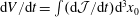 $\text{d}V/\text{d}t=\int (\text{d}{\mathcal{J}}/\text{d}t)\text{d}^{3}x_{0}$
holds for an arbitrary volume,
$\text{d}V/\text{d}t=\int (\text{d}{\mathcal{J}}/\text{d}t)\text{d}^{3}x_{0}$
holds for an arbitrary volume,
 $$\begin{eqnarray}\frac{\text{d}{\mathcal{J}}}{\text{d}t}={\mathcal{J}}\unicode[STIX]{x1D735}\boldsymbol{\cdot }\boldsymbol{u}.\end{eqnarray}$$
In an ideal evolution,
 $\unicode[STIX]{x2202}\boldsymbol{B}/\unicode[STIX]{x2202}t=\unicode[STIX]{x1D735}\times (\boldsymbol{u}\times \boldsymbol{B})=-\boldsymbol{B}\unicode[STIX]{x1D735}\boldsymbol{\cdot }\boldsymbol{u}+\boldsymbol{B}\boldsymbol{\cdot }\unicode[STIX]{x1D735}\boldsymbol{u}-\boldsymbol{u}\boldsymbol{\cdot }\unicode[STIX]{x1D735}\boldsymbol{B}$
, so
$\unicode[STIX]{x2202}\boldsymbol{B}/\unicode[STIX]{x2202}t=\unicode[STIX]{x1D735}\times (\boldsymbol{u}\times \boldsymbol{B})=-\boldsymbol{B}\unicode[STIX]{x1D735}\boldsymbol{\cdot }\boldsymbol{u}+\boldsymbol{B}\boldsymbol{\cdot }\unicode[STIX]{x1D735}\boldsymbol{u}-\boldsymbol{u}\boldsymbol{\cdot }\unicode[STIX]{x1D735}\boldsymbol{B}$
, so
 $$\begin{eqnarray}\displaystyle \frac{\text{d}({\mathcal{J}}\boldsymbol{B})}{\text{d}t}=({\mathcal{J}}\boldsymbol{B})\boldsymbol{\cdot }\unicode[STIX]{x1D735}\boldsymbol{u}. & & \displaystyle\end{eqnarray}$$
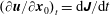
The general expression for
 $\boldsymbol{B}\boldsymbol{\cdot }\unicode[STIX]{x1D735}f$
is apparent from its two-coordinate form
$\boldsymbol{B}\boldsymbol{\cdot }\unicode[STIX]{x1D735}f$
is apparent from its two-coordinate form
 $$\begin{eqnarray}\displaystyle \boldsymbol{B}\boldsymbol{\cdot }\unicode[STIX]{x1D735}f & = & \displaystyle B_{x}\left(\frac{\unicode[STIX]{x2202}x_{0}}{\unicode[STIX]{x2202}x}\frac{\unicode[STIX]{x2202}}{\unicode[STIX]{x2202}x_{0}}+\frac{\unicode[STIX]{x2202}y_{0}}{\unicode[STIX]{x2202}x}\frac{\unicode[STIX]{x2202}}{\unicode[STIX]{x2202}y_{0}}\right)fB_{y}\left(\frac{\unicode[STIX]{x2202}x_{0}}{\unicode[STIX]{x2202}y}\frac{\unicode[STIX]{x2202}}{\unicode[STIX]{x2202}x_{0}}+\frac{\unicode[STIX]{x2202}y_{0}}{\unicode[STIX]{x2202}y}\frac{\unicode[STIX]{x2202}}{\unicode[STIX]{x2202}y_{0}}\right)f\nonumber\\ \displaystyle & = & \displaystyle \frac{\unicode[STIX]{x2202}f}{\unicode[STIX]{x2202}\boldsymbol{x}_{0}}\boldsymbol{\cdot }\frac{\unicode[STIX]{x2202}\boldsymbol{x}_{0}}{\unicode[STIX]{x2202}\boldsymbol{x}}\boldsymbol{\cdot }\boldsymbol{B}\end{eqnarray}$$
as is
 $\unicode[STIX]{x1D645}^{-1}=\unicode[STIX]{x2202}\boldsymbol{x}_{0}/\unicode[STIX]{x2202}\boldsymbol{x}$
. Since
$\unicode[STIX]{x1D645}^{-1}=\unicode[STIX]{x2202}\boldsymbol{x}_{0}/\unicode[STIX]{x2202}\boldsymbol{x}$
. Since
 $\boldsymbol{u}\equiv \unicode[STIX]{x2202}\boldsymbol{x}(\boldsymbol{x}_{0},t)/\unicode[STIX]{x2202}t$
, the derivative
$\boldsymbol{u}\equiv \unicode[STIX]{x2202}\boldsymbol{x}(\boldsymbol{x}_{0},t)/\unicode[STIX]{x2202}t$
, the derivative
 $(\unicode[STIX]{x2202}\boldsymbol{u}/\unicode[STIX]{x2202}\boldsymbol{x}_{0})_{t}=\text{d}\unicode[STIX]{x1D645}/\text{d}t$
. Therefore, equation (2.5) is equivalent to
$(\unicode[STIX]{x2202}\boldsymbol{u}/\unicode[STIX]{x2202}\boldsymbol{x}_{0})_{t}=\text{d}\unicode[STIX]{x1D645}/\text{d}t$
. Therefore, equation (2.5) is equivalent to
 $$\begin{eqnarray}\frac{\text{d}({\mathcal{J}}\boldsymbol{B})}{\text{d}t}=\frac{\text{d}\unicode[STIX]{x1D645}}{\text{d}t}\boldsymbol{\cdot }\unicode[STIX]{x1D645}^{-1}\boldsymbol{\cdot }({\mathcal{J}}\boldsymbol{B}),\end{eqnarray}$$
which is solved by
 $$\begin{eqnarray}\displaystyle \boldsymbol{B}(\boldsymbol{x},t)=\frac{\unicode[STIX]{x1D645}}{{\mathcal{J}}}\boldsymbol{\cdot }\boldsymbol{B}_{0}(\boldsymbol{x}_{0}), & & \displaystyle\end{eqnarray}$$
where
 $\boldsymbol{B}_{0}(\boldsymbol{x}_{0})$
is the initial,
$\boldsymbol{B}_{0}(\boldsymbol{x}_{0})$
is the initial,
 $t=t_{0}$
, magnetic field. Equation (2.8) is given in the review of reconnection by Zweibel & Yamada (Reference Zweibel and Yamada2016). The long history of this equation was discussed by Stern (Reference Stern1966). Zweibel (Reference Zweibel1998) used (2.8) to study magnetic reconnection when there is a stagnation point in the plasma flow. Her analysis is related to that given in § 2.3 for the effect on reconnection of a generic magnetic field line velocity.
$t=t_{0}$
, magnetic field. Equation (2.8) is given in the review of reconnection by Zweibel & Yamada (Reference Zweibel and Yamada2016). The long history of this equation was discussed by Stern (Reference Stern1966). Zweibel (Reference Zweibel1998) used (2.8) to study magnetic reconnection when there is a stagnation point in the plasma flow. Her analysis is related to that given in § 2.3 for the effect on reconnection of a generic magnetic field line velocity.
2.3 Ideal
$\boldsymbol{B}(\boldsymbol{x},t)$
and exponentiation

The Jacobian matrix can be written using a singular value decomposition (SVD), as can any three-by-three matrix with real coefficients,
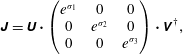 $$\begin{eqnarray}\unicode[STIX]{x1D645}=\unicode[STIX]{x1D650}\boldsymbol{\cdot }\left(\begin{array}{@{}ccc@{}}e^{\unicode[STIX]{x1D70E}_{1}} & 0 & 0\\ 0 & e^{\unicode[STIX]{x1D70E}_{2}} & 0\\ 0 & 0 & e^{\unicode[STIX]{x1D70E}_{3}}\end{array}\right)\boldsymbol{\cdot }\unicode[STIX]{x1D651}^{\dagger },\end{eqnarray}$$
where
 $\unicode[STIX]{x1D650}$
and
$\unicode[STIX]{x1D650}$
and
 $\unicode[STIX]{x1D651}$
are orthogonal matrices,
$\unicode[STIX]{x1D651}$
are orthogonal matrices,
 $\unicode[STIX]{x1D650}^{\dagger }\boldsymbol{\cdot }\unicode[STIX]{x1D650}=\mathbf{1}$
. Orthogonal matrices give rotations. This is obvious for a two-by-two orthogonal matrix, which has the general form
$\unicode[STIX]{x1D650}^{\dagger }\boldsymbol{\cdot }\unicode[STIX]{x1D650}=\mathbf{1}$
. Orthogonal matrices give rotations. This is obvious for a two-by-two orthogonal matrix, which has the general form
 $$\begin{eqnarray}\unicode[STIX]{x1D650}=\left(\begin{array}{@{}cc@{}}\cos \unicode[STIX]{x1D6FC} & \sin \unicode[STIX]{x1D6FC}\\ -\sin \unicode[STIX]{x1D6FC} & \cos \unicode[STIX]{x1D6FC}\end{array}\right)\end{eqnarray}$$
when
 $\unicode[STIX]{x1D650}$
goes to the identity matrix as the rotation angle
$\unicode[STIX]{x1D650}$
goes to the identity matrix as the rotation angle
 $\unicode[STIX]{x1D6FC}$
goes to zero. In an SVD analysis, the coefficients
$\unicode[STIX]{x1D6FC}$
goes to zero. In an SVD analysis, the coefficients
 $e^{\unicode[STIX]{x1D70E}_{1}}$
,
$e^{\unicode[STIX]{x1D70E}_{1}}$
,
 $e^{\unicode[STIX]{x1D70E}_{2}}$
and
$e^{\unicode[STIX]{x1D70E}_{2}}$
and
 $e^{\unicode[STIX]{x1D70E}_{3}}$
are called singular values and are positive real numbers. In the theory of dynamical systems, the real numbers
$e^{\unicode[STIX]{x1D70E}_{3}}$
are called singular values and are positive real numbers. In the theory of dynamical systems, the real numbers
 $\unicode[STIX]{x1D70E}_{1-3}$
are known as Lyapunov exponents, or more precisely as finite-time Lyapunov exponents.
$\unicode[STIX]{x1D70E}_{1-3}$
are known as Lyapunov exponents, or more precisely as finite-time Lyapunov exponents.
The dot product of the magnetic field with itself implies
 $$\begin{eqnarray}\left(\frac{{\mathcal{J}}B}{B_{0}}\right)^{2}=\hat{b}_{0}^{\dagger }\boldsymbol{\cdot }\unicode[STIX]{x1D651}\boldsymbol{\cdot }\left(\begin{array}{@{}ccc@{}}e^{2\unicode[STIX]{x1D70E}_{1}} & 0 & 0\\ 0 & e^{2\unicode[STIX]{x1D70E}_{2}} & 0\\ 0 & 0 & e^{2\unicode[STIX]{x1D70E}_{3}}\end{array}\right)\boldsymbol{\cdot }\unicode[STIX]{x1D651}^{\dagger }\boldsymbol{\cdot }\hat{b}_{0},\end{eqnarray}$$
where
 $\hat{b}_{0}=\boldsymbol{B}_{0}/B_{0}$
is the unit vector along the initial magnetic field.
$\hat{b}_{0}=\boldsymbol{B}_{0}/B_{0}$
is the unit vector along the initial magnetic field.
The component of
 $\boldsymbol{u}$
that is parallel to the magnetic field does not appear in (1.1) for an ideal evolution and is taken to be zero, which simplifies the analysis, especially in relativistic theory. With
$\boldsymbol{u}$
that is parallel to the magnetic field does not appear in (1.1) for an ideal evolution and is taken to be zero, which simplifies the analysis, especially in relativistic theory. With
 $\boldsymbol{u}\boldsymbol{\cdot }\boldsymbol{B}=0$
, magnetic flux conservation during the evolution then implies
$\boldsymbol{u}\boldsymbol{\cdot }\boldsymbol{B}=0$
, magnetic flux conservation during the evolution then implies
 ${\mathcal{J}}B=B_{0}$
.
${\mathcal{J}}B=B_{0}$
.
Define the transformed unit vector
 $\hat{b}_{t}\equiv \unicode[STIX]{x1D651}^{\dagger }\boldsymbol{\cdot }\hat{b}_{0}$
, then
$\hat{b}_{t}\equiv \unicode[STIX]{x1D651}^{\dagger }\boldsymbol{\cdot }\hat{b}_{0}$
, then
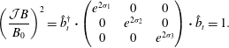 $$\begin{eqnarray}\left(\frac{{\mathcal{J}}B}{B_{0}}\right)^{2}=\hat{b}_{t}^{\dagger }\boldsymbol{\cdot }\left(\begin{array}{@{}ccc@{}}e^{2\unicode[STIX]{x1D70E}_{1}} & 0 & 0\\ 0 & e^{2\unicode[STIX]{x1D70E}_{2}} & 0\\ 0 & 0 & e^{2\unicode[STIX]{x1D70E}_{3}}\end{array}\right)\boldsymbol{\cdot }\hat{b}_{t}=1.\end{eqnarray}$$
One of the singular values, which will be taken to be
 $e^{\unicode[STIX]{x1D70E}_{3}}$
, must be unity, and
$e^{\unicode[STIX]{x1D70E}_{3}}$
, must be unity, and
 $\hat{b}_{t}$
is the associated eigenvector. Consequently,
$\hat{b}_{t}$
is the associated eigenvector. Consequently,
 $$\begin{eqnarray}\displaystyle \unicode[STIX]{x1D645} & = & \displaystyle \unicode[STIX]{x1D650}\boldsymbol{\cdot }\left(\begin{array}{@{}ccc@{}}e^{\unicode[STIX]{x1D70E}_{1}} & 0 & 0\\ 0 & e^{\unicode[STIX]{x1D70E}_{2}} & 0\\ 0 & 0 & 1\end{array}\right)\boldsymbol{\cdot }\unicode[STIX]{x1D651}^{\dagger };\end{eqnarray}$$
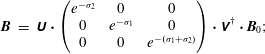 $$\begin{eqnarray}\displaystyle \boldsymbol{B} & = & \displaystyle \unicode[STIX]{x1D650}\boldsymbol{\cdot }\left(\begin{array}{@{}ccc@{}}e^{-\unicode[STIX]{x1D70E}_{2}} & 0 & 0\\ 0 & e^{-\unicode[STIX]{x1D70E}_{1}} & 0\\ 0 & 0 & e^{-(\unicode[STIX]{x1D70E}_{1}+\unicode[STIX]{x1D70E}_{2})}\end{array}\right)\boldsymbol{\cdot }\unicode[STIX]{x1D651}^{\dagger }\boldsymbol{\cdot }\boldsymbol{B}_{0};\end{eqnarray}$$
 $$\begin{eqnarray}\displaystyle B & = & \displaystyle \frac{B_{0}}{{\mathcal{J}}}=B_{0}e^{-(\unicode[STIX]{x1D70E}_{1}+\unicode[STIX]{x1D70E}_{2})}.\end{eqnarray}$$
The magnetic field strength can change in an ideal evolution, but only exponentially, which is not consistent with the formation of a null where none existed before.
2.4 Ideal evolution of the current density
The parallel-current density, which is the component that is directly involved in reconnection, generally increases as the magnetic field evolves. The current density
 $\boldsymbol{j}=\unicode[STIX]{x1D735}\times (B\hat{b})/\unicode[STIX]{x1D707}_{0}=(\unicode[STIX]{x1D735}B/\unicode[STIX]{x1D707}_{0})\times \hat{b}+(B/\unicode[STIX]{x1D707}_{0})\unicode[STIX]{x1D735}\times \hat{b}$
, so
$\boldsymbol{j}=\unicode[STIX]{x1D735}\times (B\hat{b})/\unicode[STIX]{x1D707}_{0}=(\unicode[STIX]{x1D735}B/\unicode[STIX]{x1D707}_{0})\times \hat{b}+(B/\unicode[STIX]{x1D707}_{0})\unicode[STIX]{x1D735}\times \hat{b}$
, so
 $$\begin{eqnarray}\displaystyle K & \equiv & \displaystyle \frac{\unicode[STIX]{x1D707}_{0}j_{||}}{B}\end{eqnarray}$$
 $$\begin{eqnarray}\displaystyle & = & \displaystyle \hat{b}\boldsymbol{\cdot }\unicode[STIX]{x1D735}\times \hat{b}.\end{eqnarray}$$
The unit vector along the evolved magnetic field is
 $\hat{b}=\unicode[STIX]{x1D652}\boldsymbol{\cdot }\hat{b}_{0}$
, where
$\hat{b}=\unicode[STIX]{x1D652}\boldsymbol{\cdot }\hat{b}_{0}$
, where
 $\unicode[STIX]{x1D652}=\unicode[STIX]{x1D650}\boldsymbol{\cdot }\unicode[STIX]{x1D651}^{\dagger }$
is also an orthogonal matrix. If the initial magnetic field is
$\unicode[STIX]{x1D652}=\unicode[STIX]{x1D650}\boldsymbol{\cdot }\unicode[STIX]{x1D651}^{\dagger }$
is also an orthogonal matrix. If the initial magnetic field is
 $\boldsymbol{B}_{0}=B_{0}\hat{z}_{0}$
in
$\boldsymbol{B}_{0}=B_{0}\hat{z}_{0}$
in
 $(x_{0},y_{0},z_{0})$
Cartesian coordinates then,
$(x_{0},y_{0},z_{0})$
Cartesian coordinates then,
 $\hat{b}=\sin \unicode[STIX]{x1D6FC}\cos \unicode[STIX]{x1D6FD}\hat{x}_{0}+\sin \unicode[STIX]{x1D6FC}\sin \unicode[STIX]{x1D6FD}{\hat{y}}_{0}+\cos \unicode[STIX]{x1D6FC}\hat{z}_{0}$
. It is the gradients of the angles
$\hat{b}=\sin \unicode[STIX]{x1D6FC}\cos \unicode[STIX]{x1D6FD}\hat{x}_{0}+\sin \unicode[STIX]{x1D6FC}\sin \unicode[STIX]{x1D6FD}{\hat{y}}_{0}+\cos \unicode[STIX]{x1D6FC}\hat{z}_{0}$
. It is the gradients of the angles
 $\unicode[STIX]{x1D6FC}$
and
$\unicode[STIX]{x1D6FC}$
and
 $\unicode[STIX]{x1D6FD}$
across the magnetic field lines that determine the evolution of the parallel-current density in an ideal evolution.
$\unicode[STIX]{x1D6FD}$
across the magnetic field lines that determine the evolution of the parallel-current density in an ideal evolution.
In the model for an ideal magnetic evolution, § 3.5,
 $\text{d}K/\text{d}t=\text{d}\unicode[STIX]{x1D6FA}/\text{d}\ell$
, where
$\text{d}K/\text{d}t=\text{d}\unicode[STIX]{x1D6FA}/\text{d}\ell$
, where
 $\text{d}/\text{d}t$
is the time derivative in the frame of the magnetic field lines and
$\text{d}/\text{d}t$
is the time derivative in the frame of the magnetic field lines and
 $\text{d}/\text{d}\ell$
is the derivative along a magnetic field line.
$\text{d}/\text{d}\ell$
is the derivative along a magnetic field line.
 $\unicode[STIX]{x1D6FA}$
is the component of the flow vorticity aligned with the magnetic field. The evolution in this model is driven by a flow in a perfectly conducting boundary with
$\unicode[STIX]{x1D6FA}$
is the component of the flow vorticity aligned with the magnetic field. The evolution in this model is driven by a flow in a perfectly conducting boundary with
 $\unicode[STIX]{x1D6FA}_{w}^{(s)}(t)$
the flow vorticity at fixed fluid points in the flow of the boundary. When
$\unicode[STIX]{x1D6FA}_{w}^{(s)}(t)$
the flow vorticity at fixed fluid points in the flow of the boundary. When
 $\unicode[STIX]{x1D6FA}_{w}^{(s)}(t)$
evolves slowly compared to the Alfvén transit time from one boundary to the other,
$\unicode[STIX]{x1D6FA}_{w}^{(s)}(t)$
evolves slowly compared to the Alfvén transit time from one boundary to the other,
 $\unicode[STIX]{x1D70F}_{A}\equiv L/V_{A}$
, then
$\unicode[STIX]{x1D70F}_{A}\equiv L/V_{A}$
, then
 $K(t)=t\bar{\unicode[STIX]{x1D6FA}}_{w}^{(s)}/L$
, where the time-averaged vorticity is
$K(t)=t\bar{\unicode[STIX]{x1D6FA}}_{w}^{(s)}/L$
, where the time-averaged vorticity is
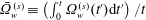 $\bar{\unicode[STIX]{x1D6FA}}_{w}^{(s)}\equiv \left(\int _{0}^{t}\unicode[STIX]{x1D6FA}_{w}^{(s)}(t^{\prime })\text{d}t^{\prime }\right)/t$
. Within this model, it is difficult to see how a singular current density can be created. Although
$\bar{\unicode[STIX]{x1D6FA}}_{w}^{(s)}\equiv \left(\int _{0}^{t}\unicode[STIX]{x1D6FA}_{w}^{(s)}(t^{\prime })\text{d}t^{\prime }\right)/t$
. Within this model, it is difficult to see how a singular current density can be created. Although
 $K$
characteristically increases linearly in time, the exponentiation in distance between trajectories
$K$
characteristically increases linearly in time, the exponentiation in distance between trajectories
 $\unicode[STIX]{x1D70E}$
can become large. Boozer (Reference Boozer2012) found that the maximum possible
$\unicode[STIX]{x1D70E}$
can become large. Boozer (Reference Boozer2012) found that the maximum possible
 $\unicode[STIX]{x1D70E}$
is proportional to
$\unicode[STIX]{x1D70E}$
is proportional to
 $K$
. The characteristic increase in the exponentiation
$K$
. The characteristic increase in the exponentiation
 $\unicode[STIX]{x1D70E}$
is linear in time in an ideal evolution.
$\unicode[STIX]{x1D70E}$
is linear in time in an ideal evolution.
A singular parallel current, called a sheet or delta-function current, can occur in an ideal evolution on the rational surfaces of topologically toroidal plasmas (Boozer & Pomphrey Reference Boozer and Pomphrey2010). These surfaces on which the magnetic field lines close on themselves are spatially isolated. It is difficult to imagine an analogue of a surface of perfectly closed field lines in a naturally occurring magnetic field.
The role of current sheets in fast magnetic reconnection has limitations related to magnetic field nulls. Both are difficult to produce, both are spatially isolated and neither is required in order to obtain reconnection at an Alfvénic speed.
2.5 Initiation of reconnection
When a magnetic evolution can be accurately approximated as ideal, both the sensitivity to the breaking of the ideal constraints and the magnitude of the breaking increase exponentially until a fast reconnection occurs. The time required to initiate a fast reconnection is called the trigger time.
Once the fast reconnection starts, the system is taken out of static force balance, and inertial or viscous forces are required. When force balance is maintained by inertia, the relaxation is by Alfvén waves. The relaxation can be complicated since the exponentiation
 $\unicode[STIX]{x1D70E}$
can change over the entire system during a relaxation, whichever is dominant inertia or viscosity. The relaxation can be studied in a simplified model such as that of § 3.
$\unicode[STIX]{x1D70E}$
can change over the entire system during a relaxation, whichever is dominant inertia or viscosity. The relaxation can be studied in a simplified model such as that of § 3.
3 Simple reconnection model
3.1 Model definition
Features of reconnection that arise in magnetic field structures that depend on all three spatial coordinates can be studied in highly simplified models since many features are generic. A model will be developed based on reduced magnetohydrodynamics (MHD) (Kadomtsev & Pogutse Reference Kadomtsev and Pogutse1974; Strauss Reference Strauss1976) in which the magnetic field has the form (van Ballegooijen Reference van Ballegooijen1985; Ng, Lin & Bhattacharjee Reference Ng, Lin and Bhattacharjee2012)
 $$\begin{eqnarray}\boldsymbol{B}=B_{g}(\hat{z}+\unicode[STIX]{x1D735}_{\bot }H\times \hat{z})\end{eqnarray}$$
in Cartesian coordinates, where
 $B_{g}$
is a constant guide field and
$B_{g}$
is a constant guide field and
 $\unicode[STIX]{x1D735}_{\bot }=\hat{x}\unicode[STIX]{x2202}/\unicode[STIX]{x2202}x+{\hat{y}}\unicode[STIX]{x2202}/\unicode[STIX]{x2202}y$
.
$\unicode[STIX]{x1D735}_{\bot }=\hat{x}\unicode[STIX]{x2202}/\unicode[STIX]{x2202}x+{\hat{y}}\unicode[STIX]{x2202}/\unicode[STIX]{x2202}y$
.
Van Ballegooijen used the magnetic field of (3.1) to study whether current singularities would develop but did not directly study magnetic reconnection.
The model system extends from a wall at
 $z=0$
to a wall at
$z=0$
to a wall at
 $z=L$
with
$z=L$
with
 $L|\unicode[STIX]{x1D735}_{\bot }H|$
remaining finite as
$L|\unicode[STIX]{x1D735}_{\bot }H|$
remaining finite as
 $L\rightarrow \infty$
. The
$L\rightarrow \infty$
. The
 $z=0$
wall is a rigid perfect conductor, but the
$z=0$
wall is a rigid perfect conductor, but the
 $z=L$
wall is a flowing perfect conductor that has a velocity
$z=L$
wall is a flowing perfect conductor that has a velocity
 $\boldsymbol{v}_{w}=\unicode[STIX]{x1D735}_{\bot }\unicode[STIX]{x1D719}_{w}\times \hat{z}$
. The guide field
$\boldsymbol{v}_{w}=\unicode[STIX]{x1D735}_{\bot }\unicode[STIX]{x1D719}_{w}\times \hat{z}$
. The guide field
 $B_{g}$
is too strong to be compressed, so the velocity of the plasma that lies in the region
$B_{g}$
is too strong to be compressed, so the velocity of the plasma that lies in the region
 $0<z<L$
can be assumed to have the velocity
$0<z<L$
can be assumed to have the velocity
 $$\begin{eqnarray}\boldsymbol{v}=\unicode[STIX]{x1D735}_{\bot }\unicode[STIX]{x1D719}\times \hat{z},\end{eqnarray}$$
where
 $\unicode[STIX]{x1D719}(x,y,z=L,t)=\unicode[STIX]{x1D719}_{w}(x,y,t)$
, which is the streamfunction in the flowing wall. Energy is put into the system by the moving wall and in steady state must be removed by dissipation.
$\unicode[STIX]{x1D719}(x,y,z=L,t)=\unicode[STIX]{x1D719}_{w}(x,y,t)$
, which is the streamfunction in the flowing wall. Energy is put into the system by the moving wall and in steady state must be removed by dissipation.
In addition to
 $B_{g}H$
being the
$B_{g}H$
being the
 $\hat{z}$
component of the vector potential,
$\hat{z}$
component of the vector potential,
 $H(x,y,z,t)$
is the Hamiltonian for the magnetic field lines with
$H(x,y,z,t)$
is the Hamiltonian for the magnetic field lines with
 $t$
a parameter,
$t$
a parameter,
 $$\begin{eqnarray}\displaystyle \frac{\text{d}x}{\text{d}z} & = & \displaystyle \frac{\unicode[STIX]{x2202}H}{\unicode[STIX]{x2202}y}\end{eqnarray}$$
 $$\begin{eqnarray}\displaystyle \frac{\text{d}y}{\text{d}z} & = & \displaystyle -\frac{\unicode[STIX]{x2202}H}{\unicode[STIX]{x2202}x}.\end{eqnarray}$$
Magnetic field line trajectories are given by a Hamiltonian of the same type as
 $H(x,y,z,t)$
in far more general representations of the magnetic field than that of (3.1). The magnetic field in a stellarator or tokamak can always be represented as (Boozer Reference Boozer1983, Reference Boozer2015)
$H(x,y,z,t)$
in far more general representations of the magnetic field than that of (3.1). The magnetic field in a stellarator or tokamak can always be represented as (Boozer Reference Boozer1983, Reference Boozer2015)
 $$\begin{eqnarray}2\unicode[STIX]{x03C0}\boldsymbol{B}=\unicode[STIX]{x1D735}\unicode[STIX]{x1D713}_{t}\times \unicode[STIX]{x1D735}\unicode[STIX]{x1D703}+\unicode[STIX]{x1D735}\unicode[STIX]{x1D711}\times \unicode[STIX]{x1D735}\unicode[STIX]{x1D713}_{p}(\unicode[STIX]{x1D713}_{t},\unicode[STIX]{x1D703},\unicode[STIX]{x1D711},t),\end{eqnarray}$$
where the poloidal flux
 $\unicode[STIX]{x1D713}_{p}$
is the field line Hamiltonian:
$\unicode[STIX]{x1D713}_{p}$
is the field line Hamiltonian:
 $\text{d}\unicode[STIX]{x1D703}/\text{d}\unicode[STIX]{x1D711}=\unicode[STIX]{x2202}\unicode[STIX]{x1D713}_{p}/\unicode[STIX]{x2202}\unicode[STIX]{x1D713}_{t}$
and
$\text{d}\unicode[STIX]{x1D703}/\text{d}\unicode[STIX]{x1D711}=\unicode[STIX]{x2202}\unicode[STIX]{x1D713}_{p}/\unicode[STIX]{x2202}\unicode[STIX]{x1D713}_{t}$
and
 $\text{d}\unicode[STIX]{x1D713}_{t}/\text{d}\unicode[STIX]{x1D711}=-\unicode[STIX]{x2202}\unicode[STIX]{x1D713}_{p}/\unicode[STIX]{x2202}\unicode[STIX]{x1D703}$
. The toroidal magnetic flux is
$\text{d}\unicode[STIX]{x1D713}_{t}/\text{d}\unicode[STIX]{x1D711}=-\unicode[STIX]{x2202}\unicode[STIX]{x1D713}_{p}/\unicode[STIX]{x2202}\unicode[STIX]{x1D703}$
. The toroidal magnetic flux is
 $\unicode[STIX]{x1D713}_{t}$
, the poloidal angle is
$\unicode[STIX]{x1D713}_{t}$
, the poloidal angle is
 $\unicode[STIX]{x1D703}$
and the toroidal angle is
$\unicode[STIX]{x1D703}$
and the toroidal angle is
 $\unicode[STIX]{x1D711}$
.
$\unicode[STIX]{x1D711}$
.
The streamfunction
 $\unicode[STIX]{x1D719}(x,y,z,t)$
is the Hamiltonian that describes the motion of plasma points in a constant-
$\unicode[STIX]{x1D719}(x,y,z,t)$
is the Hamiltonian that describes the motion of plasma points in a constant-
 $z$
plane,
$z$
plane,
 $$\begin{eqnarray}\displaystyle \frac{\text{d}x}{\text{d}t} & = & \displaystyle \frac{\unicode[STIX]{x2202}\unicode[STIX]{x1D719}}{\unicode[STIX]{x2202}y}\end{eqnarray}$$
 $$\begin{eqnarray}\displaystyle \frac{\text{d}y}{\text{d}t} & = & \displaystyle -\frac{\unicode[STIX]{x2202}\unicode[STIX]{x1D719}}{\unicode[STIX]{x2202}x}.\end{eqnarray}$$
That is,
 $z$
is a parameter in the Hamiltonian
$z$
is a parameter in the Hamiltonian
 $\unicode[STIX]{x1D719}(x,y,z,t)$
and not one of the canonical variables.
$\unicode[STIX]{x1D719}(x,y,z,t)$
and not one of the canonical variables.
3.2 Dimensionality and exponentiation
The fundamental difference in magnetic reconnection in two- versus three-coordinate systems is contained in the Hamiltonian description of magnetic field line trajectories. At each point in time, the Hamiltonian for magnetic field line trajectories, equations (3.3) and (3.4), depends on the same number of coordinates as the magnetic field. In the literature, a Hamiltonian
 $H(x,y)$
is said to be a one-degree-of-freedom Hamiltonian. A Hamiltonian
$H(x,y)$
is said to be a one-degree-of-freedom Hamiltonian. A Hamiltonian
 $H(x,y,z)$
is said to be a one-and-a-half-degree-of-freedom Hamiltonian. The qualitative differences between the trajectories given by these two types of Hamiltonians was so exciting to Lighthill (Reference Lighthill1986) that he titled an article in the Proceedings of the Royal Society ‘The Recently Recognized Failure of Predictability in Newtonian Dynamics’.
$H(x,y,z)$
is said to be a one-and-a-half-degree-of-freedom Hamiltonian. The qualitative differences between the trajectories given by these two types of Hamiltonians was so exciting to Lighthill (Reference Lighthill1986) that he titled an article in the Proceedings of the Royal Society ‘The Recently Recognized Failure of Predictability in Newtonian Dynamics’.
3.2.1 Two-coordinate Hamiltonians
When the magnetic field line Hamiltonian has the form
 $H(x,y)$
at a given point in time, equation (3.1) implies
$H(x,y)$
at a given point in time, equation (3.1) implies
 $H$
is constant along the magnetic field lines,
$H$
is constant along the magnetic field lines,
 $\boldsymbol{B}\boldsymbol{\cdot }\unicode[STIX]{x1D735}H=0$
. Neighbouring trajectories can separate as
$\boldsymbol{B}\boldsymbol{\cdot }\unicode[STIX]{x1D735}H=0$
. Neighbouring trajectories can separate as
 $e^{\unicode[STIX]{x1D70E}}$
for a Hamiltonian
$e^{\unicode[STIX]{x1D70E}}$
for a Hamiltonian
 $H(x,y)$
but only in an
$H(x,y)$
but only in an
 ${\approx}e^{-2\unicode[STIX]{x1D70E}}$
fraction of the area of the
${\approx}e^{-2\unicode[STIX]{x1D70E}}$
fraction of the area of the
 $(x,y)$
plane.
$(x,y)$
plane.
The only places at which magnetic field lines can exponentiate apart are at saddle points, where
 $H(x,y)$
has the Taylor expansion
$H(x,y)$
has the Taylor expansion
 $H=H_{sp}+(\unicode[STIX]{x2202}^{2}H/\unicode[STIX]{x2202}x\unicode[STIX]{x2202}y)_{sp}(x-x_{sp})(y-y_{sp})+\cdots$
. When
$H=H_{sp}+(\unicode[STIX]{x2202}^{2}H/\unicode[STIX]{x2202}x\unicode[STIX]{x2202}y)_{sp}(x-x_{sp})(y-y_{sp})+\cdots$
. When
 $a_{c}$
is the characteristic spatial scale of the function
$a_{c}$
is the characteristic spatial scale of the function
 $H(x,y)$
. Lines started within a radius
$H(x,y)$
. Lines started within a radius
 $a_{c}e^{-\unicode[STIX]{x1D70E}}$
of the point
$a_{c}e^{-\unicode[STIX]{x1D70E}}$
of the point
 $(x_{sp},y_{sp})$
can exponentiate
$(x_{sp},y_{sp})$
can exponentiate
 $\unicode[STIX]{x1D70E}$
times before being too far from the saddle point to be influenced by it. The fraction of the area in the
$\unicode[STIX]{x1D70E}$
times before being too far from the saddle point to be influenced by it. The fraction of the area in the
 $(x,y)$
plane in which
$(x,y)$
plane in which
 $\unicode[STIX]{x1D70E}$
exponentiations can take place is therefore
$\unicode[STIX]{x1D70E}$
exponentiations can take place is therefore
 ${\approx}e^{-2\unicode[STIX]{x1D70E}}$
.
${\approx}e^{-2\unicode[STIX]{x1D70E}}$
.
3.2.2 Three-coordinate Hamiltonians
As will be shown, when the magnetic field line Hamiltonian has the form
 $H(x,y,z)$
at a given point in time, the fraction of the area in a constant-
$H(x,y,z)$
at a given point in time, the fraction of the area in a constant-
 $z$
plane occupied by lines that exponentiate apart is generically of order unity.
$z$
plane occupied by lines that exponentiate apart is generically of order unity.
The trajectory of a magnetic field line can be written as
 $\boldsymbol{x}(x_{s},y_{s},\ell )$
, where
$\boldsymbol{x}(x_{s},y_{s},\ell )$
, where
 $(x_{s},y_{s})$
is the starting point of the trajectory. The distance along the line is
$(x_{s},y_{s})$
is the starting point of the trajectory. The distance along the line is
 $\ell$
, which in the reduced MHD model is indistinguishable from
$\ell$
, which in the reduced MHD model is indistinguishable from
 $z$
. That is,
$z$
. That is,
 $$\begin{eqnarray}\displaystyle & \displaystyle \boldsymbol{x}(x_{s},y_{s},\ell )=\boldsymbol{x}_{\bot }(x_{s},y_{s},\ell )+\ell \hat{z}, & \displaystyle\end{eqnarray}$$
 $$\begin{eqnarray}\displaystyle & \text{where}\quad \displaystyle \boldsymbol{x}_{\bot }(x_{s},y_{s},\ell )\equiv x(x_{s},y_{s},\ell )\hat{x}+y(x_{s},y_{s},\ell ){\hat{y}}, & \displaystyle\end{eqnarray}$$
 $$\begin{eqnarray}\displaystyle & \displaystyle x(x_{s},y_{s},\ell =0)=x_{s},\quad \text{and}\quad y(x_{s},y_{s},\ell =0)=y_{s}. & \displaystyle\end{eqnarray}$$
It is convenient to use
 $\ell$
to indicate the use of
$\ell$
to indicate the use of
 $(x_{s},y_{s},\ell )$
as spatial coordinates rather than Cartesian coordinates
$(x_{s},y_{s},\ell )$
as spatial coordinates rather than Cartesian coordinates
 $(x,y,z)$
. The position vector
$(x,y,z)$
. The position vector
 $\boldsymbol{x}(x_{s},y_{s},\ell )$
defines a coordinate system in which the magnetic field lines are trivial.
$\boldsymbol{x}(x_{s},y_{s},\ell )$
defines a coordinate system in which the magnetic field lines are trivial.
Three notations can be used for the derivative of a function along a magnetic field line:
 $$\begin{eqnarray}\displaystyle \left(\frac{\unicode[STIX]{x2202}f}{\unicode[STIX]{x2202}z}\right)_{x_{s}y_{s}}=\frac{\text{d}f}{\text{d}z}=\frac{\unicode[STIX]{x2202}f}{\unicode[STIX]{x2202}\ell }=\frac{\text{d}f}{\text{d}\ell }. & & \displaystyle\end{eqnarray}$$
The total derivative of a function with respect to
 $z$
means along a magnetic field line as does either the partial or the total derivative with respect to
$z$
means along a magnetic field line as does either the partial or the total derivative with respect to
 $\ell$
.
$\ell$
.
The separation between neighbouring trajectories is
 $$\begin{eqnarray}\displaystyle & \displaystyle \unicode[STIX]{x1D739}_{\bot }\equiv \frac{\unicode[STIX]{x2202}\boldsymbol{x}_{\bot }}{\unicode[STIX]{x2202}x_{s}}\unicode[STIX]{x1D6FF}x_{s}+\frac{\unicode[STIX]{x2202}\boldsymbol{x}_{\bot }}{\unicode[STIX]{x2202}y_{s}}\unicode[STIX]{x1D6FF}y_{s}, & \displaystyle\end{eqnarray}$$
 $$\begin{eqnarray}\displaystyle & \text{so}\quad \displaystyle \left(\begin{array}{@{}c@{}}\unicode[STIX]{x1D6FF}_{x}\\ \unicode[STIX]{x1D6FF}_{y}\end{array}\right)=\left(\begin{array}{@{}cc@{}}\displaystyle \frac{\unicode[STIX]{x2202}x}{\unicode[STIX]{x2202}x_{s}} & \displaystyle \frac{\unicode[STIX]{x2202}x}{\unicode[STIX]{x2202}y_{s}}\\ \displaystyle \frac{\unicode[STIX]{x2202}y}{\unicode[STIX]{x2202}x_{s}} & \displaystyle \frac{\unicode[STIX]{x2202}y}{\unicode[STIX]{x2202}y_{s}}\end{array}\right)\left(\begin{array}{@{}c@{}}\unicode[STIX]{x1D6FF}x_{s}\\ \unicode[STIX]{x1D6FF}y_{s}\end{array}\right), & \displaystyle\end{eqnarray}$$
where
 $\unicode[STIX]{x1D739}_{\bot }=\unicode[STIX]{x1D6FF}_{x}\hat{x}+\unicode[STIX]{x1D6FF}_{y}{\hat{y}}$
. The Jacobian matrix of
$\unicode[STIX]{x1D739}_{\bot }=\unicode[STIX]{x1D6FF}_{x}\hat{x}+\unicode[STIX]{x1D6FF}_{y}{\hat{y}}$
. The Jacobian matrix of
 $\boldsymbol{x}_{\bot }(x_{s},y_{s},\ell )$
is
$\boldsymbol{x}_{\bot }(x_{s},y_{s},\ell )$
is
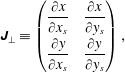 $$\begin{eqnarray}\unicode[STIX]{x1D645}_{\bot }\equiv \left(\begin{array}{@{}cc@{}}\displaystyle \frac{\unicode[STIX]{x2202}x}{\unicode[STIX]{x2202}x_{s}} & \displaystyle \frac{\unicode[STIX]{x2202}x}{\unicode[STIX]{x2202}y_{s}}\\ \displaystyle \frac{\unicode[STIX]{x2202}y}{\unicode[STIX]{x2202}x_{s}} & \displaystyle \frac{\unicode[STIX]{x2202}y}{\unicode[STIX]{x2202}y_{s}}\end{array}\right),\end{eqnarray}$$
and the determinant of the Jacobian matrix is the Jacobian
 ${\mathcal{J}}_{\bot }$
of the
${\mathcal{J}}_{\bot }$
of the
 $(x_{s},y_{s})$
coordinates. Since the area element in the
$(x_{s},y_{s})$
coordinates. Since the area element in the
 $\hat{z}$
direction is
$\hat{z}$
direction is
 $\text{d}\boldsymbol{a}=\hat{z}{\mathcal{J}}_{\bot }\text{d}x_{s}\text{d}y_{s}$
, magnetic flux conservation implies
$\text{d}\boldsymbol{a}=\hat{z}{\mathcal{J}}_{\bot }\text{d}x_{s}\text{d}y_{s}$
, magnetic flux conservation implies
 ${\mathcal{J}}_{\bot }=1$
. The mathematical implication of a unit Jacobian is that the singular value decomposition of the Jacobian matrix has the form
${\mathcal{J}}_{\bot }=1$
. The mathematical implication of a unit Jacobian is that the singular value decomposition of the Jacobian matrix has the form
 $$\begin{eqnarray}\unicode[STIX]{x1D645}_{\bot }(x_{s},y_{s},\ell )=\unicode[STIX]{x1D650}_{\bot }\boldsymbol{\cdot }\left(\begin{array}{@{}cc@{}}e^{\unicode[STIX]{x1D70E}_{\bot }} & 0\\ 0 & e^{-\unicode[STIX]{x1D70E}_{\bot }}\end{array}\right)\boldsymbol{\cdot }\unicode[STIX]{x1D651}_{\bot }^{\dagger },\end{eqnarray}$$
where
 $\unicode[STIX]{x1D650}_{\bot }$
and
$\unicode[STIX]{x1D650}_{\bot }$
and
 $\unicode[STIX]{x1D651}_{\bot }$
are orthogonal matrices. There is a direction in which the magnetic field lines approach each other exponentially, but when integrating lines, numerical errors will quickly cause the exponential separation to overwhelm the exponential convergence.
$\unicode[STIX]{x1D651}_{\bot }$
are orthogonal matrices. There is a direction in which the magnetic field lines approach each other exponentially, but when integrating lines, numerical errors will quickly cause the exponential separation to overwhelm the exponential convergence.
The distance squared between neighbouring magnetic field lines is
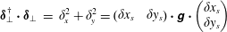 $$\begin{eqnarray}\displaystyle \unicode[STIX]{x1D739}_{\bot }^{\dagger }\boldsymbol{\cdot }\unicode[STIX]{x1D739}_{\bot } & = & \displaystyle \unicode[STIX]{x1D6FF}_{x}^{2}+\unicode[STIX]{x1D6FF}_{y}^{2}=(\begin{array}{@{}cc@{}}\unicode[STIX]{x1D6FF}x_{s} & \unicode[STIX]{x1D6FF}y_{s}\end{array})\boldsymbol{\cdot }\unicode[STIX]{x1D65C}\boldsymbol{\cdot }\left(\begin{array}{@{}c@{}}\unicode[STIX]{x1D6FF}x_{s}\\ \unicode[STIX]{x1D6FF}y_{s}\end{array}\right)\end{eqnarray}$$
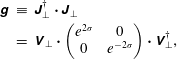 $$\begin{eqnarray}\displaystyle \displaystyle \unicode[STIX]{x1D65C} & \equiv & \displaystyle \unicode[STIX]{x1D645}_{\bot }^{\dagger }\boldsymbol{\cdot }\unicode[STIX]{x1D645}_{\bot }\nonumber\\ \displaystyle & = & \displaystyle \unicode[STIX]{x1D651}_{\bot }\boldsymbol{\cdot }\left(\begin{array}{@{}cc@{}}e^{2\unicode[STIX]{x1D70E}} & 0\\ 0 & e^{-2\unicode[STIX]{x1D70E}}\end{array}\right)\boldsymbol{\cdot }\unicode[STIX]{x1D651}_{\bot }^{\dagger },\end{eqnarray}$$
where
 $\unicode[STIX]{x1D65C}$
is the metric tensor.
$\unicode[STIX]{x1D65C}$
is the metric tensor.
Equations (3.16) and (3.17) demonstrate that neighbouring magnetic field lines have a separation that depends exponentially on
 $\unicode[STIX]{x1D70E}_{\bot }(x_{s},y_{s},\ell )$
. Neighbouring magnetic fields lines characteristically exponentiate apart with the distance
$\unicode[STIX]{x1D70E}_{\bot }(x_{s},y_{s},\ell )$
. Neighbouring magnetic fields lines characteristically exponentiate apart with the distance
 $\ell$
along a line unless there is a constraint that prevents the exponentiation, as when the magnetic field depends on only two spatial coordinates.
$\ell$
along a line unless there is a constraint that prevents the exponentiation, as when the magnetic field depends on only two spatial coordinates.
Section 2.2 studied the exponentially increasing separation of streamlines
 $\boldsymbol{x}(\boldsymbol{x}_{0},t)$
of the magnetic field line velocity. In the reduced MHD model being considered here, the Jacobian of the streamlines is unity, and the Lyapunov exponents of the streamlines stated as
$\boldsymbol{x}(\boldsymbol{x}_{0},t)$
of the magnetic field line velocity. In the reduced MHD model being considered here, the Jacobian of the streamlines is unity, and the Lyapunov exponents of the streamlines stated as
 $\unicode[STIX]{x1D70E}(\ell ,t)$
and the
$\unicode[STIX]{x1D70E}(\ell ,t)$
and the
 $\unicode[STIX]{x1D70E}_{\bot }$
of the field lines at a given time can and will be identified.
$\unicode[STIX]{x1D70E}_{\bot }$
of the field lines at a given time can and will be identified.
3.3 Magnetic field evolution
The evolution equations for a magnetic field have two parts: (i) the evolution equations for
 $\boldsymbol{B}$
when the plasma flow velocity
$\boldsymbol{B}$
when the plasma flow velocity
 $\boldsymbol{v}$
is known and (ii) the evolution equation for the plasma velocity, which will be obtained from force balance in the next section. This section will assume
$\boldsymbol{v}$
is known and (ii) the evolution equation for the plasma velocity, which will be obtained from force balance in the next section. This section will assume
 $\boldsymbol{v}$
is known and derive four equations: (i) equation (3.23) relating the time derivative of the Hamiltonian to the streamfunction of the flow, (ii) equation (3.24) relating the Hamiltonian
$\boldsymbol{v}$
is known and derive four equations: (i) equation (3.23) relating the time derivative of the Hamiltonian to the streamfunction of the flow, (ii) equation (3.24) relating the Hamiltonian
 $H$
to the parallel-current function
$H$
to the parallel-current function
 $K\equiv \unicode[STIX]{x1D707}_{0}j_{||}/B$
, (iii) equation (3.26) relating the streamfunction of the flow
$K\equiv \unicode[STIX]{x1D707}_{0}j_{||}/B$
, (iii) equation (3.26) relating the streamfunction of the flow
 $\unicode[STIX]{x1D719}$
to the flow vorticity
$\unicode[STIX]{x1D719}$
to the flow vorticity
 $\unicode[STIX]{x1D6FA}$
and (iv) equation (3.27) relating the time derivative of
$\unicode[STIX]{x1D6FA}$
and (iv) equation (3.27) relating the time derivative of
 $K$
moving with the flow to the derivative of the vorticity
$K$
moving with the flow to the derivative of the vorticity
 $\unicode[STIX]{x1D6FA}$
along a field line.
$\unicode[STIX]{x1D6FA}$
along a field line.
3.3.1 Relation between
$\unicode[STIX]{x2202}H/\unicode[STIX]{x2202}t$
and
$\text{d}\unicode[STIX]{x1D719}/\text{d}\ell$


The time derivative of the magnetic field line Hamiltonian is related to the streamfunction of the flow
 $\unicode[STIX]{x1D719}$
by Ohm’s law and Faraday’s law.
$\unicode[STIX]{x1D719}$
by Ohm’s law and Faraday’s law.
The electric field is given by Ohm’s law, which will be written as
 $$\begin{eqnarray}\displaystyle \boldsymbol{E}+\boldsymbol{v}\times \boldsymbol{B} & = & \displaystyle {\mathcal{N}}_{B}B_{g}\hat{z},\end{eqnarray}$$
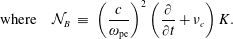 $$\begin{eqnarray}\displaystyle \text{where}\quad {\mathcal{N}}_{B} & \equiv & \displaystyle \left(\frac{c}{\unicode[STIX]{x1D714}_{\text{pe}}}\right)^{2}\left(\frac{\unicode[STIX]{x2202}}{\unicode[STIX]{x2202}t}+\unicode[STIX]{x1D708}_{c}\right)K.\end{eqnarray}$$
 ${\mathcal{N}}_{B}$
represents the non-ideal effects in Ohm’s law and hence in the magnetic evolution. The resistivity
${\mathcal{N}}_{B}$
represents the non-ideal effects in Ohm’s law and hence in the magnetic evolution. The resistivity
 $\unicode[STIX]{x1D702}$
is related to the electron collision frequency
$\unicode[STIX]{x1D702}$
is related to the electron collision frequency
 $\unicode[STIX]{x1D708}_{c}$
by
$\unicode[STIX]{x1D708}_{c}$
by
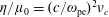 $\unicode[STIX]{x1D702}/\unicode[STIX]{x1D707}_{0}=(c/\unicode[STIX]{x1D714}_{\text{pe}})^{2}\unicode[STIX]{x1D708}_{c}$
. The term involving the time derivative of the parallel-current density, where
$\unicode[STIX]{x1D702}/\unicode[STIX]{x1D707}_{0}=(c/\unicode[STIX]{x1D714}_{\text{pe}})^{2}\unicode[STIX]{x1D708}_{c}$
. The term involving the time derivative of the parallel-current density, where
 $K\equiv \unicode[STIX]{x1D707}_{0}j_{||}/B_{g}$
, is due to the electron inertia and is always present since the electron is the lightest charged particle.
$K\equiv \unicode[STIX]{x1D707}_{0}j_{||}/B_{g}$
, is due to the electron inertia and is always present since the electron is the lightest charged particle.
Faraday’s law implies
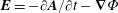 $\boldsymbol{E}=-\unicode[STIX]{x2202}\boldsymbol{A}/\unicode[STIX]{x2202}t-\unicode[STIX]{x1D735}\unicode[STIX]{x1D6F7}$
, where the potential
$\boldsymbol{E}=-\unicode[STIX]{x2202}\boldsymbol{A}/\unicode[STIX]{x2202}t-\unicode[STIX]{x1D735}\unicode[STIX]{x1D6F7}$
, where the potential
 $\unicode[STIX]{x1D6F7}$
depends on the gauge used to represent the vector potential. When the velocity
$\unicode[STIX]{x1D6F7}$
depends on the gauge used to represent the vector potential. When the velocity
 $\boldsymbol{v}=\unicode[STIX]{x1D735}\unicode[STIX]{x1D719}\times \hat{z}$
, equation (3.2), the clever choice of gauge gives
$\boldsymbol{v}=\unicode[STIX]{x1D735}\unicode[STIX]{x1D719}\times \hat{z}$
, equation (3.2), the clever choice of gauge gives
 $$\begin{eqnarray}\boldsymbol{E}=\left(-\frac{\unicode[STIX]{x2202}H}{\unicode[STIX]{x2202}t}\hat{z}+\unicode[STIX]{x1D735}\unicode[STIX]{x1D719}\right)B_{g}.\end{eqnarray}$$
Ohm’s law implies, using
 $$\begin{eqnarray}\displaystyle \boldsymbol{v}\times \boldsymbol{B} & = & \displaystyle (\unicode[STIX]{x1D735}\unicode[STIX]{x1D719}\times \hat{z})\times \boldsymbol{B}\end{eqnarray}$$
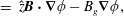 $$\begin{eqnarray}\displaystyle & = & \displaystyle \hat{z}\boldsymbol{B}\boldsymbol{\cdot }\unicode[STIX]{x1D735}\unicode[STIX]{x1D719}-B_{g}\unicode[STIX]{x1D735}\unicode[STIX]{x1D719},\end{eqnarray}$$
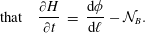 $$\begin{eqnarray}\displaystyle \text{that}\quad \frac{\unicode[STIX]{x2202}H}{\unicode[STIX]{x2202}t} & = & \displaystyle \frac{\text{d}\unicode[STIX]{x1D719}}{\text{d}\ell }-{\mathcal{N}}_{B}.\end{eqnarray}$$
3.3.2 Relation between
$H$
and
$K$


The relation between the Hamiltonian and the parallel-current function follows simply from Ampere’s law,
 $\unicode[STIX]{x1D735}\times \boldsymbol{B}=\unicode[STIX]{x1D707}_{0}\,\boldsymbol{j}$
,
$\unicode[STIX]{x1D735}\times \boldsymbol{B}=\unicode[STIX]{x1D707}_{0}\,\boldsymbol{j}$
,
 $$\begin{eqnarray}\unicode[STIX]{x1D6FB}_{\bot }^{2}H=-K.\end{eqnarray}$$
3.3.3 Relation between
$\unicode[STIX]{x1D719}$
and
$\unicode[STIX]{x1D6FA}$


The vorticity of the flow is
 $$\begin{eqnarray}\displaystyle \unicode[STIX]{x1D6FA} & \equiv & \displaystyle \hat{z}\boldsymbol{\cdot }\unicode[STIX]{x1D735}\times \boldsymbol{v}\end{eqnarray}$$
 $$\begin{eqnarray}\displaystyle & = & \displaystyle -\unicode[STIX]{x1D6FB}_{\bot }^{2}\unicode[STIX]{x1D719},\end{eqnarray}$$
where
 $\unicode[STIX]{x1D719}$
is the streamfunction.
$\unicode[STIX]{x1D719}$
is the streamfunction.
3.3.4 Relation between
$\text{d}K/\text{d}t$
and
$\text{d}\unicode[STIX]{x1D6FA}/\text{d}\ell$


Two equations from the appendix, equations (D 1) relating the total time derivative to the velocity potential and (D 4) for the commutator of
 $\text{d}/\text{d}t$
and
$\text{d}/\text{d}t$
and
 $\text{d}/\text{d}\ell$
, then imply
$\text{d}/\text{d}\ell$
, then imply
 $$\begin{eqnarray}\frac{\text{d}K}{\text{d}t}=\frac{\text{d}\unicode[STIX]{x1D6FA}}{\text{d}\ell }+\unicode[STIX]{x1D6FB}_{\bot }^{2}{\mathcal{N}}_{B}.\end{eqnarray}$$
The dissipative term
 $\unicode[STIX]{x1D6FB}_{\bot }^{2}{\mathcal{N}}_{B}$
acts to flatten
$\unicode[STIX]{x1D6FB}_{\bot }^{2}{\mathcal{N}}_{B}$
acts to flatten
 $K$
across the magnetic field lines.
$K$
across the magnetic field lines.
In an ideal magnetic evolution,
 ${\mathcal{N}}_{B}=0$
and
${\mathcal{N}}_{B}=0$
and
 $\boldsymbol{v}$
is the velocity of the magnetic field lines. The twisting of the field lines around themselves, given by
$\boldsymbol{v}$
is the velocity of the magnetic field lines. The twisting of the field lines around themselves, given by
 $\text{d}\unicode[STIX]{x1D6FA}/\text{d}\ell$
, gives the time rate of change of the current
$\text{d}\unicode[STIX]{x1D6FA}/\text{d}\ell$
, gives the time rate of change of the current
 $K$
required to be consistent with both Faraday’s and Ampere’s law.
$K$
required to be consistent with both Faraday’s and Ampere’s law.
3.3.5 Discussion of
$B$
evolution

The current function
 $K$
need not be become large to produce a fast magnetic reconnection. As the exponentiation
$K$
need not be become large to produce a fast magnetic reconnection. As the exponentiation
 $\unicode[STIX]{x1D70E}$
of neighbouring trajectories becomes larger,
$\unicode[STIX]{x1D70E}$
of neighbouring trajectories becomes larger,
 $K$
need only increase in proportion to
$K$
need only increase in proportion to
 $\unicode[STIX]{x1D70E}$
(Boozer Reference Boozer2012).
$\unicode[STIX]{x1D70E}$
(Boozer Reference Boozer2012).
The operator
 $\unicode[STIX]{x1D6FB}_{\bot }^{2}{\mathcal{N}}_{B}$
becomes very large when magnetic field lines exponentiate apart. The theory of general coordinates (see the appendix of Boozer Reference Boozer2004) implies
$\unicode[STIX]{x1D6FB}_{\bot }^{2}{\mathcal{N}}_{B}$
becomes very large when magnetic field lines exponentiate apart. The theory of general coordinates (see the appendix of Boozer Reference Boozer2004) implies
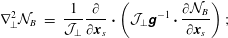 $$\begin{eqnarray}\displaystyle \unicode[STIX]{x1D6FB}_{\bot }^{2}{\mathcal{N}}_{B} & = & \displaystyle \frac{1}{{\mathcal{J}}_{\bot }}\frac{\unicode[STIX]{x2202}}{\unicode[STIX]{x2202}\boldsymbol{x}_{s}}\boldsymbol{\cdot }\left({\mathcal{J}}_{\bot }\unicode[STIX]{x1D65C}^{-1}\boldsymbol{\cdot }\frac{\unicode[STIX]{x2202}{\mathcal{N}}_{B}}{\unicode[STIX]{x2202}\boldsymbol{x}_{s}}\right);\end{eqnarray}$$
 $$\begin{eqnarray}\displaystyle \unicode[STIX]{x1D65C}^{-1} & = & \displaystyle \unicode[STIX]{x1D651}_{\bot }\boldsymbol{\cdot }\left(\begin{array}{@{}cc@{}}e^{-2\unicode[STIX]{x1D70E}} & 0\\ 0 & e^{2\unicode[STIX]{x1D70E}}\end{array}\right)\boldsymbol{\cdot }\unicode[STIX]{x1D651}_{\bot }^{\dagger }.\end{eqnarray}$$
Although the operator
 $\unicode[STIX]{x1D6FB}_{\bot }^{2}$
can be calculated in the field line coordinates
$\unicode[STIX]{x1D6FB}_{\bot }^{2}$
can be calculated in the field line coordinates
 $(x_{s},y_{s},\ell )$
, equation (3.28), this operator is easier to calculate and to invert in ordinary Cartesian coordinates
$(x_{s},y_{s},\ell )$
, equation (3.28), this operator is easier to calculate and to invert in ordinary Cartesian coordinates
 $(x,y,z)$
.
$(x,y,z)$
.
To determine the evolution of the magnetic field lines
 $\boldsymbol{x}_{\bot }(x_{s},y_{s},z,t)$
, the Hamiltonian
$\boldsymbol{x}_{\bot }(x_{s},y_{s},z,t)$
, the Hamiltonian
 $H(x,y,z,t)$
is required at each time
$H(x,y,z,t)$
is required at each time
 $t$
.
$t$
.
 $H(x,y,z,t)$
can be obtained from
$H(x,y,z,t)$
can be obtained from
 $K(x_{s},y_{s},z,t)$
by use of the Green’s function for a two-dimensional Laplacian:
$K(x_{s},y_{s},z,t)$
by use of the Green’s function for a two-dimensional Laplacian:
 $$\begin{eqnarray}\displaystyle H=\int K\frac{\ln \left((x-x^{\prime })^{2}+(y-y^{\prime })^{2}\right)}{4\unicode[STIX]{x03C0}}\,\text{d}x_{s}\,\text{d}y_{s}, & & \displaystyle\end{eqnarray}$$
where
 $K$
,
$K$
,
 $x^{\prime }$
, and
$x^{\prime }$
, and
 $y^{\prime }$
are written as functions of
$y^{\prime }$
are written as functions of
 $(x_{s},y_{s},z,t)$
. The Jacobian between
$(x_{s},y_{s},z,t)$
. The Jacobian between
 $(x_{s},y_{s})$
and
$(x_{s},y_{s})$
and
 $(x,y)$
coordinates is unity, so
$(x,y)$
coordinates is unity, so
 $\text{d}x^{\prime }\,\text{d}y^{\prime }=\text{d}x_{s}\,\text{d}y_{s}$
.
$\text{d}x^{\prime }\,\text{d}y^{\prime }=\text{d}x_{s}\,\text{d}y_{s}$
.
 $H(x,y,z,t)$
can also be obtained by Fourier decomposition:
$H(x,y,z,t)$
can also be obtained by Fourier decomposition:
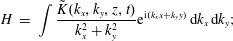 $$\begin{eqnarray}\displaystyle H & = & \displaystyle \int \frac{\tilde{K}(k_{x},k_{y},z,t)}{k_{x}^{2}+k_{y}^{2}}\text{e}^{\text{i}(k_{x}x+k_{y}y)}\,\text{d}k_{x}\,\text{d}k_{y};\end{eqnarray}$$
 $$\begin{eqnarray}\displaystyle \tilde{K} & = & \displaystyle \frac{1}{(2\unicode[STIX]{x03C0})^{2}}\int K\text{e}^{-\text{i}(k_{x}x+k_{y}y)}\,\text{d}x\,\text{d}y,\end{eqnarray}$$
 $$\begin{eqnarray}\displaystyle & = & \displaystyle \frac{1}{(2\unicode[STIX]{x03C0})^{2}}\int K\text{e}^{-\text{i}(k_{x}x+k_{y}y)}\,\text{d}x_{s}\,\text{d}y_{s},\end{eqnarray}$$
where
 $K$
,
$K$
,
 $x$
, and
$x$
, and
 $y$
in the last integral are written as functions of
$y$
in the last integral are written as functions of
 $(x_{s},y_{s},z,t)$
. A simple version of the reduced MHD model is periodic in the
$(x_{s},y_{s},z,t)$
. A simple version of the reduced MHD model is periodic in the
 $x$
and
$x$
and
 $y$
directions with a periodicity length
$y$
directions with a periodicity length
 $2\unicode[STIX]{x03C0}a$
, so
$2\unicode[STIX]{x03C0}a$
, so
 $k_{x}=m/(2\unicode[STIX]{x03C0}a)$
and
$k_{x}=m/(2\unicode[STIX]{x03C0}a)$
and
 $k_{y}=n/(2\unicode[STIX]{x03C0}a)$
with
$k_{y}=n/(2\unicode[STIX]{x03C0}a)$
with
 $m$
and
$m$
and
 $n$
integers.
$n$
integers.
Equation (3.31) implies the smallest wavenumbers
 $\boldsymbol{k}_{\bot }=k_{x}\hat{x}+k_{y}{\hat{y}}$
largely determine
$\boldsymbol{k}_{\bot }=k_{x}\hat{x}+k_{y}{\hat{y}}$
largely determine
 $H(x,y,z,t)$
. As discussed in § 2.1, the smallest wavenumber terms in
$H(x,y,z,t)$
. As discussed in § 2.1, the smallest wavenumber terms in
 $H$
produce the largest separations between magnetic field lines and, therefore, have the largest effect on magnetic reconnection. There is nothing in the model that rules out short wavelength turbulence. Indeed, wavelengths of order
$H$
produce the largest separations between magnetic field lines and, therefore, have the largest effect on magnetic reconnection. There is nothing in the model that rules out short wavelength turbulence. Indeed, wavelengths of order
 $a_{c}e^{-\unicode[STIX]{x1D70E}}$
are strongly driven, and their effect on reconnection is an important question.
$a_{c}e^{-\unicode[STIX]{x1D70E}}$
are strongly driven, and their effect on reconnection is an important question.
3.4 Force balance
General features of magnetic reconnection can be studied by considering the generic properties of a flow. This was done in §§ 1 and 2 and could be done using the equations derived in § 3.3. To actually know the flow and the evolution of the magnetic field, an additional equation is required, which is given by force balance. The required (3.40), which relates
 $\text{d}\unicode[STIX]{x1D6FA}/\text{d}t$
to
$\text{d}\unicode[STIX]{x1D6FA}/\text{d}t$
to
 $\text{d}K/\text{d}\ell$
will be derived in this section.
$\text{d}K/\text{d}\ell$
will be derived in this section.
The smallness of the Debye length implies the current must be divergence free (Boozer Reference Boozer2015). That and the expression for the electromagnetic or Lorentz force
 $\boldsymbol{f}=\boldsymbol{j}\times \boldsymbol{B}$
implies
$\boldsymbol{f}=\boldsymbol{j}\times \boldsymbol{B}$
implies
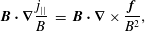 $$\begin{eqnarray}\displaystyle \boldsymbol{B}\boldsymbol{\cdot }\unicode[STIX]{x1D735}\frac{j_{||}}{B} & = & \displaystyle \boldsymbol{B}\boldsymbol{\cdot }\unicode[STIX]{x1D735}\times \frac{\boldsymbol{f}}{B^{2}},\end{eqnarray}$$
 $$\begin{eqnarray}\displaystyle \text{or}\quad \frac{\text{d}K}{\text{d}\ell } & = & \displaystyle \frac{1}{V_{A}^{2}}\hat{z}\boldsymbol{\cdot }\unicode[STIX]{x1D735}\times \frac{\boldsymbol{f}}{\unicode[STIX]{x1D70C}_{0}};\end{eqnarray}$$
 $$\begin{eqnarray}\displaystyle V_{A}^{2} & \equiv & \displaystyle \frac{B_{g}^{2}}{\unicode[STIX]{x1D707}_{0}\unicode[STIX]{x1D70C}_{0}},\end{eqnarray}$$
where
 $\unicode[STIX]{x1D70C}_{0}$
is the plasma density, which is assumed to be a constant, and
$\unicode[STIX]{x1D70C}_{0}$
is the plasma density, which is assumed to be a constant, and
 $V_{A}$
is the Alfvén velocity.
$V_{A}$
is the Alfvén velocity.
The force exerted by the plasma consists of inertial and viscosity terms,
 $$\begin{eqnarray}\displaystyle \frac{\boldsymbol{f}}{\unicode[STIX]{x1D70C}_{0}} & = & \displaystyle \frac{\unicode[STIX]{x2202}\boldsymbol{v}}{\unicode[STIX]{x2202}t}+\boldsymbol{v}\boldsymbol{\cdot }\unicode[STIX]{x1D735}\boldsymbol{v}-\unicode[STIX]{x1D708}_{v}\unicode[STIX]{x1D6FB}_{\bot }^{2}\boldsymbol{v},\end{eqnarray}$$
 $$\begin{eqnarray}\displaystyle \text{and}\quad \boldsymbol{v}\boldsymbol{\cdot }\unicode[STIX]{x1D735}\boldsymbol{v} & = & \displaystyle \unicode[STIX]{x1D735}(v^{2}/2)-\boldsymbol{v}\times \unicode[STIX]{x1D735}\times \boldsymbol{v},\end{eqnarray}$$
 $$\begin{eqnarray}\displaystyle \text{so}\quad \hat{z}\boldsymbol{\cdot }\unicode[STIX]{x1D735}\times \frac{\boldsymbol{f}}{\unicode[STIX]{x1D70C}_{0}} & = & \displaystyle \frac{\text{d}\unicode[STIX]{x1D6FA}}{\text{d}t}-\unicode[STIX]{x1D708}_{v}\unicode[STIX]{x1D6FB}_{\bot }^{2}\unicode[STIX]{x1D6FA}.\end{eqnarray}$$
Consequently, force balance implies
 $$\begin{eqnarray}\displaystyle \frac{\text{d}K}{\text{d}\ell } & = & \displaystyle \frac{1}{V_{A}^{2}}\left(\frac{\text{d}\unicode[STIX]{x1D6FA}}{\text{d}t}-{\mathcal{N}}_{v}\right),\end{eqnarray}$$
 $$\begin{eqnarray}\displaystyle \text{where}\quad {\mathcal{N}}_{v} & \equiv & \displaystyle \unicode[STIX]{x1D708}_{v}\unicode[STIX]{x1D6FB}_{\bot }^{2}\unicode[STIX]{x1D6FA}\end{eqnarray}$$
gives the non-ideality of the plasma flow.
3.5 Ideal evolution
The evolution in the absence of dissipation,
 ${\mathcal{N}}_{B}=0$
and
${\mathcal{N}}_{B}=0$
and
 ${\mathcal{N}}_{v}=0$
, is given by an Alfvén wave equation, equation (3.45). The ideal equations are
${\mathcal{N}}_{v}=0$
, is given by an Alfvén wave equation, equation (3.45). The ideal equations are
 $$\begin{eqnarray}\displaystyle \unicode[STIX]{x1D6FB}_{\bot }^{2}H & = & \displaystyle -K\end{eqnarray}$$
 $$\begin{eqnarray}\displaystyle \frac{\text{d}K}{\text{d}t} & = & \displaystyle \frac{\text{d}\unicode[STIX]{x1D6FA}}{\text{d}\ell }\end{eqnarray}$$
 $$\begin{eqnarray}\displaystyle \frac{\text{d}K}{\text{d}\ell } & = & \displaystyle \frac{1}{V_{A}^{2}}\frac{\text{d}\unicode[STIX]{x1D6FA}}{\text{d}t}.\end{eqnarray}$$
When the evolution is ideal,
 $\text{d}/\text{d}\ell$
and
$\text{d}/\text{d}\ell$
and
 $\text{d}/\text{d}t$
commute, see equation (D 8). In the ideal case, being fixed to a fluid point, as in a
$\text{d}/\text{d}t$
commute, see equation (D 8). In the ideal case, being fixed to a fluid point, as in a
 $\text{d}/\text{d}t$
derivative, or fixed on a magnetic field line, as in a
$\text{d}/\text{d}t$
derivative, or fixed on a magnetic field line, as in a
 $\text{d}/\text{d}\ell$
derivative, is the same. The implication is
$\text{d}/\text{d}\ell$
derivative, is the same. The implication is
 $$\begin{eqnarray}\frac{\text{d}^{2}\unicode[STIX]{x1D6FA}}{\text{d}t^{2}}=V_{A}^{2}\frac{\text{d}^{2}\unicode[STIX]{x1D6FA}}{\text{d}\ell ^{2}}.\end{eqnarray}$$
Equation (3.45) is an equation for Alfvén waves along a magnetic field line that is defined by its position
 $(x_{s},y_{s})$
at
$(x_{s},y_{s})$
at
 $\ell =0$
. Since the field lines do not break,
$\ell =0$
. Since the field lines do not break,
 $(x_{s},y_{s})$
is also the position of a fluid point in the upper boundary
$(x_{s},y_{s})$
is also the position of a fluid point in the upper boundary
 $z=L$
, which means a solution
$z=L$
, which means a solution
 $x(x_{s},y_{s},t)$
,
$x(x_{s},y_{s},t)$
,
 $y(x_{s},y_{s},t)$
to the equations
$y(x_{s},y_{s},t)$
to the equations
 $\text{d}x/\text{d}t=\unicode[STIX]{x2202}\unicode[STIX]{x1D719}_{w}/\unicode[STIX]{x2202}y$
and
$\text{d}x/\text{d}t=\unicode[STIX]{x2202}\unicode[STIX]{x1D719}_{w}/\unicode[STIX]{x2202}y$
and
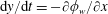 $\text{d}y/\text{d}t=-\unicode[STIX]{x2202}\unicode[STIX]{x1D719}_{w}/\unicode[STIX]{x2202}x$
with the initial condition
$\text{d}y/\text{d}t=-\unicode[STIX]{x2202}\unicode[STIX]{x1D719}_{w}/\unicode[STIX]{x2202}x$
with the initial condition
 $x(x_{s},y_{s},t=0)=x_{s}$
and
$x(x_{s},y_{s},t=0)=x_{s}$
and
 $y(x_{s},y_{s},t=0)=y_{s}$
. Conventionally, a wave equation is written using partial rather than total derivatives. This can be done by noting
$y(x_{s},y_{s},t=0)=y_{s}$
. Conventionally, a wave equation is written using partial rather than total derivatives. This can be done by noting
 $\text{d}/\text{d}t=(\unicode[STIX]{x2202}/\unicode[STIX]{x2202}t)_{x_{s},y_{s}}$
and
$\text{d}/\text{d}t=(\unicode[STIX]{x2202}/\unicode[STIX]{x2202}t)_{x_{s},y_{s}}$
and
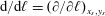 $\text{d}/\text{d}\ell =(\unicode[STIX]{x2202}/\unicode[STIX]{x2202}\ell )_{x_{s},y_{s}}$
.
$\text{d}/\text{d}\ell =(\unicode[STIX]{x2202}/\unicode[STIX]{x2202}\ell )_{x_{s},y_{s}}$
.
3.5.1 General Alfvén wave solution
Along each magnetic field line, which means for each
 $(x_{s},y_{s})$
, the general solution to equation (3.45) is a sum of two functions of one variable
$(x_{s},y_{s})$
, the general solution to equation (3.45) is a sum of two functions of one variable
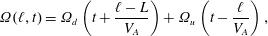 $$\begin{eqnarray}\unicode[STIX]{x1D6FA}(\ell ,t)=\unicode[STIX]{x1D6FA}_{d}\left(t+\frac{\ell -L}{V_{A}}\right)+\unicode[STIX]{x1D6FA}_{u}\left(t-\frac{\ell }{V_{A}}\right),\end{eqnarray}$$
where
 $\unicode[STIX]{x1D6FA}_{d}$
represents a downward going and
$\unicode[STIX]{x1D6FA}_{d}$
represents a downward going and
 $\unicode[STIX]{x1D6FA}_{u}$
an upward going Alfvén wave. The two boundary conditions that determine
$\unicode[STIX]{x1D6FA}_{u}$
an upward going Alfvén wave. The two boundary conditions that determine
 $\unicode[STIX]{x1D6FA}_{d}$
and
$\unicode[STIX]{x1D6FA}_{d}$
and
 $\unicode[STIX]{x1D6FA}_{u}$
are
$\unicode[STIX]{x1D6FA}_{u}$
are
 $\unicode[STIX]{x1D6FA}(z=0,t)=0$
and
$\unicode[STIX]{x1D6FA}(z=0,t)=0$
and
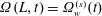 $\unicode[STIX]{x1D6FA}(L,t)=\unicode[STIX]{x1D6FA}_{w}^{(s)}(t)$
, where
$\unicode[STIX]{x1D6FA}(L,t)=\unicode[STIX]{x1D6FA}_{w}^{(s)}(t)$
, where
 $\unicode[STIX]{x1D6FA}_{w}^{(s)}(t)$
is the vorticity of the flow in the wall at the location given by
$\unicode[STIX]{x1D6FA}_{w}^{(s)}(t)$
is the vorticity of the flow in the wall at the location given by
 $(x_{s},y_{s})$
at
$(x_{s},y_{s})$
at
 $\ell =0$
. The vorticity of the flow in the wall is
$\ell =0$
. The vorticity of the flow in the wall is
 $\unicode[STIX]{x1D6FA}_{w}(x,y,t)=-\unicode[STIX]{x1D6FB}^{2}\unicode[STIX]{x1D719}_{w}(x,y,t)$
, and
$\unicode[STIX]{x1D6FA}_{w}(x,y,t)=-\unicode[STIX]{x1D6FB}^{2}\unicode[STIX]{x1D719}_{w}(x,y,t)$
, and
 $\unicode[STIX]{x1D6FA}_{w}^{(s)}(t)=\unicode[STIX]{x1D6FA}_{w}\left(x(x_{s},y_{s},t),y(x_{s},y_{s},t),t\right)$
.
$\unicode[STIX]{x1D6FA}_{w}^{(s)}(t)=\unicode[STIX]{x1D6FA}_{w}\left(x(x_{s},y_{s},t),y(x_{s},y_{s},t),t\right)$
.
The solution assuming the flow in the wall is zero for
 $t<0$
is
$t<0$
is
 $$\begin{eqnarray}\displaystyle \unicode[STIX]{x1D6FA}_{d}(t) & = & \displaystyle \unicode[STIX]{x1D6FA}_{w}^{(s)}(t)\quad \text{for }t<\frac{2L}{V_{A}}\end{eqnarray}$$
 $$\begin{eqnarray}\displaystyle \unicode[STIX]{x1D6FA}_{d}(t) & = & \displaystyle \unicode[STIX]{x1D6FA}_{w}^{(s)}(t)+\unicode[STIX]{x1D6FA}_{d}\left(t-\frac{2L}{V_{A}}\right)\quad \text{for }t>\frac{2L}{V_{A}}\end{eqnarray}$$
 $$\begin{eqnarray}\displaystyle \unicode[STIX]{x1D6FA}_{u}(t) & = & \displaystyle -\unicode[STIX]{x1D6FA}_{d}\left(t-\frac{L}{V_{A}}\right)\quad \text{for }t>\frac{L}{V_{A}}.\end{eqnarray}$$
When the vorticity of the wall flow evolves slowly compared to the Alfvén transit time,
 $\unicode[STIX]{x1D70F}_{A}\equiv L/V_{A}$
:
$\unicode[STIX]{x1D70F}_{A}\equiv L/V_{A}$
:
 $$\begin{eqnarray}\displaystyle \frac{\text{d}\unicode[STIX]{x1D6FA}_{d}(t)}{\text{d}t} & = & \displaystyle \frac{\unicode[STIX]{x1D6FA}_{w}^{(s)}(t)}{2\unicode[STIX]{x1D70F}_{A}}\end{eqnarray}$$
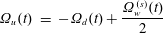 $$\begin{eqnarray}\displaystyle \unicode[STIX]{x1D6FA}_{u}(t) & = & \displaystyle -\unicode[STIX]{x1D6FA}_{d}(t)+\frac{\unicode[STIX]{x1D6FA}_{w}^{(s)}(t)}{2}\end{eqnarray}$$
 $$\begin{eqnarray}\displaystyle \unicode[STIX]{x1D6FA}(\ell ,t) & = & \displaystyle \unicode[STIX]{x1D6FA}_{w}^{(s)}(t)\frac{\ell }{L}\end{eqnarray}$$
 $$\begin{eqnarray}\displaystyle \frac{\text{d}K}{\text{d}t} & = & \displaystyle \frac{\unicode[STIX]{x1D6FA}_{w}^{(s)}(t)}{L}.\end{eqnarray}$$
3.5.2 Discussion of ideal solution and its breaking
The function
 $\unicode[STIX]{x1D6FA}_{w}^{(s)}(t)$
is purely determined by the properties of the flow in the perfectly conducting wall at
$\unicode[STIX]{x1D6FA}_{w}^{(s)}(t)$
is purely determined by the properties of the flow in the perfectly conducting wall at
 $z=L$
. Once
$z=L$
. Once
 $\unicode[STIX]{x1D6FA}_{w}^{(s)}(t)$
is known, a solution for
$\unicode[STIX]{x1D6FA}_{w}^{(s)}(t)$
is known, a solution for
 $K(x_{s},y_{s},\ell ,t)$
is determined, essentially analytically, by (3.46) to (3.49). The solution for the magnetic field lines
$K(x_{s},y_{s},\ell ,t)$
is determined, essentially analytically, by (3.46) to (3.49). The solution for the magnetic field lines
 $\boldsymbol{x}_{\bot }(x_{s},y_{s},z,t)$
in the region
$\boldsymbol{x}_{\bot }(x_{s},y_{s},z,t)$
in the region
 $0<z<L$
requires the Hamiltonian
$0<z<L$
requires the Hamiltonian
 $H(x,y,z,t)$
. The direct solution for Hamiltonian
$H(x,y,z,t)$
. The direct solution for Hamiltonian
 $H_{d}(x,y,z)$
, which can be obtained from
$H_{d}(x,y,z)$
, which can be obtained from
 $K(x_{s},y_{s},\ell )$
using (3.30) to (3.33), will not be exact and small adjustments will generally be required for the field lines started at
$K(x_{s},y_{s},\ell )$
using (3.30) to (3.33), will not be exact and small adjustments will generally be required for the field lines started at
 $(x_{s},y_{s})$
to reach the required positions at
$(x_{s},y_{s})$
to reach the required positions at
 $z=L$
. One way to do this is to let
$z=L$
. One way to do this is to let
 $H(x,y,z)=H_{d}(x,y,z)+\unicode[STIX]{x1D6FF}H(x,y)$
. The function
$H(x,y,z)=H_{d}(x,y,z)+\unicode[STIX]{x1D6FF}H(x,y)$
. The function
 $\unicode[STIX]{x1D6FF}H$
has sufficient freedom to achieve an exact match of the field lines between their starting and ending position.
$\unicode[STIX]{x1D6FF}H$
has sufficient freedom to achieve an exact match of the field lines between their starting and ending position.
 $K$
is modified by
$K$
is modified by
 $\unicode[STIX]{x1D6FF}H$
, but presumably the modification is small when a solution is accurately calculated.
$\unicode[STIX]{x1D6FF}H$
, but presumably the modification is small when a solution is accurately calculated.
This slowly evolving solution need not be the only solution. Indeed it is not unique when the system has an ideal instability (Huang, Bhattacharjee & Boozer Reference Huang, Bhattacharjee and Boozer2014), which allows for a change in the magnetic configuration on a time scale set by the Alfvén transit time
 $L/V_{A}$
. The importance of ideal instabilities in fast magnetic reconnection needs to be better understood.
$L/V_{A}$
. The importance of ideal instabilities in fast magnetic reconnection needs to be better understood.
As discussed in §§ 1 and 2, the properties of the ideal solution determine a large part of the theory of fast magnetic reconnection – even when non-ideal effects become important. The ideality of the magnetic evolution, when expressed by the relation
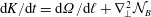 $\text{d}K/\text{d}t=\text{d}\unicode[STIX]{x1D6FA}/\text{d}\ell +\unicode[STIX]{x1D6FB}_{\bot }^{2}{\mathcal{N}}_{B}$
, is broken when the diffusive term
$\text{d}K/\text{d}t=\text{d}\unicode[STIX]{x1D6FA}/\text{d}\ell +\unicode[STIX]{x1D6FB}_{\bot }^{2}{\mathcal{N}}_{B}$
, is broken when the diffusive term
 $\unicode[STIX]{x1D6FB}_{\bot }^{2}{\mathcal{N}}_{B}$
becomes comparable to
$\unicode[STIX]{x1D6FB}_{\bot }^{2}{\mathcal{N}}_{B}$
becomes comparable to
 $\text{d}K/\text{d}t$
for terms in
$\text{d}K/\text{d}t$
for terms in
 $K$
that have a small
$K$
that have a small
 $\boldsymbol{k}_{\bot }$
. Alfvén speed relaxation is modified by viscosity when the diffusive term for the vorticity
$\boldsymbol{k}_{\bot }$
. Alfvén speed relaxation is modified by viscosity when the diffusive term for the vorticity
 $\unicode[STIX]{x1D708}_{v}\unicode[STIX]{x1D6FB}_{\bot }^{2}\unicode[STIX]{x1D6FA}$
has a similar relation to small
$\unicode[STIX]{x1D708}_{v}\unicode[STIX]{x1D6FB}_{\bot }^{2}\unicode[STIX]{x1D6FA}$
has a similar relation to small
 $\boldsymbol{k}_{\bot }$
terms in
$\boldsymbol{k}_{\bot }$
terms in
 $\unicode[STIX]{x1D6FA}$
. The complexity of the geometry when
$\unicode[STIX]{x1D6FA}$
. The complexity of the geometry when
 $\unicode[STIX]{x1D70E}$
is large implies the
$\unicode[STIX]{x1D70E}$
is large implies the
 $\unicode[STIX]{x1D6FB}_{\bot }^{2}$
operator becomes large indeed, equation (3.28), even when the streamlines in the flowing boundary do not themselves exponentiate apart, as when
$\unicode[STIX]{x1D6FB}_{\bot }^{2}$
operator becomes large indeed, equation (3.28), even when the streamlines in the flowing boundary do not themselves exponentiate apart, as when
 $\unicode[STIX]{x1D719}_{w}$
is independent of time. The complexity is even greater when the streamlines do exponentiate apart, and it is important to understand the effect of streamline exponentiation on reconnection.
$\unicode[STIX]{x1D719}_{w}$
is independent of time. The complexity is even greater when the streamlines do exponentiate apart, and it is important to understand the effect of streamline exponentiation on reconnection.
3.6 Dimensionless ratios
The drive for reconnection in the simple model of § 3 is the flow
 $\boldsymbol{v}_{w}=\unicode[STIX]{x1D735}\unicode[STIX]{x1D719}_{w}\times \hat{z}$
in the wall, which is often assumed to be very slow
$\boldsymbol{v}_{w}=\unicode[STIX]{x1D735}\unicode[STIX]{x1D719}_{w}\times \hat{z}$
in the wall, which is often assumed to be very slow
 $$\begin{eqnarray}M_{eff}\equiv \frac{v_{w}L}{V_{A}a_{c}}\ll 1,\end{eqnarray}$$
where
 $a_{c}$
is the characteristic spatial scale for variations in
$a_{c}$
is the characteristic spatial scale for variations in
 $\unicode[STIX]{x1D719}_{w}$
.
$\unicode[STIX]{x1D719}_{w}$
.
By definition, an ideal magnetic evolution can move the magnetic field lines but cannot break them. The expression for the electric field has two terms that break the ideal evolution of the magnetic field. The dimensionless coefficients that give the strength of this breaking are the magnetic Reynolds number,
 $$\begin{eqnarray}\displaystyle & \displaystyle R_{m}\equiv \frac{a_{c}v_{w}}{\unicode[STIX]{x1D702}/\unicode[STIX]{x1D707}_{0}}, & \displaystyle\end{eqnarray}$$
 $$\begin{eqnarray}\displaystyle & \displaystyle \text{and}\quad \frac{a_{c}}{c/\unicode[STIX]{x1D714}_{\text{pe}}}. & \displaystyle\end{eqnarray}$$
Both dimensionless coefficients must be very large compared to unity to have a non-trivial reconnection problem.
The viscosity
 $\unicode[STIX]{x1D708}_{v}$
breaks the ideal equation for the plasma flow and has the Reynolds number as its dimensionless coefficient,
$\unicode[STIX]{x1D708}_{v}$
breaks the ideal equation for the plasma flow and has the Reynolds number as its dimensionless coefficient,
 $$\begin{eqnarray}R_{e}\equiv \frac{a_{c}v_{w}}{\unicode[STIX]{x1D708}_{v}}.\end{eqnarray}$$
A non-trivial problem in magnetic reconnection exists for any value of
 $R_{e}$
. The strength of the viscosity is sometimes given by the magnetic Prandtl number
$R_{e}$
. The strength of the viscosity is sometimes given by the magnetic Prandtl number
 $P_{m}\equiv \unicode[STIX]{x1D707}_{0}\unicode[STIX]{x1D708}_{v}/\unicode[STIX]{x1D702}$
, which can be very large compared to unity in plasmas. A more important parameter in measuring the relative importance of viscous to resistive dissipation will be found to be the Alfvén-weighted Prandtl number,
$P_{m}\equiv \unicode[STIX]{x1D707}_{0}\unicode[STIX]{x1D708}_{v}/\unicode[STIX]{x1D702}$
, which can be very large compared to unity in plasmas. A more important parameter in measuring the relative importance of viscous to resistive dissipation will be found to be the Alfvén-weighted Prandtl number,
 $$\begin{eqnarray}\displaystyle {\mathcal{P}}_{A} & \equiv & \displaystyle M_{eff}^{2}P_{m}\nonumber\\ \displaystyle & = & \displaystyle \left(\frac{v_{w}L}{a_{c}V_{A}}\right)^{2}\frac{\unicode[STIX]{x1D707}_{0}\unicode[STIX]{x1D708}_{v}}{\unicode[STIX]{x1D702}}.\end{eqnarray}$$
3.7 Alfvén waves with dissipation
When the magnetic field evolution is non-ideal, there is a slippage between the magnetic field lines and the plasma, so
 $\text{d}/\text{d}\ell$
and
$\text{d}/\text{d}\ell$
and
 $\text{d}/\text{d}t$
no longer commute. Equation (D 8) implies
$\text{d}/\text{d}t$
no longer commute. Equation (D 8) implies
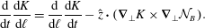 $$\begin{eqnarray}\frac{\text{d}}{\text{d}t}\frac{\text{d}K}{\text{d}\ell }=\frac{\text{d}}{\text{d}\ell }\frac{\text{d}K}{\text{d}t}-\hat{z}\boldsymbol{\cdot }(\unicode[STIX]{x1D735}_{\bot }K\times \unicode[STIX]{x1D735}_{\bot }{\mathcal{N}}_{B}).\end{eqnarray}$$
Equations (3.27) and (3.40) then give the equation for Alfvén waves with dissipation
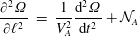 $$\begin{eqnarray}\displaystyle \frac{\unicode[STIX]{x2202}^{2}\unicode[STIX]{x1D6FA}}{\unicode[STIX]{x2202}\ell ^{2}} & = & \displaystyle \frac{1}{V_{A}^{2}}\frac{\text{d}^{2}\unicode[STIX]{x1D6FA}}{\text{d}t^{2}}+{\mathcal{N}}_{A}\end{eqnarray}$$
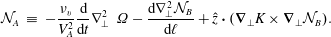 $$\begin{eqnarray}\displaystyle {\mathcal{N}}_{A} & \equiv & \displaystyle -\frac{\unicode[STIX]{x1D708}_{v}}{V_{A}^{2}}\frac{\text{d}}{\text{d}t}\unicode[STIX]{x1D6FB}_{\bot }^{2}~\unicode[STIX]{x1D6FA}-\frac{\text{d}\unicode[STIX]{x1D6FB}_{\bot }^{2}{\mathcal{N}}_{B}}{\text{d}\ell }+\hat{z}\boldsymbol{\cdot }(\unicode[STIX]{x1D735}_{\bot }K\times \unicode[STIX]{x1D735}_{\bot }{\mathcal{N}}_{B}).\end{eqnarray}$$
The two dissipative terms, one proportional to
 $\unicode[STIX]{x1D708}_{v}$
and the other proportional to
$\unicode[STIX]{x1D708}_{v}$
and the other proportional to
 $\unicode[STIX]{x1D702}/\unicode[STIX]{x1D707}_{0}$
, have a ratio of the Alfvén-weighted Prandtl number
$\unicode[STIX]{x1D702}/\unicode[STIX]{x1D707}_{0}$
, have a ratio of the Alfvén-weighted Prandtl number
 ${\mathcal{P}}_{A}$
, equation (3.58), which follows from
${\mathcal{P}}_{A}$
, equation (3.58), which follows from
 $H\sim a_{c}^{2}/L$
and
$H\sim a_{c}^{2}/L$
and
 $\unicode[STIX]{x1D6FA}\sim v_{w}/a_{c}$
. The term
$\unicode[STIX]{x1D6FA}\sim v_{w}/a_{c}$
. The term
 $\text{d}^{2}\unicode[STIX]{x1D6FA}/\text{d}t^{2}$
has a relative size comparable to the viscosity term of the Reynold number
$\text{d}^{2}\unicode[STIX]{x1D6FA}/\text{d}t^{2}$
has a relative size comparable to the viscosity term of the Reynold number
 $R_{e}$
.
$R_{e}$
.
When the viscosity dominates over resistivity in the damping of Alfveń waves, equation (3.60) can be written in a particularly simple form
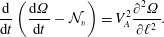 $$\begin{eqnarray}\frac{\text{d}}{\text{d}t}\left(\frac{\text{d}\unicode[STIX]{x1D6FA}}{\text{d}t}-{\mathcal{N}}_{v}\right)=V_{A}^{2}\frac{\unicode[STIX]{x2202}^{2}\unicode[STIX]{x1D6FA}}{\unicode[STIX]{x2202}\ell ^{2}}.\end{eqnarray}$$
3.8 Difficulty of obtaining solutions
The evolution of the model for a driven magnetic field can be obtained by integration until the number of exponentiations
 $\unicode[STIX]{x1D70E}$
in the separation between neighbouring magnetic field lines becomes large. Unfortunately, the difficulty of following the evolution increases as
$\unicode[STIX]{x1D70E}$
in the separation between neighbouring magnetic field lines becomes large. Unfortunately, the difficulty of following the evolution increases as
 $e^{5\unicode[STIX]{x1D70E}}$
, so a hard cutoff exists in the maximum value of
$e^{5\unicode[STIX]{x1D70E}}$
, so a hard cutoff exists in the maximum value of
 $\unicode[STIX]{x1D70E}$
that can be resolved. To follow the evolution, high numerical precision is required; numerical errors blur the evolution of magnetic field lines as does
$\unicode[STIX]{x1D70E}$
that can be resolved. To follow the evolution, high numerical precision is required; numerical errors blur the evolution of magnetic field lines as does
 $c/\unicode[STIX]{x1D714}_{\text{pe}}$
.
$c/\unicode[STIX]{x1D714}_{\text{pe}}$
.
A petascale computer can perform
 $10^{15}$
operations a second or
$10^{15}$
operations a second or
 ${\approx}10^{26}$
per day. When
${\approx}10^{26}$
per day. When
 $\unicode[STIX]{x1D70E}=10$
, the number of operations is increased by approximately
$\unicode[STIX]{x1D70E}=10$
, the number of operations is increased by approximately
 $10^{22}$
times over the case when
$10^{22}$
times over the case when
 $\unicode[STIX]{x1D70E}\lesssim 1$
, so
$\unicode[STIX]{x1D70E}\lesssim 1$
, so
 $\unicode[STIX]{x1D70E}\approx 10$
appears to be an upper limit on what can be computed. Increasing the computer power by a thousand increases the maximum computable
$\unicode[STIX]{x1D70E}\approx 10$
appears to be an upper limit on what can be computed. Increasing the computer power by a thousand increases the maximum computable
 $\unicode[STIX]{x1D70E}$
from
$\unicode[STIX]{x1D70E}$
from
 $\unicode[STIX]{x1D70E}\approx 10$
to
$\unicode[STIX]{x1D70E}\approx 10$
to
 $\unicode[STIX]{x1D70E}\approx 11.4$
.
$\unicode[STIX]{x1D70E}\approx 11.4$
.
Reaching values of
 $\unicode[STIX]{x1D70E}\approx 8$
for studying magnetic reconnection in fusion devices is credible, but
$\unicode[STIX]{x1D70E}\approx 8$
for studying magnetic reconnection in fusion devices is credible, but
 $\unicode[STIX]{x1D70E}\approx 20$
, which is required to understand reconnection in the corona, appears impossible. Simulations using modest values of
$\unicode[STIX]{x1D70E}\approx 20$
, which is required to understand reconnection in the corona, appears impossible. Simulations using modest values of
 $\unicode[STIX]{x1D70E}$
must be sufficiently well understood to devise extrapolations or reliable approximations.
$\unicode[STIX]{x1D70E}$
must be sufficiently well understood to devise extrapolations or reliable approximations.
Once
 $\unicode[STIX]{x1D70E}$
becomes large, distances in the
$\unicode[STIX]{x1D70E}$
becomes large, distances in the
 $(x,y)$
plane of order
$(x,y)$
plane of order
 $a_{c}e^{-\unicode[STIX]{x1D70E}}$
must be resolved as must distances of order
$a_{c}e^{-\unicode[STIX]{x1D70E}}$
must be resolved as must distances of order
 $Le^{-\unicode[STIX]{x1D70E}}$
in the
$Le^{-\unicode[STIX]{x1D70E}}$
in the
 $z$
direction. The speed with which the magnetic field lines move is of order
$z$
direction. The speed with which the magnetic field lines move is of order
 $v_{w}e^{\unicode[STIX]{x1D70E}}$
, so the time required for a field line to move over a spatial scale
$v_{w}e^{\unicode[STIX]{x1D70E}}$
, so the time required for a field line to move over a spatial scale
 $a_{c}e^{-\unicode[STIX]{x1D70E}}$
is
$a_{c}e^{-\unicode[STIX]{x1D70E}}$
is
 $(a_{c}/v_{w})e^{-2\unicode[STIX]{x1D70E}}$
. Assuming the computational difficulty scales as the number of spatial grid cells times the number of time steps, the difficulty scales as
$(a_{c}/v_{w})e^{-2\unicode[STIX]{x1D70E}}$
. Assuming the computational difficulty scales as the number of spatial grid cells times the number of time steps, the difficulty scales as
 $e^{5\unicode[STIX]{x1D70E}}$
.
$e^{5\unicode[STIX]{x1D70E}}$
.
4 Discussion
When dissipation is low, Alfvénic reconnection is so prevalent that it must be a natural consequence of an ideal evolution. The most important result of the paper is the proof that this is indeed the case, § 2.
The sixty-year focus on two-coordinate models to represent magnetic reconnection in three-dimensional space has obscured physics. The generic tendency for evolving magnetic fields to reach states with Alfvén speed reconnection is eliminated by restricting the evolution to a two-coordinate space. Two-coordinate models of magnetic reconnection may be adequate to describe some features of reconnection, but are obviously only an approximation in three-dimensional space. The range of validity of two-dimensional models can only be established by derivations that begin with all three spatial dimensions.
The most important effect eliminated by a two-dimensional approximation is the exponentially large distortion of infinitesimal magnetic flux tubes with distance along the tube. As shown in § 2.1, the exponential enhancement of reconnection in three spatial dimensions is analogous to the increase in mixing of incompressible fluids produced by time depending stirring in two-dimensional models.
The absence of studies of how ideally evolving magnetic fields go from smooth initial to Alfvénic reconnecting states makes simple models of profound importance. Even heuristic arguments, such as those given in the introduction and § C.3, show that any star with evolving magnetic fields in the photosphere on a much longer spatial scale than a gravitational scale height must have a corona. Calculations could clarify whether this explains the height of the transition region and the electron energy in the corona of the Sun.
Many questions on driven reconnection that remain unanswered could be answered in the driven reconnection model derived in § 3. This model is based on a paper by van Ballegooijen (Reference van Ballegooijen1985). The equations have been studied by a number of authors, notably Ng et al. (Reference Ng, Lin and Bhattacharjee2012) and Huang et al. (Reference Huang, Bhattacharjee and Boozer2014). The study by Huang et al is closely related to the model discussed here but was limited to exponentiations
 $\unicode[STIX]{x1D70E}\lesssim 6$
. Daughton et al. (Reference Daughton, Nakamura, Karimabadi, Roytershteyn and Loring2014) have done extensive kinetic calculations of magnetic reconnection in a more complete magnetic field model retaining all three spatial coordinates, but a Harris sheet was used as an initial condition, and the number of exponentiations was
$\unicode[STIX]{x1D70E}\lesssim 6$
. Daughton et al. (Reference Daughton, Nakamura, Karimabadi, Roytershteyn and Loring2014) have done extensive kinetic calculations of magnetic reconnection in a more complete magnetic field model retaining all three spatial coordinates, but a Harris sheet was used as an initial condition, and the number of exponentiations was
 $\unicode[STIX]{x1D70E}\lesssim 8$
. No studies have been done that follow a smooth initial into a rapidly reconnecting state – even the ideal part of that evolution has not been followed, which as shown in § 3.5, can be greatly simplified by analytic methods.
$\unicode[STIX]{x1D70E}\lesssim 8$
. No studies have been done that follow a smooth initial into a rapidly reconnecting state – even the ideal part of that evolution has not been followed, which as shown in § 3.5, can be greatly simplified by analytic methods.
A number of questions need to be addressed and many could be within the model given in § 3.
(i) How does the parallel-current density increase as the system evolves?
The parallel-current density is the part that directly affects reconnection and its increase is determined by (3.27). Although reconnection generally reaches an Alfvénic rate within the reconnection model of this paper, it appears difficult to produce a singular current density.
(ii) How does the reconnection depend on the three dimensionless parameters
 $R_{m}$
,
$R_{m}$
,
 ${\mathcal{P}}_{A}$
and
${\mathcal{P}}_{A}$
and
 $M_{eff}$
?
$M_{eff}$
?
Reconnection is trivial unless the magnetic Reynolds number
 $R_{m}$
is very large compared to unity, but the complexity of the behaviour as
$R_{m}$
is very large compared to unity, but the complexity of the behaviour as
 $R_{m}\rightarrow \infty$
is poorly understood. Unless the plasma has significant dissipation, the energy released by the reconnection will drive strong Alfvén waves. These waves propagate along the magnetic field lines and develop an extremely complicated spatial dependence and enhanced dissipation from exponentially increasing separation of the lines (Similon & Sudan Reference Similon and Sudan1989).
$R_{m}\rightarrow \infty$
is poorly understood. Unless the plasma has significant dissipation, the energy released by the reconnection will drive strong Alfvén waves. These waves propagate along the magnetic field lines and develop an extremely complicated spatial dependence and enhanced dissipation from exponentially increasing separation of the lines (Similon & Sudan Reference Similon and Sudan1989).
Significant dissipation with a very large magnetic Reynolds number requires the Alfvén-weighted Prandtl number
 ${\mathcal{P}}_{A}$
be large. The dependence of reconnection phenomena on
${\mathcal{P}}_{A}$
be large. The dependence of reconnection phenomena on
 ${\mathcal{P}}_{A}$
is not understood. Although the Alfvénic Mach number
${\mathcal{P}}_{A}$
is not understood. Although the Alfvénic Mach number
 $M_{eff}$
is generally assumed to be small compared to unity, the actual plasma flow can become large due to the large spatial excursions made by magnetic field lines. Indeed, the plasma may become unstable (Huang et al.
Reference Huang, Bhattacharjee and Boozer2014) and make a transition to a different state on an Alfvénic time scale.
$M_{eff}$
is generally assumed to be small compared to unity, the actual plasma flow can become large due to the large spatial excursions made by magnetic field lines. Indeed, the plasma may become unstable (Huang et al.
Reference Huang, Bhattacharjee and Boozer2014) and make a transition to a different state on an Alfvénic time scale.
(iii) How does the reconnection depend on the complexity of the drive
 $\unicode[STIX]{x1D719}_{w}(x,y,t)$
?
$\unicode[STIX]{x1D719}_{w}(x,y,t)$
?
An important but poorly understood question is, when the drive
 $\unicode[STIX]{x1D719}_{w}$
continues for a long time, does the reconnection settle into a quasi-steady state or is it episodic? A finite time, the trigger time, is clearly required to obtain the first reconnection event when the initial condition is
$\unicode[STIX]{x1D719}_{w}$
continues for a long time, does the reconnection settle into a quasi-steady state or is it episodic? A finite time, the trigger time, is clearly required to obtain the first reconnection event when the initial condition is
 $H=0$
. The dependence of the trigger time on either the dimensionless parameters or the complexity of
$H=0$
. The dependence of the trigger time on either the dimensionless parameters or the complexity of
 $\unicode[STIX]{x1D719}_{w}$
is essentially unknown.
$\unicode[STIX]{x1D719}_{w}$
is essentially unknown.
Is the reconnection behaviour qualitatively similar for all functions
 $\unicode[STIX]{x1D719}_{w}(x,y,t)$
that have a similar characteristic spatial scale
$\unicode[STIX]{x1D719}_{w}(x,y,t)$
that have a similar characteristic spatial scale
 $a_{c}$
? When
$a_{c}$
? When
 $\unicode[STIX]{x1D719}_{w}(x,y,t)$
depends on time, neighbouring points in the flowing wall generically separate exponentially in time; when
$\unicode[STIX]{x1D719}_{w}(x,y,t)$
depends on time, neighbouring points in the flowing wall generically separate exponentially in time; when
 $\unicode[STIX]{x1D719}_{w}$
has no time dependence neighbouring wall points do not exponentiate apart. Does this produce a qualitative difference in the reconnection?
$\unicode[STIX]{x1D719}_{w}$
has no time dependence neighbouring wall points do not exponentiate apart. Does this produce a qualitative difference in the reconnection?
When the dominant spatial scale
 $a_{c}$
of
$a_{c}$
of
 $\unicode[STIX]{x1D719}_{w}$
is small compared to the size
$\unicode[STIX]{x1D719}_{w}$
is small compared to the size
 $a$
of the reconnecting region, which may be a periodicity length
$a$
of the reconnecting region, which may be a periodicity length
 $2\unicode[STIX]{x03C0}a$
, the reconnection has a relatively slow diffusive nature, but this is not well understood.
$2\unicode[STIX]{x03C0}a$
, the reconnection has a relatively slow diffusive nature, but this is not well understood.
(iv) Do the short wavelength structures that are driven by fast reconnection in three dimensions play an important role by modifying the timing and the nature of the breaking of the ideal constraints?
When neighbouring field lines exponentiate apart by a factor
 $e^{\unicode[STIX]{x1D70E}}$
, structures are strongly driven on the scale
$e^{\unicode[STIX]{x1D70E}}$
, structures are strongly driven on the scale
 $a_{c}e^{-\unicode[STIX]{x1D70E}}$
.
$a_{c}e^{-\unicode[STIX]{x1D70E}}$
.
(v) How quickly do plasma elements that originally lay along one field line spread across the reconnecting volume?
The rapid spreading of impurities across a tokamak plasma during a disruption is poorly understood but may be a by-product of the fast magnetic reconnection that is associated with the current spike (Boozer Reference Boozer2017).
(vi) Under what conditions does
 $c/\unicode[STIX]{x1D714}_{\text{pe}}$
dominate the resistivity
$c/\unicode[STIX]{x1D714}_{\text{pe}}$
dominate the resistivity
 $\unicode[STIX]{x1D702}$
in causing magnetic field line breaking?
$\unicode[STIX]{x1D702}$
in causing magnetic field line breaking?
The large magnetic field line excursions that occur when
 $\unicode[STIX]{x1D70E}$
is large can give large flow velocities and make the time derivative term involving
$\unicode[STIX]{x1D70E}$
is large can give large flow velocities and make the time derivative term involving
 $c/\unicode[STIX]{x1D714}_{\text{pe}}$
far more important than it appears to be.
$c/\unicode[STIX]{x1D714}_{\text{pe}}$
far more important than it appears to be.
(vii) When
 $\unicode[STIX]{x1D719}_{w}$
has a form that gives episodic rather than quasi-steady-state reconnection, how quickly is equilibrium,
$\unicode[STIX]{x1D719}_{w}$
has a form that gives episodic rather than quasi-steady-state reconnection, how quickly is equilibrium,
 $\text{d}K/\text{d}\ell =0$
, re-established?
$\text{d}K/\text{d}\ell =0$
, re-established?
This question is of particular interest in tokamak disruptions because it presumably determines the duration of the current spike (Boozer Reference Boozer2017).
(viii) How is the plasma heating spread over the plasma?
When the magnetic Reynolds number
 $R_{m}$
is very large, reconnection can occur with little dissipation of energy; most of the energy goes first into Alfvén waves. The rapidity with which the Alfvén waves are damped is a complicated issue (Similon & Sudan Reference Similon and Sudan1989; Boozer Reference Boozer2014) but determines both the spatial region and the plasma species that is heated. The results of this paper imply the development of current sheets as described in Boozer (Reference Boozer2014) is incorrect, but the damping of Alfvén waves in nonetheless strong because of the large increase in
$R_{m}$
is very large, reconnection can occur with little dissipation of energy; most of the energy goes first into Alfvén waves. The rapidity with which the Alfvén waves are damped is a complicated issue (Similon & Sudan Reference Similon and Sudan1989; Boozer Reference Boozer2014) but determines both the spatial region and the plasma species that is heated. The results of this paper imply the development of current sheets as described in Boozer (Reference Boozer2014) is incorrect, but the damping of Alfvén waves in nonetheless strong because of the large increase in
 $\unicode[STIX]{x1D6FB}_{\bot }^{2}\unicode[STIX]{x1D6FA}$
due to magnetic field line exponentiation.
$\unicode[STIX]{x1D6FB}_{\bot }^{2}\unicode[STIX]{x1D6FA}$
due to magnetic field line exponentiation.
Acknowledgements
This material is based upon work supported by the U.S. Department of Energy, Office of Science, Office of Fusion Energy Sciences under award nos DE-FG02-95ER54333 and DE-FG02-03ER54696.
Appendix A. Plasma versus magnetic field line velocity
The small gyroradius Ohm’s law,
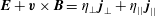 $\boldsymbol{E}+\boldsymbol{v}\times \boldsymbol{B}=\unicode[STIX]{x1D702}_{\bot }\,\boldsymbol{j}_{\bot }+\unicode[STIX]{x1D702}_{||}\,\boldsymbol{j}_{||}$
, illustrates the importance of distinguishing between the plasma velocity
$\boldsymbol{E}+\boldsymbol{v}\times \boldsymbol{B}=\unicode[STIX]{x1D702}_{\bot }\,\boldsymbol{j}_{\bot }+\unicode[STIX]{x1D702}_{||}\,\boldsymbol{j}_{||}$
, illustrates the importance of distinguishing between the plasma velocity
 $\boldsymbol{v}$
and the magnetic field line velocity
$\boldsymbol{v}$
and the magnetic field line velocity
 $\boldsymbol{u}$
. This Ohm’s law can be written as
$\boldsymbol{u}$
. This Ohm’s law can be written as
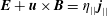 $\boldsymbol{E}+\boldsymbol{u}\times \boldsymbol{B}=\unicode[STIX]{x1D702}_{||}\,\boldsymbol{j}_{||}$
with
$\boldsymbol{E}+\boldsymbol{u}\times \boldsymbol{B}=\unicode[STIX]{x1D702}_{||}\,\boldsymbol{j}_{||}$
with
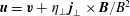 $\boldsymbol{u}=\boldsymbol{v}+\unicode[STIX]{x1D702}_{\bot }\,\boldsymbol{j}_{\bot }\times \boldsymbol{B}/B^{2}$
. The velocity of the plasma
$\boldsymbol{u}=\boldsymbol{v}+\unicode[STIX]{x1D702}_{\bot }\,\boldsymbol{j}_{\bot }\times \boldsymbol{B}/B^{2}$
. The velocity of the plasma
 $\boldsymbol{v}$
is the sum of the velocity of the magnetic field lines and the velocity of the plasma across the lines
$\boldsymbol{v}$
is the sum of the velocity of the magnetic field lines and the velocity of the plasma across the lines
 $-\unicode[STIX]{x1D702}_{\bot }\,\boldsymbol{j}_{\bot }\times \boldsymbol{B}/B^{2}$
. Letting
$-\unicode[STIX]{x1D702}_{\bot }\,\boldsymbol{j}_{\bot }\times \boldsymbol{B}/B^{2}$
. Letting
 $\boldsymbol{j}\times \boldsymbol{B}=\unicode[STIX]{x1D735}p$
and ignoring the temperature gradient, the plasma velocity across the magnetic field lines is
$\boldsymbol{j}\times \boldsymbol{B}=\unicode[STIX]{x1D735}p$
and ignoring the temperature gradient, the plasma velocity across the magnetic field lines is
 $\boldsymbol{v}-\boldsymbol{u}=-D_{cl}\unicode[STIX]{x1D735}n$
. The classical diffusion coefficient
$\boldsymbol{v}-\boldsymbol{u}=-D_{cl}\unicode[STIX]{x1D735}n$
. The classical diffusion coefficient
 $D_{cl}\equiv \unicode[STIX]{x1D702}_{\bot }nT/B^{2}$
can be written as
$D_{cl}\equiv \unicode[STIX]{x1D702}_{\bot }nT/B^{2}$
can be written as
 $D_{cl}=(m_{e}/m_{i})\unicode[STIX]{x1D70C}_{i}^{2}\unicode[STIX]{x1D708}_{c}$
, where
$D_{cl}=(m_{e}/m_{i})\unicode[STIX]{x1D70C}_{i}^{2}\unicode[STIX]{x1D708}_{c}$
, where
 $\unicode[STIX]{x1D70C}_{i}$
is the ion gyroradius and
$\unicode[STIX]{x1D70C}_{i}$
is the ion gyroradius and
 $\unicode[STIX]{x1D708}_{c}$
is the electron collision frequency in
$\unicode[STIX]{x1D708}_{c}$
is the electron collision frequency in
 $\unicode[STIX]{x1D702}_{\bot }$
. In large tokamaks, microturbulence causes particle transport that is of order gyro-Bohm diffusion
$\unicode[STIX]{x1D702}_{\bot }$
. In large tokamaks, microturbulence causes particle transport that is of order gyro-Bohm diffusion
 $D_{gB}=(\unicode[STIX]{x1D70C}_{i}/R_{0})(T/eB)$
, where
$D_{gB}=(\unicode[STIX]{x1D70C}_{i}/R_{0})(T/eB)$
, where
 $R_{0}$
is the major radius. The ratio of the observed to the classical particle transport,
$R_{0}$
is the major radius. The ratio of the observed to the classical particle transport,
 $D_{gB}/D_{cl}=(v_{i}/R_{0})/(m_{e}\unicode[STIX]{x1D70F}_{e}/m_{i})\approx 10^{5}$
, where
$D_{gB}/D_{cl}=(v_{i}/R_{0})/(m_{e}\unicode[STIX]{x1D70F}_{e}/m_{i})\approx 10^{5}$
, where
 $v_{i}$
is the ion thermal speed, so the effective
$v_{i}$
is the ion thermal speed, so the effective
 $\unicode[STIX]{x1D702}_{\bot }$
is enhanced by a factor
$\unicode[STIX]{x1D702}_{\bot }$
is enhanced by a factor
 ${\approx}10^{5}$
over its classical value. Boozer (Reference Boozer2004) has shown slippage of the poloidal compared to the toroidal magnetic flux in tokamaks, which is given by the magnetic field line velocity
${\approx}10^{5}$
over its classical value. Boozer (Reference Boozer2004) has shown slippage of the poloidal compared to the toroidal magnetic flux in tokamaks, which is given by the magnetic field line velocity
 $\boldsymbol{u}$
or equivalently the loop voltage, is determined by
$\boldsymbol{u}$
or equivalently the loop voltage, is determined by
 $\unicode[STIX]{x1D702}_{||}j_{||}$
. The observed parallel resistivity, when corrected by approximately a factor of two for trapped particle effects, is consistent with the classical value of
$\unicode[STIX]{x1D702}_{||}j_{||}$
. The observed parallel resistivity, when corrected by approximately a factor of two for trapped particle effects, is consistent with the classical value of
 $\unicode[STIX]{x1D702}_{||}$
. In other words, in large tokamak experiments
$\unicode[STIX]{x1D702}_{||}$
. In other words, in large tokamak experiments
 $\unicode[STIX]{x1D702}_{\bot }/\unicode[STIX]{x1D702}_{||}\approx 10^{5}$
.
$\unicode[STIX]{x1D702}_{\bot }/\unicode[STIX]{x1D702}_{||}\approx 10^{5}$
.
Appendix B. Relativistic extensions
The Lorentz transformation for the electric and magnetic fields demonstrates that both the concept of a magnetic field line velocity
 $\boldsymbol{u}$
and the anti-reconnection theorem remain valid and important in relativistic theory. Jackson (Reference Jackson1998) in his equation (11.149) gave this Lorentz transformation. When the velocity
$\boldsymbol{u}$
and the anti-reconnection theorem remain valid and important in relativistic theory. Jackson (Reference Jackson1998) in his equation (11.149) gave this Lorentz transformation. When the velocity
 $\boldsymbol{u}$
is perpendicular to both
$\boldsymbol{u}$
is perpendicular to both
 $\boldsymbol{E}$
and
$\boldsymbol{E}$
and
 $\boldsymbol{B}$
, Jackson’s equation implies
$\boldsymbol{B}$
, Jackson’s equation implies
 $$\begin{eqnarray}\displaystyle \boldsymbol{E}_{u} & = & \displaystyle \unicode[STIX]{x1D6FE}(\boldsymbol{E}+\boldsymbol{u}\times \boldsymbol{B});\end{eqnarray}$$
 $$\begin{eqnarray}\displaystyle \boldsymbol{B}_{u} & = & \displaystyle \unicode[STIX]{x1D6FE}\left(\boldsymbol{B}-\frac{1}{c^{2}}\boldsymbol{u}\times \boldsymbol{E}\right).\end{eqnarray}$$
Let
 $\boldsymbol{E}(\boldsymbol{x},t)$
and
$\boldsymbol{E}(\boldsymbol{x},t)$
and
 $\boldsymbol{B}(\boldsymbol{x},t)$
be the electric and magnetic fields in the frame of reference that is the basis of the analysis. The evolution of the magnetic field in that frame,
$\boldsymbol{B}(\boldsymbol{x},t)$
be the electric and magnetic fields in the frame of reference that is the basis of the analysis. The evolution of the magnetic field in that frame,
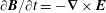 $\unicode[STIX]{x2202}\boldsymbol{B}/\unicode[STIX]{x2202}t=-\unicode[STIX]{x1D735}\times \boldsymbol{E}$
, is identical to that in a plasma in which the electric field is
$\unicode[STIX]{x2202}\boldsymbol{B}/\unicode[STIX]{x2202}t=-\unicode[STIX]{x1D735}\times \boldsymbol{E}$
, is identical to that in a plasma in which the electric field is
 $\boldsymbol{{\mathcal{E}}}=\boldsymbol{E}+\unicode[STIX]{x1D735}\unicode[STIX]{x1D6F7}$
. The electric field
$\boldsymbol{{\mathcal{E}}}=\boldsymbol{E}+\unicode[STIX]{x1D735}\unicode[STIX]{x1D6F7}$
. The electric field
 $\boldsymbol{{\mathcal{E}}}$
will be the basis of the analysis, and the freedom of
$\boldsymbol{{\mathcal{E}}}$
will be the basis of the analysis, and the freedom of
 $\unicode[STIX]{x1D6F7}$
will be used to make
$\unicode[STIX]{x1D6F7}$
will be used to make
 $\boldsymbol{{\mathcal{E}}}\boldsymbol{\cdot }\boldsymbol{B}=0$
, at least locally. Since
$\boldsymbol{{\mathcal{E}}}\boldsymbol{\cdot }\boldsymbol{B}=0$
, at least locally. Since
 $\boldsymbol{{\mathcal{E}}}\boldsymbol{\cdot }\boldsymbol{B}$
is a Lorentz invariant, the transformed quantity
$\boldsymbol{{\mathcal{E}}}\boldsymbol{\cdot }\boldsymbol{B}$
is a Lorentz invariant, the transformed quantity
 $\boldsymbol{{\mathcal{E}}}_{u}\boldsymbol{\cdot }\boldsymbol{B}_{u}=0$
. In the frame moving with a velocity
$\boldsymbol{{\mathcal{E}}}_{u}\boldsymbol{\cdot }\boldsymbol{B}_{u}=0$
. In the frame moving with a velocity
 $\boldsymbol{u}=\boldsymbol{{\mathcal{E}}}\times \boldsymbol{B}/B^{2}$
relative to the first, the perpendicular electric field is zero,
$\boldsymbol{u}=\boldsymbol{{\mathcal{E}}}\times \boldsymbol{B}/B^{2}$
relative to the first, the perpendicular electric field is zero,
 $\boldsymbol{{\mathcal{E}}}_{u}\times \boldsymbol{B}_{u}=0$
, so in that frame
$\boldsymbol{{\mathcal{E}}}_{u}\times \boldsymbol{B}_{u}=0$
, so in that frame
 $\boldsymbol{{\mathcal{E}}}_{u}=0$
, and the magnetic field
$\boldsymbol{{\mathcal{E}}}_{u}=0$
, and the magnetic field
 $\boldsymbol{B}_{u}$
does not evolve. Letting
$\boldsymbol{B}_{u}$
does not evolve. Letting
 $\unicode[STIX]{x1D6FD}\equiv |\boldsymbol{u}|/c$
, one finds that the requirement to make
$\unicode[STIX]{x1D6FD}\equiv |\boldsymbol{u}|/c$
, one finds that the requirement to make
 $\boldsymbol{{\mathcal{E}}}_{u}\times \boldsymbol{B}_{u}=0$
is
$\boldsymbol{{\mathcal{E}}}_{u}\times \boldsymbol{B}_{u}=0$
is
 $\unicode[STIX]{x1D6FD}/(1+\unicode[STIX]{x1D6FD}^{2})=c{\mathcal{E}}B/({\mathcal{E}}^{2}+c^{2}B^{2})$
. A frame in which there is no electric field is only possible when
$\unicode[STIX]{x1D6FD}/(1+\unicode[STIX]{x1D6FD}^{2})=c{\mathcal{E}}B/({\mathcal{E}}^{2}+c^{2}B^{2})$
. A frame in which there is no electric field is only possible when
 $\unicode[STIX]{x1D6FD}={\mathcal{E}}/cB<1.$
When
$\unicode[STIX]{x1D6FD}={\mathcal{E}}/cB<1.$
When
 ${\mathcal{E}}/cB>1$
with
${\mathcal{E}}/cB>1$
with
 $\boldsymbol{{\mathcal{E}}}\boldsymbol{\cdot }\boldsymbol{B}=0$
, there is no magnetic field in a frame moving with velocity
$\boldsymbol{{\mathcal{E}}}\boldsymbol{\cdot }\boldsymbol{B}=0$
, there is no magnetic field in a frame moving with velocity
 $\boldsymbol{u}=c^{2}\boldsymbol{{\mathcal{E}}}\times \boldsymbol{B}/{\mathcal{E}}^{2}$
. The Lorentz invariant
$\boldsymbol{u}=c^{2}\boldsymbol{{\mathcal{E}}}\times \boldsymbol{B}/{\mathcal{E}}^{2}$
. The Lorentz invariant
 $B^{2}-{\mathcal{E}}^{2}/c^{2}$
ensures distinct behaviour depending on whether
$B^{2}-{\mathcal{E}}^{2}/c^{2}$
ensures distinct behaviour depending on whether
 ${\mathcal{E}}/cB$
is greater or less than unity.
${\mathcal{E}}/cB$
is greater or less than unity.
Appendix C. Spherical geometry
C.1 Curl-free magnetic fields
The sphere is the only smooth and bounded shape that has simple solutions to Laplace’s equation,
 $\unicode[STIX]{x1D6FB}^{2}\unicode[STIX]{x1D719}=0$
. In spherical geometry a curl-free magnetic field has the form
$\unicode[STIX]{x1D6FB}^{2}\unicode[STIX]{x1D719}=0$
. In spherical geometry a curl-free magnetic field has the form
 $$\begin{eqnarray}\displaystyle \boldsymbol{B} & = & \displaystyle \unicode[STIX]{x1D735}g;\end{eqnarray}$$
 $$\begin{eqnarray}\displaystyle g & = & \displaystyle \mathop{\sum }_{\ell n}\frac{aB_{\ell }^{n}}{\ell }\left(\frac{r}{a}\right)^{\ell }Y_{\ell }^{n}(\unicode[STIX]{x1D703},\unicode[STIX]{x1D711}),\quad r<a\end{eqnarray}$$
 $$\begin{eqnarray}\displaystyle & = & \displaystyle -\,\mathop{\sum }_{\ell n}\frac{aB_{\ell }^{n}}{\ell +1}\left(\frac{a}{r}\right)^{\ell +1}Y_{\ell }^{n}(\unicode[STIX]{x1D703},\unicode[STIX]{x1D711}),\quad r>a,\end{eqnarray}$$
where the
 $Y_{\ell }^{n}$
are the spherical harmonics. The coefficient
$Y_{\ell }^{n}$
are the spherical harmonics. The coefficient
 $B_{\ell }^{n}$
is uniquely determined by the
$B_{\ell }^{n}$
is uniquely determined by the
 $n\ell$
normal component
$n\ell$
normal component
 $B_{n}(\unicode[STIX]{x1D703},\unicode[STIX]{x1D711})$
of the magnetic field on the
$B_{n}(\unicode[STIX]{x1D703},\unicode[STIX]{x1D711})$
of the magnetic field on the
 $r=a$
surface of the sphere,
$r=a$
surface of the sphere,
 $$\begin{eqnarray}B_{n}(\unicode[STIX]{x1D703},\unicode[STIX]{x1D711})=\mathop{\sum }_{\ell n}B_{\ell }^{n}Y_{\ell }^{n}(\unicode[STIX]{x1D703},\unicode[STIX]{x1D711}).\end{eqnarray}$$
When the magnetic field is symmetric about the axis of the sphere,
 $\unicode[STIX]{x1D711}$
symmetry, only
$\unicode[STIX]{x1D711}$
symmetry, only
 $n=0$
spherical harmonics appear and the vector potential for the magnetic field is
$n=0$
spherical harmonics appear and the vector potential for the magnetic field is
 $$\begin{eqnarray}\displaystyle \boldsymbol{A} & = & \displaystyle \unicode[STIX]{x1D713}\unicode[STIX]{x1D735}\frac{\unicode[STIX]{x1D711}}{2\unicode[STIX]{x03C0}};\end{eqnarray}$$
 $$\begin{eqnarray}\displaystyle \unicode[STIX]{x1D735}\frac{\unicode[STIX]{x1D711}}{2\unicode[STIX]{x03C0}} & = & \displaystyle \frac{\hat{\unicode[STIX]{x1D711}}}{2\unicode[STIX]{x03C0}r\sin \unicode[STIX]{x1D703}};\end{eqnarray}$$
 $$\begin{eqnarray}\displaystyle \boldsymbol{B} & = & \displaystyle \unicode[STIX]{x1D735}\unicode[STIX]{x1D713}\times \unicode[STIX]{x1D735}\frac{\unicode[STIX]{x1D711}}{2\unicode[STIX]{x03C0}}.\end{eqnarray}$$
The magnetic field lines lie in a constant
 $\unicode[STIX]{x1D713}$
and constant
$\unicode[STIX]{x1D713}$
and constant
 $\unicode[STIX]{x1D711}$
plane. The magnetic flux is
$\unicode[STIX]{x1D711}$
plane. The magnetic flux is
 $\unicode[STIX]{x1D713}=\oint \boldsymbol{A}\boldsymbol{\cdot }(\unicode[STIX]{x2202}\boldsymbol{x}/\unicode[STIX]{x2202}\unicode[STIX]{x1D711})\,\text{d}\unicode[STIX]{x1D711}$
. Letting
$\unicode[STIX]{x1D713}=\oint \boldsymbol{A}\boldsymbol{\cdot }(\unicode[STIX]{x2202}\boldsymbol{x}/\unicode[STIX]{x2202}\unicode[STIX]{x1D711})\,\text{d}\unicode[STIX]{x1D711}$
. Letting
 $Y_{\ell }(\unicode[STIX]{x1D703})\equiv Y_{\ell }^{n=0}$
and
$Y_{\ell }(\unicode[STIX]{x1D703})\equiv Y_{\ell }^{n=0}$
and
 $B_{\ell }\equiv B_{\ell }^{0}$
, then one finds by equating the magnetic field derived from
$B_{\ell }\equiv B_{\ell }^{0}$
, then one finds by equating the magnetic field derived from
 $g$
and from
$g$
and from
 $\unicode[STIX]{x1D713}$
,
$\unicode[STIX]{x1D713}$
,
 $$\begin{eqnarray}\displaystyle \unicode[STIX]{x1D713} & = & \displaystyle \mathop{\sum }_{\ell }\unicode[STIX]{x1D713}_{\ell }\left(\frac{r}{a}\right)^{\ell +1}G_{\ell }(\unicode[STIX]{x1D703});\end{eqnarray}$$
 $$\begin{eqnarray}\displaystyle \unicode[STIX]{x1D713}_{\ell } & = & \displaystyle 2\unicode[STIX]{x03C0}a^{2}B_{\ell };\end{eqnarray}$$
 $$\begin{eqnarray}\displaystyle G_{\ell }(\unicode[STIX]{x1D703}) & = & \displaystyle -\frac{\sin \unicode[STIX]{x1D703}}{\ell (\ell +1)}\frac{\text{d}Y_{\ell }}{\text{d}\unicode[STIX]{x1D703}};\end{eqnarray}$$
 $$\begin{eqnarray}\displaystyle \frac{\text{d}G_{\ell }}{\text{d}\unicode[STIX]{x1D703}} & = & \displaystyle \sin \unicode[STIX]{x1D703}Y_{\ell }.\end{eqnarray}$$
C.2 Magnetic nulls
This section will show that magnetic field lines from one magnetic field null,
 $B^{2}=0$
need not strike another null in a short distance even when a second null lies nearby and that magnetic nulls are generically rare in space.
$B^{2}=0$
need not strike another null in a short distance even when a second null lies nearby and that magnetic nulls are generically rare in space.
First, consider the rarity of nulls in space. Using Cartesian coordinates, a magnetic null implies the solution of three equations with three unknowns:
 $B_{x}(x,y,z)=0$
,
$B_{x}(x,y,z)=0$
,
 $B_{y}(x,y,z)=0$
and
$B_{y}(x,y,z)=0$
and
 $B_{z}(x,y,z)=0$
. Three equations with three unknowns are well known to generically have solutions that are discrete if any solutions exist at all. The standard counterexample is a field with perfect symmetry, such a
$B_{z}(x,y,z)=0$
. Three equations with three unknowns are well known to generically have solutions that are discrete if any solutions exist at all. The standard counterexample is a field with perfect symmetry, such a
 $z$
-symmetry, which means
$z$
-symmetry, which means
 $B_{x}$
,
$B_{x}$
,
 $B_{y}$
and
$B_{y}$
and
 $B_{z}$
are independent of
$B_{z}$
are independent of
 $z$
. When all three components vanish at
$z$
. When all three components vanish at
 $x_{0},y_{0}$
, then there is a line null at
$x_{0},y_{0}$
, then there is a line null at
 $(x_{0},y_{0})$
for all
$(x_{0},y_{0})$
for all
 $z$
. The addition of an arbitrarily small
$z$
. The addition of an arbitrarily small
 $z$
-dependent field will break the line null into discrete point nulls. For example,
$z$
-dependent field will break the line null into discrete point nulls. For example,
 $\unicode[STIX]{x1D6FF}B_{x}\propto \sin z$
will break the line null into point nulls, one at
$\unicode[STIX]{x1D6FF}B_{x}\propto \sin z$
will break the line null into point nulls, one at
 $(x_{0},y_{0},z=0)$
and another at
$(x_{0},y_{0},z=0)$
and another at
 $(x_{0},y_{0},z=\unicode[STIX]{x03C0})$
, no matter how small the amplitude of
$(x_{0},y_{0},z=\unicode[STIX]{x03C0})$
, no matter how small the amplitude of
 $\unicode[STIX]{x1D6FF}B_{x}$
.
$\unicode[STIX]{x1D6FF}B_{x}$
.
Second, consider the existence of field lines that connect nulls. When a null exists in a locally curl-free magnetic field, then one can locate a sphere about the null and obtain an isolated null by the magnetic potential
 $g=(aB_{2})/2\left(r/a\right)^{2}Y_{2}(\unicode[STIX]{x1D703})$
, where
$g=(aB_{2})/2\left(r/a\right)^{2}Y_{2}(\unicode[STIX]{x1D703})$
, where
 $Y_{2}\propto \cos ^{2}\unicode[STIX]{x1D703}-1/3$
, the magnetic field has a single null at
$Y_{2}\propto \cos ^{2}\unicode[STIX]{x1D703}-1/3$
, the magnetic field has a single null at
 $r=0$
and the flux
$r=0$
and the flux
 $\unicode[STIX]{x1D713}=0$
. Note
$\unicode[STIX]{x1D713}=0$
. Note
 $B_{r}\propto r(\cos ^{2}\unicode[STIX]{x1D703}-1/3)$
and
$B_{r}\propto r(\cos ^{2}\unicode[STIX]{x1D703}-1/3)$
and
 $B_{\unicode[STIX]{x1D703}}\propto r\sin 2\unicode[STIX]{x1D703}$
. One could include
$B_{\unicode[STIX]{x1D703}}\propto r\sin 2\unicode[STIX]{x1D703}$
. One could include
 $Y_{2}^{n}$
harmonic terms as well, for example
$Y_{2}^{n}$
harmonic terms as well, for example
 $Y_{2}^{2}\propto \sin ^{2}\unicode[STIX]{x1D703}\sin (2\unicode[STIX]{x1D711})$
, but when they are small they introduce no new nulls in the region
$Y_{2}^{2}\propto \sin ^{2}\unicode[STIX]{x1D703}\sin (2\unicode[STIX]{x1D711})$
, but when they are small they introduce no new nulls in the region
 $r<a$
in which the magnetic field is curl free and would make
$r<a$
in which the magnetic field is curl free and would make
 $\unicode[STIX]{x1D713}$
conservation not rigorously valid.
$\unicode[STIX]{x1D713}$
conservation not rigorously valid.
A field with one additional null can be produced, preserving symmetry in
 $\unicode[STIX]{x1D711}$
, by adding a term to the magnetic potential
$\unicode[STIX]{x1D711}$
, by adding a term to the magnetic potential
 $\propto r^{3}Y_{3}(\unicode[STIX]{x1D703})$
, where
$\propto r^{3}Y_{3}(\unicode[STIX]{x1D703})$
, where
 $Y_{3}\propto \cos ^{3}\unicode[STIX]{x1D703}-(3/5)\cos \unicode[STIX]{x1D703}$
. That is,
$Y_{3}\propto \cos ^{3}\unicode[STIX]{x1D703}-(3/5)\cos \unicode[STIX]{x1D703}$
. That is,
 $$\begin{eqnarray}\displaystyle g & = & \displaystyle \frac{aB_{2}}{2}\left(\frac{r}{a}\right)^{2}\left(\cos ^{2}\unicode[STIX]{x1D703}-\frac{1}{3}\right)+\frac{aB_{3}}{3}\left(\frac{r}{a}\right)^{3}\left(\cos ^{3}\unicode[STIX]{x1D703}-\frac{3}{5}\cos \unicode[STIX]{x1D703}\right);\end{eqnarray}$$
 $$\begin{eqnarray}\displaystyle \unicode[STIX]{x1D713} & = & \displaystyle 2\unicode[STIX]{x03C0}a^{2}B_{2}\left(\frac{r}{a}\right)^{3}\frac{\cos ^{3}\unicode[STIX]{x1D703}-\cos \unicode[STIX]{x1D703}}{3}+2\unicode[STIX]{x03C0}a^{2}B_{3}\left(\frac{r}{a}\right)^{4}\frac{\cos ^{4}\unicode[STIX]{x1D703}-\frac{3}{5}\cos ^{2}\unicode[STIX]{x1D703}+\frac{1}{5}}{4}.\end{eqnarray}$$
The first null is at
 $r=0$
and a second null is at
$r=0$
and a second null is at
 $r/a=c_{0}B_{2}/B_{3}$
, where
$r/a=c_{0}B_{2}/B_{3}$
, where
 $c_{0}=2.357\cdots \,$
, and
$c_{0}=2.357\cdots \,$
, and
 $\unicode[STIX]{x1D703}=\unicode[STIX]{x03C0}/4$
. The flux at the first null is
$\unicode[STIX]{x1D703}=\unicode[STIX]{x03C0}/4$
. The flux at the first null is
 $\unicode[STIX]{x1D713}=0$
; the flux at the second null is non-zero since
$\unicode[STIX]{x1D713}=0$
; the flux at the second null is non-zero since
 $$\begin{eqnarray}\frac{\cos ^{3}\unicode[STIX]{x1D703}-\cos \unicode[STIX]{x1D703}}{3}+c_{0}\frac{\cos ^{4}\unicode[STIX]{x1D703}-\frac{3}{5}\cos ^{2}\unicode[STIX]{x1D703}+\frac{1}{5}}{4}=-0.02946\cdots\end{eqnarray}$$
when evaluated at that null. Because
 $\unicode[STIX]{x1D713}$
is conserved along a magnetic field line, no line that passes through the first null reaches the second. The second null is a line null and would be broken into a few point nulls if an arbitrarily small term proportional to
$\unicode[STIX]{x1D713}$
is conserved along a magnetic field line, no line that passes through the first null reaches the second. The second null is a line null and would be broken into a few point nulls if an arbitrarily small term proportional to
 $Y_{3}^{n}$
with
$Y_{3}^{n}$
with
 $n\neq 0$
were added. But, an arbitrarily small magnetic field perturbation cannot change the trajectory of a field line of length
$n\neq 0$
were added. But, an arbitrarily small magnetic field perturbation cannot change the trajectory of a field line of length
 ${\sim}a$
by a sufficient amount to cause field lines that passed through the first null to strike one the nulls associated with
${\sim}a$
by a sufficient amount to cause field lines that passed through the first null to strike one the nulls associated with
 $Y_{3}$
term in the magnetic potential.
$Y_{3}$
term in the magnetic potential.
C.3 Model of the solar corona
This section will show the solar corona could be modelled in a way analogous to the simple model presented in § 3. Reconnection can be driven by the motion of the surface of the Sun with a velocity
 $\boldsymbol{v}_{s}=\unicode[STIX]{x1D735}\unicode[STIX]{x1D719}_{s}\times \hat{r}$
. The normal, or radial, magnetic field to the surface of the Sun is denoted by
$\boldsymbol{v}_{s}=\unicode[STIX]{x1D735}\unicode[STIX]{x1D719}_{s}\times \hat{r}$
. The normal, or radial, magnetic field to the surface of the Sun is denoted by
 $B_{a}(\unicode[STIX]{x1D703},\unicode[STIX]{x1D711},t)$
. Assuming the surface of the Sun to be a perfect conductor
$B_{a}(\unicode[STIX]{x1D703},\unicode[STIX]{x1D711},t)$
. Assuming the surface of the Sun to be a perfect conductor
 $\unicode[STIX]{x2202}B_{a}/\unicode[STIX]{x2202}t+\boldsymbol{v}_{s}\boldsymbol{\cdot }\unicode[STIX]{x1D735}B_{a}=0$
. When the region outside the surface of the Sun is assumed to be a highly conducting and low viscosity plasma, fast magnetic reconnection will occur no matter how simple the initial normal field, even a dipole field
$\unicode[STIX]{x2202}B_{a}/\unicode[STIX]{x2202}t+\boldsymbol{v}_{s}\boldsymbol{\cdot }\unicode[STIX]{x1D735}B_{a}=0$
. When the region outside the surface of the Sun is assumed to be a highly conducting and low viscosity plasma, fast magnetic reconnection will occur no matter how simple the initial normal field, even a dipole field
 $B_{a}(\unicode[STIX]{x1D703},\unicode[STIX]{x1D711},t=0)\propto \cos \unicode[STIX]{x1D703}$
, for any
$B_{a}(\unicode[STIX]{x1D703},\unicode[STIX]{x1D711},t=0)\propto \cos \unicode[STIX]{x1D703}$
, for any
 $\unicode[STIX]{x1D711}$
-dependent streamfunction
$\unicode[STIX]{x1D711}$
-dependent streamfunction
 $\unicode[STIX]{x1D719}_{s}(\unicode[STIX]{x1D703},\unicode[STIX]{x1D711},t)$
.
$\unicode[STIX]{x1D719}_{s}(\unicode[STIX]{x1D703},\unicode[STIX]{x1D711},t)$
.
The exterior of a sphere gives a more physical model of a corona, than the interior of a sphere. But calculating fast reconnection in the interior of a sphere is numerically simpler because the problem is bounded and every magnetic field line that enters the sphere must leave it somewhere. In an external solution, the magnetic flux leaving the sphere must equal the flux entering the sphere, but the flux need not consist of the same field lines. A major advantage of either spherical problem over a straight field model, such as that of § 3, is that the magnetic field lines will be curved and hence currents that propagate along those lines will be subject to a hoop stress.
Appendix D. Derivatives
D.1 Definition of
$\text{d}f/\text{d}t$

The total derivative with respect to time
 $\text{d}f/\text{d}t$
means moving with the plasma,
$\text{d}f/\text{d}t$
means moving with the plasma,
 $$\begin{eqnarray}\displaystyle \frac{\text{d}f}{\text{d}t} & \equiv & \displaystyle \left(\frac{\unicode[STIX]{x2202}f}{\unicode[STIX]{x2202}t}\right)_{(x,y,z)}+\boldsymbol{v}\boldsymbol{\cdot }\unicode[STIX]{x1D735}f\nonumber\\ \displaystyle & = & \displaystyle \frac{\unicode[STIX]{x2202}f}{\unicode[STIX]{x2202}t}+\hat{z}\boldsymbol{\cdot }(\unicode[STIX]{x1D735}_{\bot }f\times \unicode[STIX]{x1D735}_{\bot }\unicode[STIX]{x1D719}).\end{eqnarray}$$
D.2 Definition of
$\text{d}f/\text{d}\ell$

The derivative with respect to distance along the magnetic field lines
 $\text{d}f/\text{d}\ell$
is defined by
$\text{d}f/\text{d}\ell$
is defined by
 $$\begin{eqnarray}\displaystyle \frac{\text{d}f}{\text{d}\ell } & \equiv & \displaystyle \frac{\boldsymbol{B}}{B_{g}}\boldsymbol{\cdot }\unicode[STIX]{x1D735}f\end{eqnarray}$$
 $$\begin{eqnarray}\displaystyle & = & \displaystyle \frac{\unicode[STIX]{x2202}f}{\unicode[STIX]{x2202}z}+\hat{z}\boldsymbol{\cdot }(\unicode[STIX]{x1D735}_{\bot }f\times \unicode[STIX]{x1D735}_{\bot }H).\end{eqnarray}$$
D.3 Commutator of
$\unicode[STIX]{x1D6FB}_{\bot }^{2}$
with
$\text{d}f/\text{d}\ell$


 $$\begin{eqnarray}\displaystyle \unicode[STIX]{x1D6FB}_{\bot }^{2}\frac{\text{d}f}{\text{d}\ell } & = & \displaystyle \unicode[STIX]{x1D6FB}_{\bot }^{2}\left(\frac{\unicode[STIX]{x2202}f}{\unicode[STIX]{x2202}z}+\hat{z}\boldsymbol{\cdot }(\unicode[STIX]{x1D735}_{\bot }f\times \unicode[STIX]{x1D735}_{\bot }H)\right)\nonumber\\ \displaystyle & = & \displaystyle \frac{\unicode[STIX]{x2202}\unicode[STIX]{x1D6FB}_{\bot }^{2}f}{\unicode[STIX]{x2202}z}+\hat{z}\boldsymbol{\cdot }(\unicode[STIX]{x1D735}_{\bot }\unicode[STIX]{x1D6FB}_{\bot }^{2}f\times \unicode[STIX]{x1D735}_{\bot }H)+\hat{z}\boldsymbol{\cdot }(\unicode[STIX]{x1D735}_{\bot }f\times \unicode[STIX]{x1D735}\unicode[STIX]{x1D6FB}_{\bot }^{2}H)\nonumber\\ \displaystyle & = & \displaystyle \frac{\text{d}}{\text{d}\ell }\unicode[STIX]{x1D6FB}_{\bot }^{2}f+\hat{z}\boldsymbol{\cdot }(\unicode[STIX]{x1D735}_{\bot }K\times \unicode[STIX]{x1D735}_{\bot }f).\end{eqnarray}$$
D.4 Commutator of
$\unicode[STIX]{x1D6FB}_{\bot }^{2}$
with
$\text{d}f/\text{d}t$


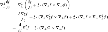 $$\begin{eqnarray}\displaystyle \unicode[STIX]{x1D6FB}_{\bot }^{2}\frac{\text{d}f}{\text{d}t} & = & \displaystyle \unicode[STIX]{x1D6FB}_{\bot }^{2}\left(\frac{\unicode[STIX]{x2202}f}{\unicode[STIX]{x2202}t}+\hat{z}\boldsymbol{\cdot }(\unicode[STIX]{x1D735}_{\bot }f\times \unicode[STIX]{x1D735}_{\bot }\unicode[STIX]{x1D719})\right)\nonumber\\ \displaystyle & = & \displaystyle \frac{\unicode[STIX]{x2202}\unicode[STIX]{x1D6FB}_{\bot }^{2}f}{\unicode[STIX]{x2202}z}+\hat{z}\boldsymbol{\cdot }(\unicode[STIX]{x1D735}_{\bot }\unicode[STIX]{x1D6FB}_{\bot }^{2}f\times \unicode[STIX]{x1D735}_{\bot }\unicode[STIX]{x1D719})+\hat{z}\boldsymbol{\cdot }(\unicode[STIX]{x1D735}_{\bot }f\times \unicode[STIX]{x1D735}_{\bot }\unicode[STIX]{x1D6FB}_{\bot }^{2}\unicode[STIX]{x1D719})\nonumber\\ \displaystyle & = & \displaystyle \frac{\text{d}}{\text{d}t}\unicode[STIX]{x1D6FB}_{\bot }^{2}f+\hat{z}\boldsymbol{\cdot }(\unicode[STIX]{x1D735}_{\bot }\unicode[STIX]{x1D6FA}\times \unicode[STIX]{x1D735}_{\bot }f).\end{eqnarray}$$
D.5 Commutator of
$\text{d}/\text{d}\ell$
and
$\unicode[STIX]{x2202}/\unicode[STIX]{x2202}t$


 $$\begin{eqnarray}\displaystyle \frac{\unicode[STIX]{x2202}}{\unicode[STIX]{x2202}t}\frac{\text{d}f}{\text{d}\ell } & = & \displaystyle \frac{\unicode[STIX]{x2202}}{\unicode[STIX]{x2202}z}\frac{\unicode[STIX]{x2202}f}{\unicode[STIX]{x2202}t}+\hat{z}\boldsymbol{\cdot }\left(\unicode[STIX]{x1D735}_{\bot }\frac{\unicode[STIX]{x2202}f}{\unicode[STIX]{x2202}t}\times \unicode[STIX]{x1D735}_{\bot }H\right)+\hat{z}\boldsymbol{\cdot }\left(\unicode[STIX]{x1D735}_{\bot }f\times \unicode[STIX]{x1D735}_{\bot }\frac{\unicode[STIX]{x2202}H}{\unicode[STIX]{x2202}t}\right)\nonumber\\ \displaystyle & = & \displaystyle \frac{\text{d}}{\text{d}\ell }\frac{\unicode[STIX]{x2202}f}{\unicode[STIX]{x2202}t}+\hat{z}\boldsymbol{\cdot }\left(\unicode[STIX]{x1D735}_{\bot }f\times \unicode[STIX]{x1D735}_{\bot }\frac{\unicode[STIX]{x2202}H}{\unicode[STIX]{x2202}t}\right).\end{eqnarray}$$
D.6 Commutator of
$\text{d}/\text{d}\ell$
and
$\text{d}/\text{d}t$


This derivation uses
 $$\begin{eqnarray}\displaystyle \frac{\text{d}\hat{z}\boldsymbol{\cdot }(\unicode[STIX]{x1D735}_{\bot }f\times \unicode[STIX]{x1D735}_{\bot }g)}{\text{d}\ell } & = & \displaystyle \hat{z}\boldsymbol{\cdot }\left(\unicode[STIX]{x1D735}_{\bot }\frac{\text{d}f}{\text{d}\ell }\times \unicode[STIX]{x1D735}_{\bot }g\right)+\hat{z}\boldsymbol{\cdot }\left(\unicode[STIX]{x1D735}_{\bot }f\times \unicode[STIX]{x1D735}_{\bot }\frac{\text{d}g}{\text{d}\ell }\right),\end{eqnarray}$$
which follows from the coordinate invariance of
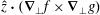 $\hat{z}\boldsymbol{\cdot }(\unicode[STIX]{x1D735}_{\bot }f\times \unicode[STIX]{x1D735}_{\bot }g)$
, equation (D 10).
$\hat{z}\boldsymbol{\cdot }(\unicode[STIX]{x1D735}_{\bot }f\times \unicode[STIX]{x1D735}_{\bot }g)$
, equation (D 10).
 $$\begin{eqnarray}\displaystyle \frac{\text{d}}{\text{d}\ell }\frac{\text{d}f}{\text{d}t} & = & \displaystyle \frac{\text{d}}{\text{d}\ell }\left(\frac{\unicode[STIX]{x2202}f}{\unicode[STIX]{x2202}t}+\hat{z}\boldsymbol{\cdot }(\unicode[STIX]{x1D735}_{\bot }f\times \unicode[STIX]{x1D735}_{\bot }\unicode[STIX]{x1D719})\right)\nonumber\\ \displaystyle & = & \displaystyle \left(\frac{\unicode[STIX]{x2202}}{\unicode[STIX]{x2202}t}\frac{\text{d}f}{\text{d}\ell }-\hat{z}\boldsymbol{\cdot }\left(\unicode[STIX]{x1D735}_{\bot }f\times \unicode[STIX]{x1D735}_{\bot }\frac{\unicode[STIX]{x2202}H}{\unicode[STIX]{x2202}t}\right)\!\right)+\frac{\text{d}}{\text{d}\ell }\hat{z}\boldsymbol{\cdot }(\unicode[STIX]{x1D735}_{\bot }f\times \unicode[STIX]{x1D735}_{\bot }\unicode[STIX]{x1D719})\nonumber\\ \displaystyle & = & \displaystyle \frac{\text{d}}{\text{d}t}\frac{\text{d}f}{\text{d}\ell }-\hat{z}\boldsymbol{\cdot }\left(\unicode[STIX]{x1D735}_{\bot }f\times \unicode[STIX]{x1D735}_{\bot }\left(\frac{\unicode[STIX]{x2202}H}{\unicode[STIX]{x2202}t}-\frac{\text{d}\unicode[STIX]{x1D719}}{\text{d}\ell }\right)\!\right)\nonumber\\ \displaystyle & = & \displaystyle \frac{\text{d}}{\text{d}t}\frac{\text{d}f}{\text{d}\ell }+\hat{z}\boldsymbol{\cdot }(\unicode[STIX]{x1D735}_{\bot }f\times \unicode[STIX]{x1D735}_{\bot }{\mathcal{N}}_{B}).\end{eqnarray}$$
D.7 Form of
$\hat{z}\boldsymbol{\cdot }(\unicode[STIX]{x1D735}_{\bot }f\times \unicode[STIX]{x1D735}_{\bot }g)$

 $$\begin{eqnarray}\hat{z}\boldsymbol{\cdot }(\unicode[STIX]{x1D735}_{\bot }f\times \unicode[STIX]{x1D735}_{\bot }g)=\frac{\unicode[STIX]{x2202}}{\unicode[STIX]{x2202}x}\left(f\frac{\unicode[STIX]{x2202}g}{\unicode[STIX]{x2202}y}\right)-\frac{\unicode[STIX]{x2202}}{\unicode[STIX]{x2202}y}\left(f\frac{\unicode[STIX]{x2202}g}{\unicode[STIX]{x2202}x}\right).\end{eqnarray}$$
D.8 Coordinate invariance of
$\hat{z}\boldsymbol{\cdot }(\unicode[STIX]{x1D735}_{\bot }f\times \unicode[STIX]{x1D735}_{\bot }g)$

In arbitrary coordinates
 $x_{a}(x,y)$
and
$x_{a}(x,y)$
and
 $y_{a}(x,y)$
, the gradient
$y_{a}(x,y)$
, the gradient
 $\unicode[STIX]{x1D735}_{\bot }f=(\unicode[STIX]{x2202}f/\unicode[STIX]{x2202}x_{a})\unicode[STIX]{x1D735}x_{a}+(\unicode[STIX]{x2202}f/\unicode[STIX]{x2202}y_{a})\unicode[STIX]{x1D735}y_{a}$
, which implies
$\unicode[STIX]{x1D735}_{\bot }f=(\unicode[STIX]{x2202}f/\unicode[STIX]{x2202}x_{a})\unicode[STIX]{x1D735}x_{a}+(\unicode[STIX]{x2202}f/\unicode[STIX]{x2202}y_{a})\unicode[STIX]{x1D735}y_{a}$
, which implies
 $$\begin{eqnarray}\displaystyle \hat{z}\boldsymbol{\cdot }(\unicode[STIX]{x1D735}_{\bot }f\times \unicode[STIX]{x1D735}_{\bot }g) & = & \displaystyle \frac{\unicode[STIX]{x2202}f}{\unicode[STIX]{x2202}x}\frac{\unicode[STIX]{x2202}g}{\unicode[STIX]{x2202}y}-\frac{\unicode[STIX]{x2202}f}{\unicode[STIX]{x2202}y}\frac{\unicode[STIX]{x2202}g}{\unicode[STIX]{x2202}x}\nonumber\\ \displaystyle & = & \displaystyle \displaystyle \left(\frac{\unicode[STIX]{x2202}f}{\unicode[STIX]{x2202}x_{a}}\frac{\unicode[STIX]{x2202}g}{\unicode[STIX]{x2202}y_{a}}-\frac{\unicode[STIX]{x2202}f}{\unicode[STIX]{x2202}y_{a}}\frac{\unicode[STIX]{x2202}g}{\unicode[STIX]{x2202}x_{a}}\right){\mathcal{J}}_{a};\end{eqnarray}$$
 $$\begin{eqnarray}\displaystyle {\mathcal{J}}_{a} & \equiv & \displaystyle \hat{z}\boldsymbol{\cdot }(\unicode[STIX]{x1D735}x_{a}\times \unicode[STIX]{x1D735}y_{a}).\end{eqnarray}$$
The Jacobian of the
 $(x_{a},y_{b})$
coordinates
$(x_{a},y_{b})$
coordinates
 ${\mathcal{J}}_{a}$
is unity when the coordinates are the starting points
${\mathcal{J}}_{a}$
is unity when the coordinates are the starting points
 $(x_{s},y_{s})$
of magnetic field line trajectories.
$(x_{s},y_{s})$
of magnetic field line trajectories.
