


I. INTRODUCTION
Multiple Input Multiple Output (MIMO) radars have received great interest over the last decade [Reference Bliss and Forsythe1, Reference Li and Stoica2] thanks to their potential compared with conventional radars. The essence of this concept is to probe simultaneously the channel with M orthogonal signals and record the backscattered signals with N receivers, which can spatially be independent to the transmitters. Thus, the received signal can be re-assigned to the source by performing correlation in pairs. This gives an enlarged virtual array improving the spatial resolution [Reference Bliss and Forsythe1]. The scattered signal of each couple of transmitter/receiver provides two main benefits: spatial diversity gain and increased degree-of-freedoms [Reference Wang3]. Each couple provides an information about the probed channel as shown in Fig. 1. The goal is to measure the scattering matrix (A) m,n which is given by:
 $$(A)_{m,n} \propto \int\!\int_{source} \displaystyle{1 \over {{(4\pi )}^2}}\displaystyle{{\exp ( - ik.r_{Tm})} \over {r_{Tm}}}\rho (r)\displaystyle{{\exp ( - ik.r_{Rn})} \over {r_{Rn}}}, $$
ρ(r) is the useful information referring to the reflectivity , r Tm and r Rn are the distance from respectively the transmitter m and the receiver n to the target (m ∈ [1, 2, …, M], n ∈ [1, 2, …, N]) as shown in Fig. 1. k is the wavenumber corresponding to the operation frequency.
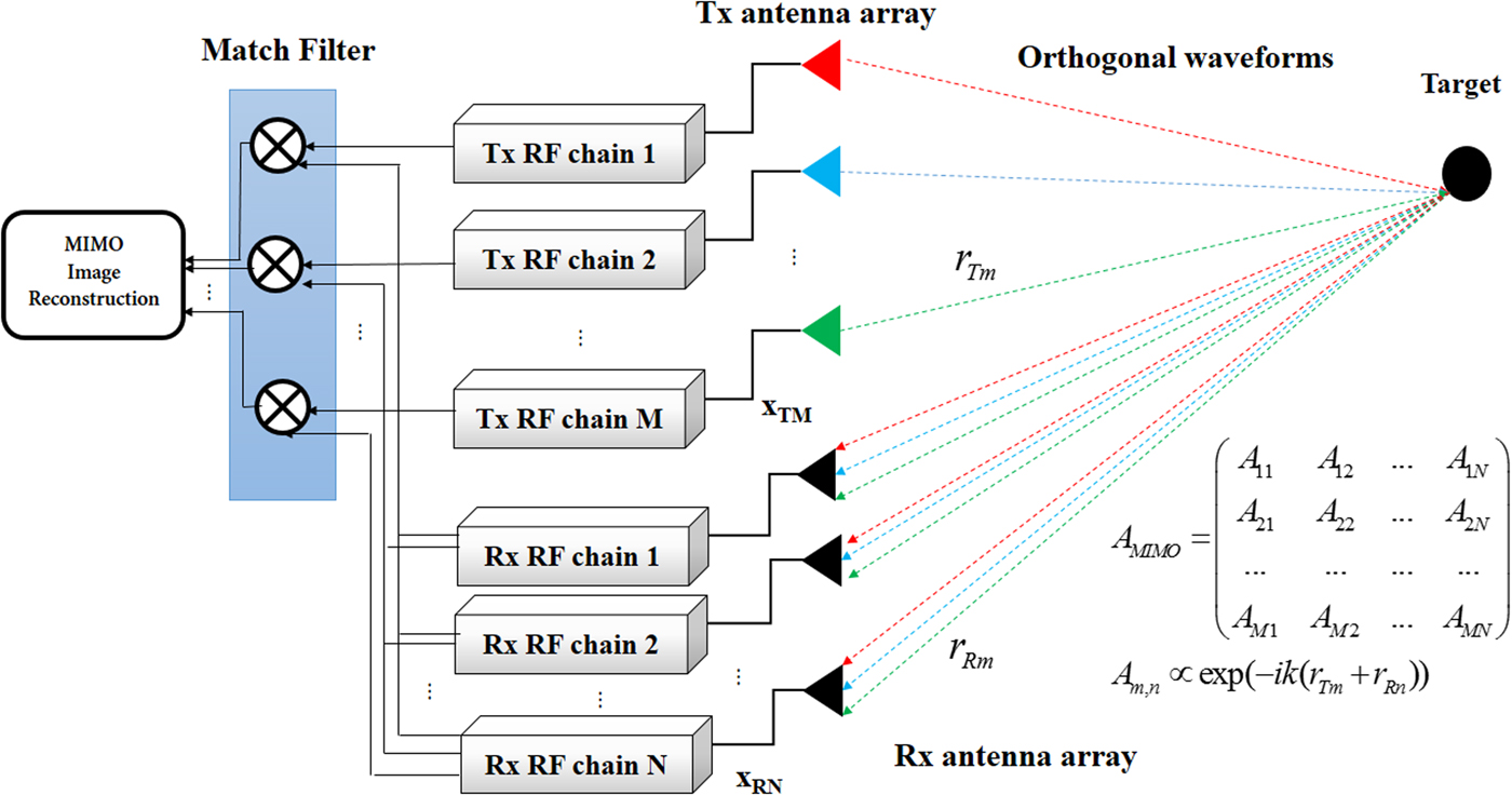
Fig. 1. Conventional MIMO Radar principle. The transmitted signals are orthogonal, thus the echo signals can be re-assigned to the source by performing correlation in pairs (A mn ). This gives an enlarged virtual receiver aperture improving the spatial resolution.
This scattering matrix can be sequentially measured by switching the transmitting antennas and jointly process the received signals [Reference Kpré, Fromenteze, Decroze and Carsenat4, Reference Kpré, Decroze, Carsenat and Fromenteze5]. To simultaneously probe the channel, the transmitted signals should be orthogonal. Therefore, it is obvious that the waveform design is an issue for a MIMO Radar systems.
Recent advances in MIMO Radar waveform design have spawned the publication of numerous papers. Deng [Reference Deng6] has initially proposed polyphase orthogonal code sets based on genetic algorithm. Space-time coding of linear frequency modulation has been proposed in [Reference Wang3–Reference Babur, Krasnov, Yarovoy and Aubry7] to mitigate cross-correlation effects in MIMO Radars, but the obtained waveforms are nearly orthogonal and need chirps de-ramping filters. A frequency hopping waveform is also an example of suitable that can be used for MIMO Radar. This waveform is chosen as the reference waveform for comparison with the proposed concept in this paper. The analytic formulation is as follows:
 $$s(t) = \sum\limits_{q = 0}^{Q - 1} u(t - qT_c).\exp (j2\pi (f_0 + c(q)\Delta f)t), $$
where:
 $$u(t) = \left( {\matrix{ {1,} & {{\rm if}\;0 \lt t \lt T_c.} \cr {0,} & {{\rm otherwise}.} \cr}} \right. ,$$
where f 0 is the center carrier frequency, c(q) is the qth element scrambled by a pseudo-noise Gold sequences [Reference Buehrer8], and Q, the number of carriers. T c corresponds to the pulse duration and is fixed by the total bandwidth B w of the signal. The echo signals can be re-assigned to the sources by performing correlation in pairs. The aim of the post-processing is first, to estimate the channel matrix A, which represents the interaction between the transmitting and receiving antennas, and then compensate the green functions to reconstruct the target signature. This is made possible by means of MIMO algorithms such as back-propagation of K-migration algorithm [Reference Chauvin and Rumelhart9, Reference Fromenteze, Kpre, Carsenat, Decroze and Sakamoto10]. The first one is the base of image reconstruction algorithm used in this paper.
All these aforementioned waveform design techniques are based on the conventional MIMO architecture, which should include M parallel transmitter chains ensuring Frequency up-conversion, Digital to analog conversion, etc. On the other hand, high resolution imaging will require as much RF chains as antennas needed in conventional MIMO architecture, which can rapidly be cumbersome and costly.
The contribution of this paper is to introduce an alternate pseudo-orthogonal waveform generation technique that requires a single transmitter radio frequency (RF) chain while maintaining the same transmitter antenna array. This is made possible by the means of a mode-mixing microwave cavity whose transfer functions are intrinsically uncorrelated [Reference Fromenteze, Kpre, Carsenat, Decroze and Sakamoto10–Reference Carsenat and Decroze16]. In this new approach, the orthogonality of the transmitted waveforms is passively ensured by the component transfer functions. As consequence, high orthogonality properties required in MIMO Radar Imaging can be achieved with a cost-efficient architecture.
The paper is organized as follows. Section II introduces the principle of unique Transmitter RF chain MIMO Radar and the mathematical formulations ensuing. The orthogonality metrics that should be met and numerical analysis are described in Section III. Experimental results are set forth in Section IV to show the effectiveness of the proposed method. Finally, a conclusion is drawn in Section V.
II. SINGLE TRANSMITTER RF CHAIN MIMO RADAR PRINCIPLE
Unlike a conventional MIMO architecture, the single-chain MIMO Radar needs a single transmitter RF chain to feed the required M transmit antennas. Since the transmitted signals toward the target should be orthogonal, the proposed architecture should satisfy this constraint. In practice, this constraint can be achieved by the mean of a microwave device whose transfer functions are uncorrelated [Reference Fromenteze, Decroze and Carsenat12]. As shown in Fig. 2, the transmit antennas are connected to a 1 × M passive microwave component, which can be an oversized microwave cavity [Reference Kpré, Fromenteze and Decroze13], a chaotic cavity, etc.
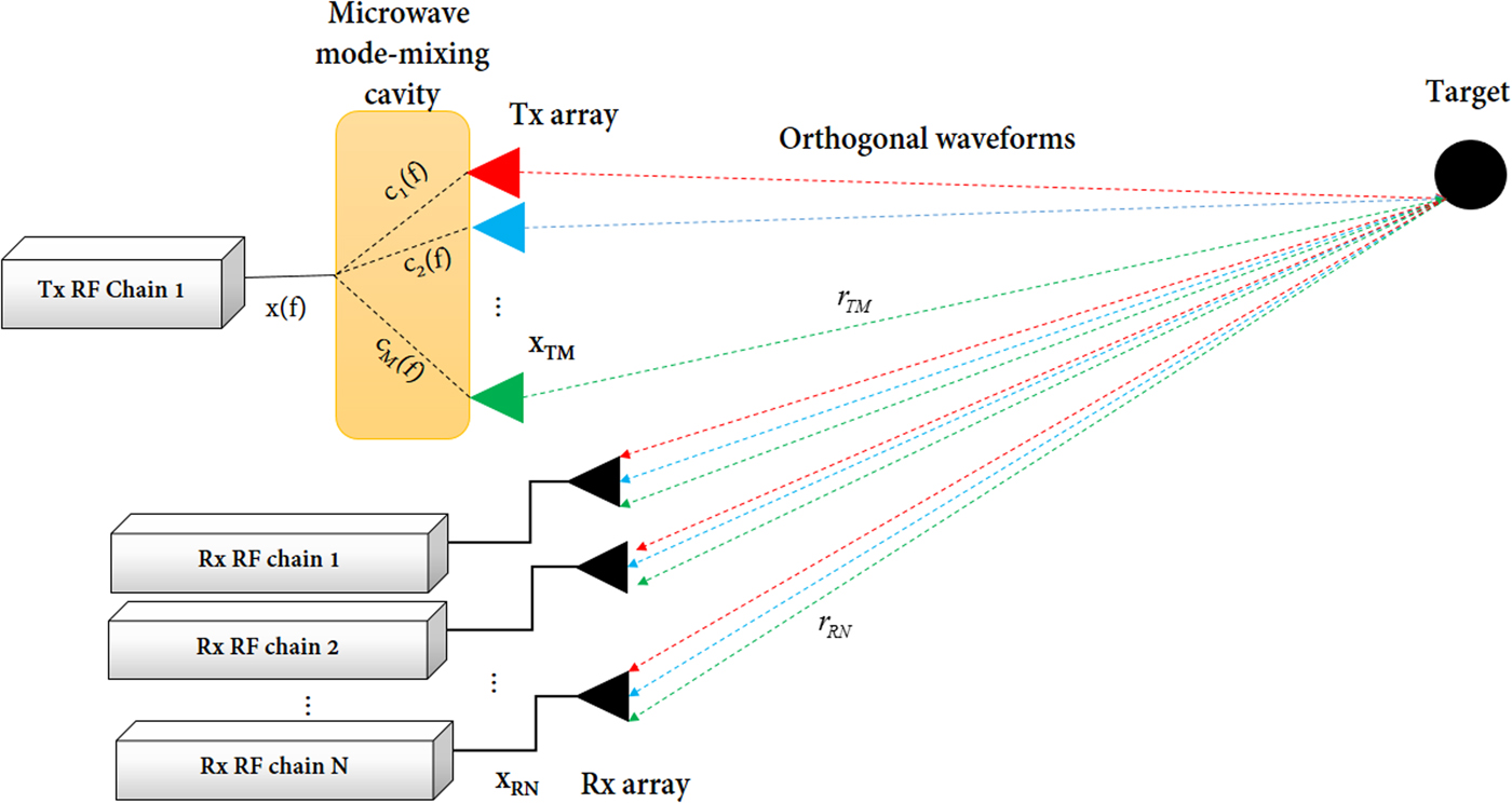
Fig. 2. Illustration of a single RF chain MIMO Radar transmitters fed by a 1 × M mode-mixing microwave cavity.
Indeed, an oversized microwave cavity relative to the propagating wavelength can reach a high modal density, which is necessary for good correlation properties. The time domain response of this kind of components can be modeled by the equation below [Reference Fromenteze, Kpre, Carsenat, Decroze and Sakamoto10–Reference Hill14]:
 $$c_m(t) = g_m(t).e^{ - t/2\tau _c}$$
where:
-
• gm (t) fits a zero-mean random Gaussian distribution. It can be seen as a Rayleigh multi-path channel. The channel richness depends on the size of the cavity compared with the propagating wavelength.
-
• τc corresponds to the channel delay spread (decay time), which is linked to the cavity quality factor. For an air-filled cavity, the quality factor depends essentially on the conductivity, and the number of input and output ports. Therefore, increasing the number of the transmitting antennas will decrease the quality factor, and thus impact the delay spread of each channel. This constraint should be considered while designing the cavity for MIMO Radar applications.
Furthermore, to improve frequency and spatial diversity inside the cavity, the number of degenerated modes can be minimized by means of a chaotic cavity. This can be achieved by a regular cavity with convex boundaries shape to obtain ergodic properties [Reference Lerosey15], or by inserting a diffusing object inside a regular cavity. In this paper, a simple regular oversized cavity is used to perform the experiment.
The first application of such cavities was introduced in [Reference Carsenat and Decroze16]. The authors demonstrated the ability to perform antenna beamforming without any electronically control using a 1 × 4 small regular reverberating chamber. Herein, this component is used as a passive chaotic waveform generator exploiting its intrinsic transfer function properties. In this context, a single waveform x(f) should be generated at the input of the component, and each transmitting antenna can be addressed independently with an orthogonal waveform at the output of the component. This allows the reduction of the number of transmitting RF chains compared with the conventional MIMO Radar architectures. In the depicted Fig. 2, the signal s m (f) radiated by the antenna m is :
 $$s_m(f) = x(f)c_m(f), $$
where x(f) is a unique signal generated at the input of the component, and c m (f) the component transfer function between the input and the mth output port of the component. For the sake of notation simplicity, equation (5) can be presented in linear equation form, with an implicit notation of the frequency:
 $${\bf s} = x\;{\bf c}. $$
Note that vectors and Matrix are respectively, represented by a bold and capital bold character. Therefore, the signals measured by the receiving antenna array considering a noiseless scenario is:
 $${\bf y} = {\bf As}, $$
with A the aforesaid scattering matrix, which accounts for useful information required for the imaging. An estimated ${\bf A}_r$
of the channel matrix can be computed for each frequency by compensating the contribution of the generated waveform x and the component transfer functions c in a single operation:
${\bf A}_r$
of the channel matrix can be computed for each frequency by compensating the contribution of the generated waveform x and the component transfer functions c in a single operation:
 $${\bf A}_r = {\bf y}{\bf s}^ +, $$
where ${\bf s}^ + $
is the transmitted waveform equalizer. Numerous equalization techniques can be applied to solve this linear problem, Tikhonov approach is an example of suitable methods to solve it. The explicit solution is thus given by [Reference Klema and Laub17]:
${\bf s}^ + $
is the transmitted waveform equalizer. Numerous equalization techniques can be applied to solve this linear problem, Tikhonov approach is an example of suitable methods to solve it. The explicit solution is thus given by [Reference Klema and Laub17]:
 $${\bf s}_\mu ^ + = ({\bf s}^\dagger {\bf s} + \mu I)^{ - 1}{\bf s}^\dagger , $$
where μ denotes the regularization parameter, which is used as a threshold to prevent any ill-conditioning problem [Reference Fromenteze, Decroze and Carsenat12]. $(.)^\dagger $
denotes the transposed-conjugate operator. The expression of the estimated channel matrix can be expressed by:
$(.)^\dagger $
denotes the transposed-conjugate operator. The expression of the estimated channel matrix can be expressed by:
 $$\eqalign{{\bf A}_r &= {\bf ys}_\mu ^ + \cr &= {\bf Ass}_\mu ^ + \cr &\approx {\bf A}{\bf R}_\mu}.$$
Considering an ideal equalization of the generated signal x at the device input, ${\bf R}_\mu $
can be considered as the pseudo-correlation matrix of the component transfer functions:
${\bf R}_\mu $
can be considered as the pseudo-correlation matrix of the component transfer functions:
 $${\bf R}_\mu = \left[ {\matrix{ \hfill {c_1 \times c_{1\mu} ^ +} & \hfill {c_1 \times c_{2\mu} ^ +} & \hfill \ldots & \hfill {c_1 \times c_{m\mu} ^ +} \cr \hfill {c_2 \times c_{1\mu} ^ +} & \hfill {c_2 \times c_{2\mu} ^ +} & \hfill \ldots & \hfill {c_2 \times c_{m\mu} ^ +} \cr \hfill \ldots & \hfill \ldots & \hfill \ldots & \hfill \ldots \cr \hfill {c_m \times c_{1\mu} ^ +} & \hfill {c_m \times c_{2\mu} ^ +} & \hfill \ldots & \hfill {c_m \times c_{m\mu} ^ +} \cr}} \right].$$
Ideally, this matrix tends to an identity matrix, corresponding to uncorrelated transfer functions leading to a perfect estimation of the channel matrix ${\bf A}_r \approx {\bf A}$
. Such constraints are not practically achievable, limited by the frequency diversity of microwave components, but can be approached using an oversized microwave cavity regarding the operating wavelength [Reference Kildal and Rosengren18].
${\bf A}_r \approx {\bf A}$
. Such constraints are not practically achievable, limited by the frequency diversity of microwave components, but can be approached using an oversized microwave cavity regarding the operating wavelength [Reference Kildal and Rosengren18].
III. ORTHOGONALITY METRICS
A) Correlation criterion
For MIMO radar applications, the probing signals must have good correlation properties : thin autocorrelation pick and low cross-correlation sidelobes to minimize interferences between channels. The cross-correlation function between two signals generated from two different antennas (i.e. s i (t) and s j (t), (i, j) ∈ [1, 2, …M])must satisfy the condition below :
 $$\eqalign{r_{ij}(t) = & s_i(t) \otimes s_j(t) \cr = & \int_{ - \infty} ^\infty s_i(t).s_j^* (t - \tau )dt = 0\quad \forall i \ne j}, $$
where (.)* denotes complex conjugate of the argument (.). For an infinite bandwidth, r ii (t) tends to a Dirac function δ(t).
An important metric to evaluate this correlation property is the Person correlation coefficient (PCC), which is defined by [Reference Pearson19] :
 $$\rho (i,j) = \displaystyle{{cov[s_i(t)s_j(t)]} \over {\sigma _i\sigma _j}} ,$$
where cov[s i (t)s j (t)] is the covariance between s i (t) and s j (t), and σ i and σ j are the standard deviation of the s i (t) and s j (t), respectively. The PCC gives an indication of the linear relationship between the two signals. If ρ(i, j) = 0, then s i (t) and s j (t) are said uncorrelated. Whereas, the closer the value of ρ(i, j) is to 1 the stronger the correlation between the two signals. Figure 3 shows an example of an oversized air-filled microwave cavity with outer dimensions of 0.8 × 0.8 × 1 m3. The component is constituted of 1 × 24 (Input/Output) ports. The transfer functions have been characterized and the correlation coefficients have been computed for 16 channels. As it can be noticed in Fig. 3(e) the device transfer functions are uncorrelated. As result, it can be utilized to generate pseudo-orthogonal waveform for MIMO Radar applications.

Fig. 3. Example of an oversized microwave cavity. (a) The front side of the cavity with output ports. (b) Inner-view with UWB probes randomly placed inside the empty cavity. (c) The backside of the cavity with a single input port. (d) The transfer function between the input port and output port 1. (e) Correlation coefficients of 16 transfer functions.
B) Conditioning criterion
An other metric to evaluate the performances of the proposed concept is the condition number, which helps to evaluate the impact of errors on the scattering matrix reconstruction. Let us consider a MIMO array of M transmitters and N receivers. As mentioned in equation (7), the received signal vector can be given in the frequency domain by the equation y = As leading to a corresponding solution ${\bf A}_{\bf r} = {\bf y}{\bf s}^ + $
. Thereby, an error in y will unfortunately beget a wrong estimation of the scattering matrix.
${\bf A}_{\bf r} = {\bf y}{\bf s}^ + $
. Thereby, an error in y will unfortunately beget a wrong estimation of the scattering matrix.
The condition number gives a bound on how inaccurate the solution ${\bf A}_{\bf r}$
will be after equalization. It can be seen as the rate at which the solution will change with respect to a change in y. Assuming an error ε in y, the error in the solution is
${\bf A}_{\bf r}$
will be after equalization. It can be seen as the rate at which the solution will change with respect to a change in y. Assuming an error ε in y, the error in the solution is ${\epsilon}. {\bf s}^ + $
. Thus,the ratio of the relative error in
${\epsilon}. {\bf s}^ + $
. Thus,the ratio of the relative error in ${\bf A}_{\bf r}$
and y can be expressed as follows [Reference Belsley, Kuh and Welsch20]:
${\bf A}_{\bf r}$
and y can be expressed as follows [Reference Belsley, Kuh and Welsch20]:
 $$ERR = \displaystyle{{ \vert \vert {\epsilon}. {\bf s}^ + \vert \vert / \vert \vert {\bf y}{\bf s}^ + \vert \vert} \over { \vert \vert {\epsilon} \vert \vert / \vert \vert {\bf y} \vert \vert}} = \left( {\displaystyle{{ \vert \vert {\epsilon}. {\bf s}^ + \vert \vert} \over { \vert \vert {\epsilon} \vert \vert}}} \right)\left( {\displaystyle{{ \vert \vert {\bf y} \vert \vert} \over { \vert \vert {\bf y}{\bf s}^ + \vert \vert}}} \right) ,$$
for non-zeros y and ε, the maximum value is bounded by the product of the two operator norms:
 $$\eqalign{ER_{max} = & {\rm ma}{\rm x}_{({\epsilon}, {\bf y} \ne 0)}\left( {\displaystyle{{ \vert \vert {\epsilon}. {\bf s}^ + \vert \vert} \over { \vert \vert {\epsilon} \vert \vert}}} \right)\left( {\displaystyle{{ \vert \vert {\bf y} \vert \vert} \over { \vert \vert {\bf y}{\bf s}^ + \vert \vert}}} \right) \cr = & \left( {{\rm ma}{\rm x}_{({\epsilon} \ne 0)}\displaystyle{{ \vert \vert {\epsilon}. {\bf s}^ + \vert \vert} \over { \vert \vert {\epsilon} \vert \vert}}} \right)\left( {{\rm ma}{\rm x}_{({\bf y} \ne 0)}\displaystyle{{ \vert \vert {\bf y} \vert \vert} \over { \vert \vert {\bf y}s^ + \vert \vert}}} \right) \cr = & \left( {{\rm ma}{\rm x}_{({\epsilon} \ne 0)}\displaystyle{{ \vert \vert {\epsilon}. {\bf s}^ + \vert \vert} \over { \vert \vert {\epsilon} \vert \vert}}} \right)\left( {{\rm ma}{\rm x}_{(\forall {\bf v} \ne 0)}\displaystyle{{ \vert \vert {\bf v}s \vert \vert} \over { \vert \vert {\bf v} \vert \vert}}} \right) \cr = & \vert \vert {\bf s}^ + \vert \vert. \vert \vert {\bf s} \vert \vert}, $$
finally the condition number $\kappa ({\bf s})$
can be bounded by :
$\kappa ({\bf s})$
can be bounded by :
 $$\kappa ({\bf s}) = \vert \vert {\bf s}^ + \vert \vert. \vert \vert {\bf s} \vert \vert \ge \vert \vert {\bf s}^ + {\bf s} \vert \vert = 1. $$
Therefore, if the condition number is large, even a small error ε may occur large error in the scattering matrix. On the other hand, smaller error in y will not produce much error in ${\bf A}_{\bf r}$
. Furthermore, when
${\bf A}_{\bf r}$
. Furthermore, when $\kappa ({\bf s})$
is exactly one, then the equalization operation defined by equation (8) can find an approximation solution
$\kappa ({\bf s})$
is exactly one, then the equalization operation defined by equation (8) can find an approximation solution ${\bf A}_r$
, which is very close to the real scattering matrix A. As consequence, a signal s with condition number nearby 1 is said well-conditioned, and that with infinite condition number is said ill-conditioned (this implies that equation (7) does not possess a unique, and well-defined solution).
${\bf A}_r$
, which is very close to the real scattering matrix A. As consequence, a signal s with condition number nearby 1 is said well-conditioned, and that with infinite condition number is said ill-conditioned (this implies that equation (7) does not possess a unique, and well-defined solution).
Figure 4 show a comparison between a conventional orthogonal frequency waveform of Q = 32 carriers with the orthogonal waveforms generated by an oversized cavity. For this comparison, the frequency range is set from 2.5 to 3.5 GHz. The component decay time was set to 500 ns and 16 waveforms are considered.
Fig. 4. Comparison of the conditioning number of a conventional orthogonal frequency hopping waveform and the mode-mixing waveform.
Noticeably, the frequency hopping waveform is well-conditioned compared with the mode-mixing waveform, which implies a better reconstruction of the scattering matrix. That is due to the fact that the frequency hopping can be well controlled. While, the microwave cavity considered here is an entirely passive component, and the conditioning belongs to its intrinsic properties. Increasing the signal bandwidth will increase the number of modes inside the cavity providing more frequency diversities. As a consequence, the conditioning number is minimized. Minimizing the number of degenerated modes can certainly be helpful to improve the conditioning number.
IV. MEASUREMENT RESULTS
In this section, a measurement bench is set up to show the feasibility of the proposed method. The air-filled microwave aforementioned is used to connect M = 4 transmit antennas. The N = 4 receivers are directly connected to an oscilloscope Agilent DSO90404A 20 GSa/s. The inter-elements spacing is dT = 1.4 × λ c and dR = 0.7 × λ c respectively, the transmitting and the receiving antennas. λ c corresponds to the central wavelength in the 2.5–3.5 GHz frequency Bandwidth. First, a conventional MIMO radar measurement is performed by the mean of four orthogonal frequency hopping waveforms generated by a four channels Arbitrary waveform generator Agilent M8190A 12 GSa/s. Then the same radar scenario was made by the mean of the proposed method. Figure 5 shows the measurement setup.
Fig. 5. MIMO Radar measurement setup. (a) Conventional MIMO with four FH-waveforms generated by an arbitrary waveform generator (AWG). (b) Mode-mixing MIMO measurement setup, the transmitters are connected to the metallic cavity behind and the receivers are connected to a digital oscilloscope.
Fig. 6. MIMO radar imaging results. (a) A metallic cylinder with isotropic radar cross-section. (b) and (c) are respectively, the cylinder imaging result with the FH and the mode-mixing waveform. (d) Two metallic ribbons placed in front of the radar. (e) and (f), the imaging result of the two water bottles.
The backscattered signals are measured and the same post-processing and MIMO back-propagation algorithm [Reference Chauvin and Rumelhart9] is applied to both methods to locate the targets. Figure 5 show the imaging results, which uphold the feasibility of the proposed method. With a single generated waveform at the microwave device input, the MIMO channel matrix can be measured in one shot. The beam width at –3 dB of the maximum is about 8° for both methods. For the mode-mixing waveform, the image Peak-to-noise Ratio is about 14.27 and 12.76 dB respectively, the cylinder and the two metallic ribbons image while those of the conventional FH-MIMO are about 16.21 and 13.83 dB. As it can be noticed, the target can clearly be located with a single transmit RF chain ensuring MIMO Radar architecture simplification with respect to the transmit beamforming constraint.
V. CONCLUSION
This paper is assessed in more detail the orthogonality metrics of the mode-mixing waveform, as previously studied. Using a passive microwave component whose transfer functions are quasi-orthogonal, MIMO radar transmitters can be independently addressed via a single generated waveform at the device input port. This condition has been achieved by means of an oversized microwave cavity regarding the operating wavelengths. The measurement results show that the proposed method can be applied to minimize the complexity of the conventional MIMO Radar architecture. Only a single transmitter RF chain is required to feed the same antenna array. Future works will focus on the design of miniaturized microwave components that can provide good correlation properties, accurate algorithms will be developed to enhance the image reconstruction.
 Ettien Lazare Kpré received the M.S. degree in microwave engineering from Limoges University, in 2014. He is currently a Ph.D. researcher with the Xlim Research Institute. His main research interests include signal processing, MIMO radar, passive microwave devices, Synthetic Aperture Interferometric Radiometer, and Microwave imaging.
 Cyril Decroze received the Ph.D. degree in telecommunications engineering from the University of Limoges, Limoges, France, in 2002. He is currently an Associate Professor with the XLIM Research Institute, University of Limoges. Since 2006, he has been in charge of the wireless systems activity with the Wave and Associated System Department, XLIM Research Institute. His field of research concerns multiple-antennas systems and associated processing for telecommunications and radar imaging.
 Thomas Fromenteze received the Ph.D. degree from the University of Limoges, France, in 2015. He is currently a Post-Doctoral Researcher with the CMIP, Duke University, USA. His main research interests lie in ultrawideband microwave imaging, wave propagation in complex media, and the associated inverse problems. He received the 11th EuRAD Young Engineer Prize during the European MicrowaveWeek 2015.


