1. INTRODUCTION
Tomiyama et al. (Reference Tomiyama, Beek, Cabrera, Komto and Hitoshi D'Amelio2013) provide a solid analysis of the reasons behind the important gap that exists between the study and usage of function modeling in academia and among industrial practitioners. The concept of a function can be used for several purposes within the engineering design process. It is, for example, used in requirements engineering. Requirements templates such as boilerplates (Dwyer et al., Reference Dwyer, Avrunin and Corbett1999) are often formed using simple subject–verb–noun triplets. Requirements do not exclusively represent functions, but a great part of them are functional requirements (to do something). The function is a classical way to describe the overall purpose of a system, to describe the internal structure, architecture, and behavior of a system. Different aspects of function thinking or modeling have already been used and taught for a long time as an important part of the engineering design process (Pugh, Reference Pugh1991; Otto & Wood, Reference Otto and Wood2001; Pahl & Beitz, Reference Pahl and Beitz2013). For example, for development phases and tools in requirements engineering to describe the functional requirements, quality function deployment to allocate customer needs to functions, system engineering to represent the system architecture, and also for system development management purposes, value engineering (Miles, Reference Miles1967). Therefore, why, despite its presence all over the engineering design process, is function modeling not more widely used by design practitioners in several of the design and engineering communities? Several reasons exist that can explain the limited usage of function modeling in industry (Tomiyama et al., Reference Tomiyama, Gu, Jin, Lutters, Kind and Kimura2009, Reference Tomiyama, Beek, Cabrera, Komto and Hitoshi D'Amelio2013). First, the engineering academic community, which is trying to promote function modeling, often presents studies related to new product development, even though most of the design activities inside companies are routine or incremental design tasks. The academic community seldom studies incremental or routine design tasks. Consequently, practitioners often consider that their everyday activities cannot be supported by function modeling. Tomiyama et al. refer to this as a “not practical” syndrome among practitioners (Tomiyama et al., 2009, Reference Tomiyama, Beek, Cabrera, Komto and Hitoshi D'Amelio2013). Second, the added value of function modeling is often not immediately perceived by practitioners. It is often considered more efficient and more immediately rewarding to represent a solution quickly in a three-dimensional computer-aided design software tool, instead of taking time to abstract the solution in the form of a function model. In addition, function models, when developed, can quickly explode and become difficult to manage; function modeling is often seen as a source of wasted time. Third, there are few professional software tools capable of representing big function models efficiently on a computer screen of limited size. It is particularly difficult to get an overall picture of a complex function model on a computer screen. Another element limiting the impact of function analysis is the abstraction gap that exists between function models and design structures. In the literature, several models have been proposed to bridge this gap. The function–behavior–structure (FBS models; Gero, Reference Gero1990) and the requirement–function–behavior–structure model (Christophe et al., Reference Christophe, Bernard and Coatanéa2010) are both attempts to connect functions to behaviors, states, and structures. Nevertheless, those models provide little operational support for function-level or qualitative simulation of system behaviors (Tomiyama et al., Reference Tomiyama, Beek, Cabrera, Komto and Hitoshi D'Amelio2013). The qualitative simulation should improve the product development process (Sen & Summers, Reference Sen and Summers2013; Tomiyama et al., Reference Tomiyama, Beek, Cabrera, Komto and Hitoshi D'Amelio2013).
The present article proposes to integrate function modeling into a broader framework to achieve three concrete goals: first, to support the representation of physics-based reasoning; second, to use this physics-based reasoning to assess design options; and third, to use the framework to support innovative ideation. In this article, the exemplification of the functional-based approach is performed via the use of a case study proposed for this special issue: a glue gun. A reverse engineering approach is applied, and the authors seek an incremental improvement of the solution. The approach follows an iterative process to break the functions down from a black box model to a functional model with the desired level of detail. The approach aims at converting the function models to a list of governing equations and a causal graph between the variables in the system.
The rest of this paper is organized as follows: a state-of-the-art analysis of the concept of functions and of different functional techniques is presented in Section 2. This section ends with a description of the approaches that can be used to limit the variability of function modeling. In Section 3 and Section 4, the successive modeling steps and theoretical aspects of the dimensional analysis conceptual modeling (DACM) framework are presented. This is followed by the case study in Section 5, in which DACM framework modeling is applied to model the glue gun, to illustrate the several different modeling options, and to demonstrate the added value of the framework. In the discussion/conclusion Section 6, the capabilities, current limitations, and future developments of the DACM framework are discussed further.
2. BACKGROUND
2.1. Nature of functions in different methodologies and theories
To introduce the concept of functions, the definition of an artificial system proposed by Le Moigne is relevant. According to Le Moigne (Reference Le Moigne1994), influenced by Von Bertalanffy and other systems theorists, a general system is an artifact (i.e., an artificial object) evolving in a certain environment to fulfill a purpose (i.e., a finality). This artifact functions (i.e., does activities) and its internal structure evolves over time, without losing its structure. Artifact or natural systems do activities. Consequently, they exhibit functions. These functions are an abstract concept describing the activities of a system. The concept of a function is present in sciences such as biology (Dusenbery, Reference Dusenbery1992), economics (Stahel, Reference Stahel1997), and systems theory (Le Moigne, Reference Le Moigne1994; Luhmann, Reference Luhmann2013). The concept is extremely useful in analyzing complex systems. To quote from Herbert Simon (Reference Simon1996): “We define a polar bear by the conjunction of a project: survive by functioning, an environment: The Arctic continent, then by analysing the structural anatomy of this bear… .”
The importance attributed by systems theory and systems engineering to the concept of a function is also present in engineering design. Nevertheless, the concrete usage made of the concept depends greatly on the authors and the viewpoints they adopt. In the work of Pahl and Beitz (Reference Pahl and Beitz2013), a functional structure is defined as “a meaningful and compatible combination of sub-functions into an overall function.” The functions are classified as main and auxiliary functions. Main functions are those subfunctions that serve the overall function directly, and auxiliary functions are those that contribute to it indirectly. The definition of a function and the relations between functions and design parameters are general, and the final decision about the meaningful and compatible combination of the function depends uniquely on the designer's personal preference. In axiomatic design (Suh, Reference Suh1990), functional requirements are defined as “the minimum set of independent requirements that completely characterize the design objective for a specific need.” The concept of a function is still fuzzy, and no distinction between main and auxiliary functions is made by the author. In the initial general design theory in 1981, Yoshikawa defines a function thus: “When an entity is exposed to a circumstance, a peculiar behavior appears corresponding to the circumstance. This behavior is called a visible function. Different behaviors are observed for different circumstances. The total of these behaviors is called a latent function. Both are called function inclusively” (Yoshikawa, Reference Yoshikawa, Sata and Warman1981). In the NFX50-151 standard (NFX50-151, 1991), a function is defined as “an action of a product or one of its components expressed in terms of finality.” The standard also distinguishes two types of functions. The first one is called a service function. The service function is “the actions expected of the product in order to answer the user's needs.” The second type of function is a constraint function, which is the “limitation of the designer's freedom considered to be necessary for the applicant.”
In most of the design methodologies or theories, the arguments about functions are not intended to give a clear definition of the function itself, but to show how desired overall functions are decomposed into identifiable subfunctions until they correspond to certain entities or design objects. Often implicitly (and in disagreement with principles from value analysis or system engineering), the designer has a solution in mind and maps this solution with a function decomposition matching this representation. This aspect often remains implicit and is rarely studied in functional analysis. In particular, when incremental innovation or routine design tasks are taking place, a functional model is the result of an iterative process that ends when the functional model matches the physical solution. This interplay between function/structure–behavior requires further research. Functions are usually used in two ways, for analyzing an existing object by discovering “How does this object function?” or to design a new service or artifact by answering the question “What are the artifact's functions?” In other terms, function modeling can be used to perform reverse engineering analysis, as per its main use in Otto and Wood (Reference Otto and Wood2001) or to create new artifacts. The nature of the day-to-day design activity characterized by routine or incremental design tasks is better grasped by answering the question “How does this object function?” and by performing reverse engineering. The question nevertheless remains of “How is value for the designer to be generated with the reverse engineering approach?” There is a need for a methodology based on reverse engineering and capable of analyzing the weaknesses of existing solutions but also exploring the design space and evaluating the potential design directions. The concept of value is addressed in the DACM framework developed in the article. The selection of colors for the causal graphs in DACM is a way to represent the values and viewpoints of the designers.
Currently, function modeling offers few methods to provide solid support to those objectives. The methods briefly presented above allow the gap between functions on one side and structure and behavior on the other side to be bridged to some extent but are not capable of providing simulation capabilities and especially capabilities to support physics-based reasoning to assess design options and for ideation purposes. A fundamental paradox emerges. Function modeling is an attempt to abstract and formalize design problems in order to understand the nature of the problem better, but at the same time, there is a need for early concretization and validation via prototyping and/or simulation. How can this be done quickly and easily in early stages without the need for complex prototyping or simulations? The article aims to reconcile these viewpoints by associating function models and early simulations.
Functions are used at different stages of the design process for different purposes. Specific processes and tools reflecting the different viewpoints and usages have been developed. This section provides a rapid overview of the most common processes and function representations. In systems engineering (INCOSE, 2012; System Engineering Fundamentals, 2013), a specific effort is made to identify the functional requirements, to decompose them to lower function levels, to allocate performances and limitations to the different functional levels, to define functional interfaces, to develop functional architectures, and to transform functional architectures into physical architectures. Figure 1 illustrates this rich usage of functions in systems engineering.

Fig. 1. Design process in the IEEE 1220 Standard (IEEE, 2005).
Figure 2 presents the different steps of the systems engineering process where the concept of functions is used. The functionalities of a system are considered throughout the life cycle of a design project. On the contrary, the functional modeling occurs only at the beginning of a development process. At this early stage too, verification is needed, and instead of considering the development process as a single V model (VDI, 1993), it might be more appropriate to consider multiple imbricated V cycles where verifications take place at each stage of the process. This article aims to provide such a type of verification capability for function modeling. Figure 3 summarizes a few of the most common forms used for the decomposition of a function or functional architecture, such as the functional tree, the functional structure, and the coupling matrix (NFX50-151, 1991; Le Moigne, Reference Le Moigne1994). The functional structure is the most commonly used.

Fig. 2. The systems engineering process (Systems Engineering Fundamentals, 2013).

Fig. 3. Different functional representations.
The functional boxes themselves can be depicted using three colors to characterize the level of knowledge associated with those boxes. Figure 4 presents those colors. The inputs and outputs of the functional boxes also have different forms. The representation from Pahl and Beitz shown in Figure 5 is the most commonly used.

Fig. 4. The color code used in the standard IEEE 1220 Standard (IEEE, 2005) to represent a system.

Fig. 5. Inputs and outputs in functional boxes.
Another way to represent a function is the octopus diagram in Figure 6. The diagram presents the different elements of the environment and the system to be designed. The diagram allows the listing of the different service functions of systems, as well as the constraint functions. It can also be replaced in the system modeling language using a use case diagram (Friedenthal et al., Reference Friedenthal, Moore and Steiner2008).

Fig. 6. Functional representation using an octopus diagram (de la Bretesche, Reference de la Bretesche2000).
A design structure matrix (DSM) is a way of representing a graph but also a functional architecture. A good overview of DSM usage is provided by (Eppinger & Browning, Reference Eppinger and Browning2012). A DSM is especially used to model the structure of systems or processes. A DSM lists all the constituent parts of a system or the activities of a process and the corresponding information exchange, interactions, or dependency patterns. DSMs compare the interactions between elements of a similar nature. Figure 7 presents an example of a DSM used to map functions together. A DSM is a square matrix (i.e., it has the same number of columns and lines) that maps elements of the same domain. A domain mapping matrix associates elements of a different nature in a matrix format and can also be used to map, for example, functions and components. The DACM framework presented in Section 3 utilizes DSM as an efficient way to automatize the physics-based reasoning approach.

Fig. 7. Example of a simple design structure matrix (function to function mapping).
The architecture of a system is usually represented using the functional structure or a rich representation language such as Integrated Definition Methodology (IDEF; Hanrahan, Reference Hanrahan1995) or one of the diagrams from system modeling language (Friedenthal et al., Reference Friedenthal, Moore and Steiner2008), such as an activity diagram or a sequence diagram. Through all its variants the IDEF representation language allows multiple aspects of functions to be represented. The sequence of functions can also be represented using languages such as Petri nets or Grafcet (NFC03-190+R1, 1995). Figure 8 represents the two-function modeling of a hybrid vehicle. In the hybrid series architecture, only electrical energy is used to generate the final mechanical energy required for the wheels, while in the parallel architecture both mechanical and electrical energy can be used simultaneously. Each of those powertrain configurations offers specific advantages. The parallel configuration can generate more instant power, while the series architecture is more fuel efficient.

Fig. 8. Two functional architectures of a hybrid vehicle.
Functional modes existing in complex systems can also be represented via a hybrid representation model such as that presented in Figure 9. These modes each represent the activations of different functions in a single-function model of a hybrid vehicle. This presentation is not exhaustive, but the aim was to present the richness of the functional description where multiple modes of functional representations have been developed over time. As a summary of this description, the usage of functions within design methods as a concept and as a design technique representation varies significantly. In general, the literature related to complex systems advises making intensive use of function modeling (Hmelo-Silver et al., Reference Hmelo-Silver, Rebecca, Liu, Gray, Demeter, Rugaber, Vattam and Goel2008). On the contrary, the field of product development and design thinking (Bowler, Reference Bowler1976; Rowe, Reference Rowe1991) seldom refers to the concept of functions, probably because of the scope of the problems tackled by those approaches. This significant difference between systems engineering and design thinking is a source of a major question for the authors of this article. Tension exists between the need to abstract and the parallel need to prototype. Prototyping seems more rewarding for designers than abstracting. In particular, the benefit of physical prototypes is immediately visible and provides a feeling of concrete achievement. This impression of achievement is also present with digital prototypes.

Fig. 9. Six functioning modes of a hybrid vehicle.
2.2. Physics-based reasoning in function modeling
The early stages of designing a product usually involve the activity of proposing a variety of possible solutions to satisfy the design requirements. The designer might analyze the feasibility of the initial solutions. He might consider the trade-offs and select one solution among the variety of possible solutions. He might analyze how changing a design parameter affects the overall performance of a proposed solution. Therefore, the selection of one from among the possible existing solutions is very dependent on the experience of the designer of providing rationales. In order to enhance such analysis in the early stage of design, one possible direction is to enable physics-based reasoning on function models. In his dissertation Sen (Reference Sen2011) stated that a function-based representation is suitable for supporting early design analysis reasoning. Sen and Summers (Reference Sen and Summers2013) identified requirements to enable physics-based reasoning from a function model. They extracted the following requirements:
-
1. Coverage: This is the ability to cover the knowledge and principles of various domains and their interactions, such as electrical, mechanical, thermal, and chemical engineering.
-
2. Consistency: Consistency is an internal property in the representation to prevent internal conflict.
-
3. Validity against the laws of physics: The function model representation should remain valid against the existing laws of physics in each domain.
-
4. Physics-based concreteness: The functions should be defined in terms of physical actions.
-
5. Normative and descriptive modeling: The representation should support both developing a function model for new product design (so-called normative modeling) and the function modeling of an existing artifact, concepts, or physical principles (so-called descriptive modeling).
-
6. Qualitative modeling and reasoning: It must enable support for both qualitative and quantitative reasoning.
The first three requirements were stated to be generic requirements, and the others are based on their study of identified gaps in function-based design (Summers & Shah, Reference Summers and Shah2004). Those requirements were taken into account in developing the DACM framework and user interface.
2.3. Variability in function modeling, DACM scope, and relevant approaches in literature
The function modeling process is a source of great variability, which can be caused by multiple factors, such as the modeler's preferences and experience, for example, the functional vocabulary used by the modelers, the level of abstraction, and the level of detail selected. Variability can also exist at the functional architecture level. Variability as such is not a source of problems if the goal is to generate a large number of solutions. These sources of variability can be a source of creativity during the early stages during the divergent thinking process. Nevertheless, when repeatability in the models is required in order to communicate function modeling without ambiguity, the variability of function modeling is a source of problems for the modelers and for any physics-based reasoning analysis.
A mechanism ensuring convergence in the modeling process is required in this work if we want to generate a repeatable physics-based reasoning approach. Two qualities of models are important to fulfill for functional models in this work. Those characteristics are known as abstraction and fidelity. The fidelity of a model refers to the degree of exactness of the model compared to the real world (Roza, Reference Roza2005). Moving from a high-level model of a system to a more detailed level containing more functions will increase the fidelity of the model. Increasing the fidelity of the model might be useful when the simulation of an existing system is intended. Abstraction is the selection of essential functions and neglects the unnecessary functions when modeling a system (Roza, Reference Roza2005). From a value analysis perspective, unnecessary functions are functions that do not contribute directly to the global service function of the system (NFX50-151, 1991). Reducing the abstraction by considering more functions of the system will increase the comprehensiveness of the model. To reduce the variability in functional models, an initial approach consists of limiting the functional vocabulary to be used. A significant effort was made in this direction by Hirtz et al. (Reference Hirtz, Stone, Mcadams, Szykman and Wood2002) in their development of a reconciled functional basis. They provided a reconciled list of functional vocabulary but also a list of fundamental energies conveyed by functions, as well as their names in the form of generalized effort and flow. Several authors in the community indicate the benefits of the usage of the vocabulary in Hirtz’ functional basis vocabulary (Ahmed & Wallace, Reference Ahmed and Wallace2003; Kurfman et al., Reference Kurfman, Stone, Rajan and Wood2003; Sen et al., Reference Sen, Caldwell, Summers and Mocko2010; Helms et al., Reference Helms, Shea and Schulthesis2013).
The design process requires multiple iterations between functional abstraction and concretization to be able to efficiently converge toward a validated function model. The concretization part is not covered by the work of Hirtz et al. (Reference Hirtz, Stone, Mcadams, Szykman and Wood2002). The concretization does not necessarily require concrete components, but more abstract elementary bricks are needed. Those bricks can be the elementary energy sources, transformation processes, and storage processes existing in nature or in artificial artifacts. Bond graph theory provides a compact list of those elementary bricks (Karnopp et al., Reference Karnopp, Margolis and Rosenberg2012). Those bricks are universal and present in each energy domain with different names. They fulfill elementary functions belonging to the functional basis. A combination of these elementary functions allows more complex functions to be developed. These bricks support the iterative movement between function abstraction and concretization. They help to close the gap between abstraction and validation, but this is not sufficient. Variables and equations are also needed to create simulations. Some features of bond graph theory are included in DACM. Nevertheless, the purpose of the DACM framework is different from bond graph theory because DACM includes engineering design specifics. These specifics are the necessity to have criteria to detect weaknesses in design solutions, the need to support exploration of the design space, and the need to direct the design process toward innovative solutions. It should be noted that DACM is also different from the dissertation of Coatanéa (Reference Coatanéa2005). The usage of dimensional analysis was already present in Coatanéa (Reference Coatanéa2005) but not the colored causal graph reasoning associated with function modeling. DACM expands this initial work greatly.
In the other relevant works, researchers focus on using functional models in supporting computational design activities and innovation. For instance, Helms et al. (Reference Helms, Shea and Schulthesis2013) aimed at developing a computational approach to support designers in the innovation process by introducing an approach to map the physical effects with the bond graph theory.
The research of Lucero et al. (Reference Lucero, Linsey and Turner2016) is focused on developing a framework to support producing analogies and different design solutions based on performance metrics related to functionality. They investigated how analogies can be implemented using performance metrics instead of linguistics. The framework proposed by Lucero et al. shares some similarities with the framework proposed in this research. Those similarities are limited to use of functional basis vocabulary (Hirtz et al., Reference Hirtz, Stone, Mcadams, Szykman and Wood2002) in developing the function model and mapping the function model to the bond graph elements. However, the two frameworks are different regarding the usage and capabilities. Here are some of those differences. Lucero et al. use the bond graph theory to group the performance metrics in functions in the functional basis, while the fundamental reason of using bond graph theory in DACM is being able to extract the causality of variables defining the functions. The framework of Lucero et al. seeks the innovative design solution by analogy generation across different domains, while DACM also enables the incremental innovation by providing simulation capabilities and systematic contradiction analysis. The simulation capability is not addressed in their research (Lucero et al., Reference Lucero, Linsey and Turner2016). Generation of the cause–effect network among the variables describing the functions, qualitative and quantitative simulations, and contradiction analysis are of the most important capabilities provided in DACM.
3. METHODS
As mentioned above, the objectives pursued by the authors in this article are to tackle some of the perceived and probably real limitations of function modeling, for example, its inability to bridge the gap between function modeling and prototyping or simulation. The authors introduce the DACM framework to link the abstract representation of a system in the form of functional modeling with the behavior of this system. The DACM framework was developed to add a physics-based reasoning capability to functional modeling. This physics-based reasoning capability is used in the DACM framework to assess design options and support innovative ideation and strategic design decisions. In other words, DACM should reinforce the reflective analysis capability in the early phases of engineering development. Kahneman and Tversky (Kahneman, Reference Kahneman2011) demonstrated that cause–effect analysis (Kistler, Reference Kistler2006) is the most common mechanism used by humans to react and act in the physical world. One idea supporting the development of DACM is that well-informed causal analysis can efficiently support conceptual modeling and analysis of design solutions and facilitates the use of the reflexive mode. DACM should be able to favor the slow and reflective mode of the brain and its natural tendency to classify information in the form of cause–effect relationships. DACM should offer concrete mechanisms to organize and simplify the complexity of the representation of a problem, and to propose a mechanism to simulate behavior using qualitative information analysis in early design phases.
4. THE DACM FRAMEWORK
DACM was initially developed as a specification and verification approach for complex systems (Coatanéa, Reference Coatanéa2015). The methods and theories contributing to the framework are articulated around fundamental pillars such as functional modeling, dimensional analysis, bond graph theory, causal rules, and colored hypergraphs. The DACM framework follows a step-by-step modeling and transformation process. Figure 10 shows the sequence of steps in DACM and related theoretical methods.

Fig. 10. Modeling steps in dimensional analysis conceptual modeling framework.
4.1. Steps of DACM framework
4.1.1. Step 1: Indicating the objectives of the model and defining the system of interest and its border
In the first step, the modeler explicitly provides rationales regarding the aim of the model and defines the system of interest. The approach is especially adapted to a context when the functional model is the result of a reverse engineering process. The aim of the model, in this case, is to favor incremental innovation.
4.1.2. Step 2: Function modeling
As presented in the Section 2, function modeling integrates multiple possible facets and usages. In the present article, the authors are especially interested in function modeling as a tool to represent the system architecture (INCOSE, 2012). Starting from one overall system functionality (or several functionalities) representing the system's intended objective(s), the specific usage of function modeling used in this article is to describe the sequence of the associated functions of a system or process. The approach considered in this article voluntarily takes the perspective of incremental design as an existing solution. The authors propose an interplay between function and functional structures like in the FBS models (Gero, Reference Gero1990; Umeda et al., Reference Umeda, Tomiyama and Yoshikawa1995) or the requirement–function–behavior–structure model (Christophe et al., Reference Christophe, Bernard and Coatanéa2010). From this viewpoint, the functional models result from an iterative process where functions and functional architectures are refined progressively using an existing artifact structure as a reference. The advantage of this approach is to propose an initial mechanism to limit the variability of the modeling. An element proposed by the authors in this article is to use only a limited set of functional vocabulary for modeling in the DACM framework developed in this article. The functional modeling process is controlled in this phase by using a normalized set of functional terms that directly use the functional basis introduced by Hirtz et al. (Reference Hirtz, Stone, Mcadams, Szykman and Wood2002). Table 1 presents the selected vocabulary and the existing mapping with elementary building blocks from bond graph theory (Karnopp et al., Reference Karnopp, Margolis and Rosenberg2012) used to represent the structure.
Table 1. Elementary bond graph elements used for modeling and limited associated functional basis

The bond graph modeling approach is a method conceived by Paynter (Reference Paynter1961). It is a domain-independent graphical description of the dynamic behavior of physical systems. A classical bond graph model is expressed via a set of nine elementary elements. The nine elements are as follows: effort source (Se), flow source (Sf), inertial elements (I), capacitive elements (C), resistive elements (R), transformer elements (TF), gyrator elements (GY), effort Junction (0), and flow junction (1). Each of those nine elements has a predefined causality. Figure 11 represents the predefined causality of the main bond graph elements. By analyzing the causality and nature of each bond graph element, we extracted the list of possible functions in Table 1. In resistor elements, for instance, the nature of the element indicates the function “To resist effort or flow” and the predefined causality satisfies the function of “To transform effort into flow or flow into effort.”

Fig. 11. Causality in the main bond graph elements.
4.1.3. Step 3: Providing fundamental variable list
In the context of bond graph theory, the variables, regardless of the energy domain, are categorized into three main categories. Table 2 shows these main categories, together with their associated secondary categories of variables. The mathematical relation between generic variables describes how those variables relate to each other (Karnopp et al., Reference Karnopp, Margolis and Rosenberg2012).
Table 2. Fundamental categories of variables

In each energy domain, “displacement” is the result of integration of the “flow” over time. For example, in the electrical domain, the electrical current is measured in amperes, which is equal to the charge per second. Equation (1) indicates that the integration of the electrical current over time is equal to the charge (q). The charge is equivalent to the “displacement” in the electrical domain.
 $$\mathop \int \nolimits I.\,dt = q.$$
The generalized momentum is the result of integration of effort over time. As an example, the flux linkage (known as momentum), is defined as in Eq. (2), where U (known as effort) is the potential difference between two terminals of an electrical element.
 $$\mathop \int \nolimits U.\,dt = {\rm \lambda}. $$
The connecting variables proposed by Coatanéa et al. (Reference Coatanéa, Roca, Mokhtarian, Mokammel and Ikkala2016) cover the other variables that are not in the four mentioned categories (effort, flow, momentum, and displacement) and are used to describe the material properties, geometry, dimensions, and so on. The connecting variables are often the design variables that a designer can select to influence the design. The connecting variable relates, for example, effort and flow together. For instance, consider Ohm's law in Eq. (3), which indicates the relation between voltage and current in a conductor. The potential difference (U) is proportional to the product of electrical current (I). The connecting variable (R), known as resistance, creates this relation between effort and flow.
 $$U = IR.$$
The efficiency is a dimensionless variable (the so-called Pi-number in Step 7). It is defined between input and output variables that have the same dimensions. Consider the power efficiency, which is defined as the ratio of output power divided by the input power. Equation (4) shows this relation.
 $${\rm \pi} _{{\rm \eta p}} = P_{\rm o}\,.\; P_{\rm o}^{ - 1}. $$
Figure 12 visualizes these relations, where the state variables, such as momentum, connecting, and displacement, are located inside the elements and the power variables are located outside.

Fig. 12. Representation of the generic variables and their interconnections in the bond graph context.
The categories of and relations between the variables explained above are domain independent. Table 3 illustrates the mapping between the different types of energies and the categories of generic variables. The complementary information on the dimensions of the variables is also represented in the table. For each energy domain, the pair of effort and flow defines the power. In other terms, the effort multiplied by the flow produces the power. For instance, in the translational mechanical domain, force” and linear velocity define the mechanical power, while in the hydraulic domain, pressure and volumetric flow rate characterize the hydraulic power.
Table 3. Mapping table between the types of energies and specific names of the variables with the associated units and dimensions

4.1.4. Step 4: Assigning variables
In order to be able to present the causal graph based on the function model, we need first to assign variables to the functional structure. In this step, the fundamental variables provided in the last section are assigned to the functional structure. The categorization of the variables proposed in Step 3 facilitates the systematic assignment of variables. The power variables are located outside the bond graph “boxes,” and the state variables are located inside the boxes.
4.1.5. Step 5: Applying causal ordering rules
This step of the DACM process is fundamental. During this phase, the cause–effect relationships between variables are defined in the form of a causal graph. The algorithm presented in Figure 13 generates the cause–effect relationships between variables by considering multiple causal rules derived from bond graph theory (Karnopp et al., Reference Karnopp, Margolis and Rosenberg2012). The principle of the algorithm is detailed in Figure 13. The algorithm starts by identifying the modeling problem and the initial function model proposed by the modeler. A one-to-one mapping (so-called bijective mapping) maps each function in the functional structure with one of nine bond graph elements. If this mapping is not bijective, it means the functional structure requires more refinement. An iterative process is considered until it ensures that each function is mapped with one, and only one, bond graph element among the possible elements. Afterward, the algorithm applies the causal rules to the element one by one to cover the functional structure completely. If any conflict between causalities is detected, the algorithm goes back to the step where the bond graph elements were attributed to the functional structure. Otherwise, the process continues to complete the causality between variables. The algorithm finally generates a causal graph from the extracted cause–effect relationships between the variables.

Fig. 13. Description of the causal ordering algorithm.
4.1.6. Step 6: Generating a colored causal graph
The DACM framework colors the causal graph generated in the previous step. The variables are classified into four main classes, depending on the border of the system of interest. Colors are associated with each variable. The color code follows.
Exogenous variables
They are imposed onto the system. They are part of the environment of the system. The exogenous variables also cover the variables with no degree of freedom in changing their values. Therefore, the designer cannot modify them unless the border of the system is changed. In general, the physical and mechanical properties of the material are examples of exogenous variables. The exogenous variables are shown in black in a causal graph.
Independent design variables
This variable is not influenced by any other variable in the system. Designers can modify the value of design variables before the other type of variables. This variable can be selected during the design process. The independent variables are shown in green.
Dependent design variables
This variable, colored blue, is influenced by other variables and is thus more difficult to control than independent design variables. This variable can be selected during the design process.
Performance variables
They are a special class of dependent design variables. They are important for the overall performance evaluation of the system. The designers try to optimize them by minimizing (min.), maximizing (max.), or obtaining a target value (target). The performance variables are shown in red.
4.1.7. Step 7: Computing behavioral laws
In Step 7, two types of behavioral laws are computed. The first type of behavioral laws is equations in the junctions in the form of algebraic summation and equality between variables. A template for this kind of equation for the junction is shown in Figure 11. These equations are extracted from the detailed functional structure. The other equations are calculated on the basis of the causal graph using dimensional analysis, described below.
Dimensional analysis
Dimensional analysis proposes an approach that reduces the complexity of modeling problems to the simplest form before going into more details with any type of qualitative or quantitative modeling or simulation (Bridgman, Reference Bridgman and Haley1969). Dimensional analysis (DA) theory has been developed over the years by an active research community including prominent researchers in physics and engineering (Maxwell, Reference Maxwell1954; Matz, Reference Matz1959; Barenblatt, Reference Barenblatt1996). The fundamental interest of DA is to deduce certain constraints on the form of the possible relationship between variables from the study of the dimensions of the variables (i.e., length, mass, time, and the four other dimensions of the international system of units) used in models. For example, in the most familiar dimensional notation, learned in high school or college physics, force is usually represented as [MLT−2]. Such a dimensional representation is a combination of mass (M), length (L), and time (T). Newton's Law F = m · a with F (force), m (mass), and a (acceleration) is constrained by the dimensional homogeneity principle. This dimensional homogeneity is the most familiar principle of the DA theory and can be verified by checking the dimensions on both sides of Newton's law. The other result widely used in DA is Vashy–Buckingham's ∏ theorem, stated and proved by Buckingham in 1914 (Barenblatt, Reference Barenblatt1996). This theorem identifies the number of independent dimensionless numbers that can characterize a given physical situation. The method offers a way to simplify the complexity of a problem by grouping the variables into dimensionless primitives. Every law that takes the form y o = f(x 1, x 2, x 3, … , x n ) can take the alternative form:
 $$\prod _0 = f\,\left(\prod _1\comma\,\prod _2\comma\, \ldots\comma \,\prod _n\right).$$
Here, ∏ i are the dimensionless products. This alternative form is the final result of the DA and is the consequence of the Vashy–Buckingham theorem. A dimensionless number is a product that takes the following form:
 $${\rm \pi} _k = y_i.x_j^{{\rm \alpha} _{ij}}\,.\, x_l^{{\rm \alpha} _{il}}\,.\, x_m^{{\rm \alpha} _{mi}}\comma $$
where x i are called the repeating variables, y i are named the performance variables, and α ij are the exponents. Equation (6) presents the dimensionless form of reusable modeling primitives, used intensively to develop the framework presented in this research work. Examples of those primitives are present in multiple domains of science. For example, the efficiency rate, the Reynolds number, and the Froude number are some example of dimensionless primitives. As a result of the last step, the DACM software tool generates the governing laws of the system automatically. The example below briefly exemplifies the construction of a governing law for a small causal graph. From the causal graph shown in the figure below, it is possible to construct the matrix in Table 4. This initial matrix contains all the influencing variables, together with their associated dimensions. The target variable (power) is in the first column and the entire set of cause variables in the other columns.

Fig. 14. Causal graph.
Table 4. Matrix derived from the causal graph shown in Figure 14
The initial matrix should be separated into two submatrices [A] and [B] in a manner that [A] always remains a nonsingular square matrix, and [B] contains the variable for which we are seeking a dimensionless product equation. The condition of the nonsingularity of matrix [A] necessitates excluding any nondimensional variables from the matrix, and combining columns or rows to create a nonsingular square matrix. If a line of [A] + [B] is totally null, then this line can be removed and the rank of [A] then diminishes. If the linear composition affects the lines, the system of the unit can be changed to move to composed units. These are usually sufficient to remove the problem. For example, in this case, we need to combine two rows of the initial matrix in order to have a square matrix [A]. Table 5 shows the split matrices where two rows are combined to make [A] a square matrix.
Table 5. Split matrices containing influencing variables
The next step consists of computing the exponent of the dimensionless numbers presented in Eq. (2). To achieve this task, the following formula taken from Szirtes and Rozsa (Reference Szirtes and Rozsa2006) is used:
 $$[{\bf C}] = - (\left[ {\bf A} \right]^{ - 1}.\,\left[ {\bf B} \right])^{\bi T}.$$
Matrix [C] is the vector matrix representing the exponents α i1, α i2, α i3. Figure 15 illustrates the algorithm for computing the behavioral laws from the causal graph. The algorithm identifies the dependent and performance variables in the causal graph and creates the initial matrix containing its influencing variables. It follows the same principles explained above to present the behavioral laws in the form of Pi-numbers. The iterative process continues to cover all the dependent and performance variables of the causal graph.
 $${\bf C} = - ({\bf A}^{ - 1}. {\bf B})^{\bf T} = - {\rm }\left( {\left[ {\matrix{ {\displaystyle{1 \over 3}} & 0 \cr {\displaystyle{{ - 2} \over 3}} & { - 1} \cr } } \right].\left[ {\matrix{ 3 \cr { - 3} \cr } } \right]} \right)^T = [ - 1 \quad - 1],$$
 $${\rm \pi} _{{\rm Power}} = Power.T^{( - 1)}.w^{( - 1)}.$$

Fig. 15. Description of the behavioral law computation algorithm.
4.1.8. Step 8: Analysis: qualitative simulation, quantitative simulation, contradiction analysis, and incremental systematic innovation
By the end of Step 7, the functional structure has been transferred to the casual graph between the influencing variables and a set of governing equations. This step is dedicated to analyzing the whole model. The DACM framework enables quantitative and qualitative simulations (Forbus, Reference Forbus and Shrobe1988). It can be used as a systematic approach to find the weaknesses and contradictions of the system, which facilitates the incremental systematic innovation. This step assigns objectives to the performance variables colored in red in the causal graph generated in Step 6. Using the simulation machinery, those objectives are propagated backward in the causal graph. The objectives can be qualitative (i.e., maximizing or minimizing). The propagation of the objectives in the causal graph may generate contradictions (Ring, Reference Ring2014). For example, the resulting objective of the propagation can lead to variables that should simultaneously answer contradictory objectives (Warfield, Reference Warfield2002). In order to understand how the dimensionless primitives and causal graphs that are generated are used in this work in qualitative simulation, let us consider the causal relations between energy (E) in joules, J; power (P) in watts; and time (t) in seconds. A causal graph can be established between those variables considering the relations presented in Figure 16.

Fig. 16. A small causal graph representing the relation between energy, time, and power.
From this causally oriented graph, a dimensionless product can be constructed using Eq. (2) and Eq. (10) can be formed. The mathematical machinery developed by Bhaskar and Nigam (Reference Bhaskar and Nigam1990) to reason about a system of causal relationships is used in this article. A dimensionless product can be expressed in the general form, below. Equation (11) can be divided by x j to form Eq. (12).
 $${\rm \pi} _{En} = En.t^{ - 1}.P^{ - 1}\comma$$
 $$y_i = {\rm \pi} _k.x_j^{ {- {\rm \alpha} _{ij}}}. x_l^{ {- {\rm \alpha} _{il}}}. x_m^{ {- {\rm \alpha} _{mi}}}\comma $$
 $$\displaystyle{{y_i} \over {x_j}} = {\rm \pi} _k.\displaystyle{{x_j^{ {- {\rm \alpha} _{ij}}}} \over {x_j}}.\displaystyle{{x_l^{ {- {\rm \alpha} _{il}}}} \over {x_j}}.\displaystyle{{x_m^{ {- {\rm \alpha} _{mi}}}} \over {x_j}}.$$
From Eq. (12), a partial derivative can be written involving the variable y i and the variable x j and taking the following form:
 $${{\rm \partial} y_{i} \over {\rm \partial} x_{j}} = - {\rm \pi} _k.{\rm \alpha} _{ij}\displaystyle{{x_j^{ {- {\rm \alpha} _{ij}}}} \over {x_j}}.x\displaystyle{{x_l^{ {- {\rm \alpha} _{il}}}. x_m^{ {- {\rm \alpha} _{mi}}}} \over {x_j}}.$$
The partial derivative can be reformulated and simplified by replacing Eq. (12) into Eq. (13); we then obtain Eq. (14):
 $${\partial y_{i} \over \partial x_{j}} = - \alpha_{ij}{y_{i} \over x_{j}}.$$
From Eq. (14), the sign of the derivative (∂y i )/(∂x j ) can be determined by simply verifying the sign of the exponent α ij . This simple machinery provides a powerful approach for propagating qualitative optimization objectives (maximize, minimize) in a causal network. Let us take the small example shown in Figure 16, in which we define the initial objective of minimizing the energy (E n ). What should the resulting objectives for the power (P) and the time (t) be? By using Eq. (10), we can obtain two partial derivatives:
 $${\partial E_{n} \over \partial P} = 1{E_{n} \over P}\comma$$
 $${\partial E_{n} \over \partial t} = 1{E_{n} \over t}.$$
From Eqs. (15) and (16), it is possible to deduce that both P and t vary in the same direction as E n as a result of the sign of the partial derivative. Consequently, if E n needs to be minimized, it also requires P and t to be minimized. This is summarized in Figure 17. This process is named backward propagation in the article.

Fig. 17. Backward propagation of objectives in a causal graph representing the relation between energy, time, and power.
The principle described in this section is used to propagate qualitative objectives in a network and is exploited in the DACM framework to discover design weaknesses and to propose inventive solutions.
4.2. What are the possible design directions and their potential added values?
Once the contradictions and weaknesses of the system have been detected, one possible direction is to apply the innovative design principles to remove design contradictions (Fig. 18). The figure at the end of the article illustrates some of these innovative principles in the causal graph between variables. Some of these principles can be directly mapped with the TRIZ inventive principles (Altshuller, Reference Altshuller1984), but not all of them. They were developed during the course of the research by analogy with historical situations from design, but also from history and biology. Another possible direction is to generate a virtual design for an experiment that takes advantage of the simulation machinery developed in the previous steps. The impact of the different variables influencing the performance variables is computed on the basis of their order of magnitude, and the variables are ranked according to their impact level. It helps in the later selection of the potentially most valuable design directions for innovation.

Fig. 18. Contradiction detection algorithm.
5. APPLICATION: GLUE GUN CASE STUDY
In this section, a glue gun was selected as a case study. Two basic approaches are compared initially to present the function model of the glue gun. The first approach attempts to build a function model in such a way as to avoid as far as possible having any existing architecture or design solution in mind for the modeler. This approach is presented first and it aims at demonstrating that it can be used in a new product development context too. Another interest for the author lay in demonstrating how it can lead to a different function modeling result when compared later with the purely reverse engineering approach. The reverse engineering approach is preferred in an incremental innovation process, and for this reason, the reverse engineering approach is also applied for the function modeling of the glue gun. The differences in the architectures obtained from both approaches are discussed. This article focuses in its second phase exclusively on the reverse engineering approach to demonstrate the scope of the entire DACM framework using the glue gun as an example.
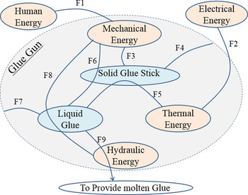
In the first approach, the modeling begins with defining the boundaries of the system or artifact to be designed, recognizing different elements of the systems’ environment in order to satisfy the final aim of the system. In the glue gun case, the final aim is to deliver a controlled amount of molten glue. The input material is in the form of solid glue and the output material is the molten glue. The system requires thermal energy to melt the glue. To start with similar initial conditions for both our both modeling approaches, it is assumed at first glance that the primary energy used to provide heat is electrical energy, and the mechanical energy to feed the glue stick is provided by human energy. The solid glue is used in two functions, to provide hydraulic energy to push the liquid glue out of the nozzle and also to change the state of the solid glue into liquid glue. The associated energy domains and materials in the glue gun are shown in different colors in Figure 19 (i.e., orange for energies and blue for materials). Afterward, the necessary functions are defined between different energies and materials. While some functions can only be defined between energies or between materials, some other functions need to use an energy domain to act between two materials. For example, as shown in Figure 19, the solid glue stick is transformed into a liquid glue stick (F5) by using thermal energy. The functions shown in Figure 19 are systematically defined in Table 6. Each function is also given an approximate sequence and sorted according to the order in which this function becomes active. The active functions in the same time interval in Table 6 are represented in parallel in Figure 20. The function schematic shows each function in the form of input and output. Having the input, output, and time sequence interval for each function helps us to know how the functions are connected. To relate two functions together, we need to match the output of the function to the input of the function in the next time sequence interval.

Fig. 19. Schematic view of associated functions in the glue gun.

Fig. 20. Glue gun function model based on function schematic interaction.
Table 6. Function definition for schematic view of the glue gun's associated functions

The function model based on this initial analysis is represented in Figure 20. It should be mentioned that the modeler has a significant impact on the nature of the model. For example, one might think that the pressure on the liquid glue stick can be provided by directly pushing the glue stick by hand or by an indirect action performed on the glue stick, or even by a specific device generating pressure on the liquid glue.
The second approach used to present the model of the functional architecture is a purely reverse engineering approach. In this approach, existing design architecture is available, and the role of the modeler is to represent the functional model using the existing system as a reference. Later in this section, the function model will be used in the DACM framework to take the function modeling a step forward toward increasing the usability of the function modeling. The sequence of the required steps in the DACM framework was explained in the Section 3 (see Fig. 10).
5.1. Step 1: System definition
The modeling begins with systems definition and the purpose of the modeling. In this case study, the system is the whole glue gun, including its components, and the purpose of the modeling is to present a model supporting the later physics-based reasoning.
5.2. Step 2: Function modeling
A black box model is considered; the solid glue stick is the input material, and the human energy and electrical energy are the energy inputs. The human and electrical energies are used to push and melt the glue. At the other side of the black box model of the glue gun, we have the melted glue. After the trigger has been pushed, the human force is converted to mechanical work belonging to the mechanical energy domain. The mechanical force activates a mechanism to guide the glue stick and to grip it. The glue stick is melted in a dedicated area of the glue gun, and a compressed spring provides the backward movement of the trigger, allowing a new push on the trigger. On the other side, the electrical energy is converted into thermal energy, and this thermal energy melts the glue stick. A part of this thermal energy is also dissipated in the environment. The modification of the state of the glue from solid to liquid leads the energy to change from mechanical energy to hydraulic energy. The initial function model is represented in Figure 21. In the preparation of the function model that follows, a limited set of vocabulary is used. This vocabulary was presented in Table 1 in the Section 3. Figure 21 depicts a model resulting from numerous iterations. The limited vocabulary is used to converge in terms of representation details. It should be noted that the function model shown in Figure 21 is slightly different from the function model shown in Figure 20. The model is different in its architecture, and in Figure 20, the system used to pull back the trigger is not present. This main difference is that Figure 20 was not trying to abstract from any specific solution. The architecture in Figure 21 is also more detailed. This is due to the forced usage of a limited set of function vocabulary pushing the modeler to detail more the model.

Fig. 21. Initial function model of the glue gun.
The model in Figure 21 is used as a reference, and the DACM framework is now developed further. The functional boxes in the function model are mapped to the bond graph elements (Fig. 22). This is done by performing a one-to-one mapping between the functional representation shown in Figure 21 and the bond graph elements presented in Table 1. Knowing the primary function name provides a limited set of choices between bond graph elements. For instance, “connect” offers two possible bond graph elements: “flow junction” and “effort junction.” There is a clear difference between these junctions. A flow junction is used when we have flows of equal values between different “pipes” connecting at junctions. An effort junction is applied if the efforts arriving at an interface are equal. This kind of physics-based reasoning should be performed for each functional box to decide between the types of junctions to be integrated. These choices are fundamental to the validity of the final model. These choices are automated in the online platform developed to model the use of the DACM framework.
Table 1 and Table 7 represent the one-to-one mapping of the initial function model into a bond graph representation. Analyzing the initial bond graph reveals that the conversion of human force to mechanical force is performed by a “transformer” (TF4) element. The transformer converts translational force and velocity to torque and angular velocity, while we will need translational force and velocity after JE1. So the use of an additional transformer between the (TF4) and (JE1) elements is essential. Having this kind of critical physics-based reasoning in the bond graph can show if any required element is missed. Moreover, it will give an insight into the design solution even before attributing a physical artifact to the functions. It should be noted that the human force could be transferred to mechanical force with a single transformer if a direct human force is applied in the same direction as the movement of the glue stick. This is not the case in the architecture of the glue gun. This is consequently requiring a transformation of a linear movement into a rotational movement using a second transformer. This process requires satisfying the coherence of the model with the real glue gun architecture, and when this is obtained, it is possible to move to the next phase.
Table 7. Mapping from functional vocabulary to possible choice of bond graph elements

Now let us have a more detailed look at the thermal elements of the model (Fig. 22). The effort and flow variables are temperature and entropy flow rate, respectively. The multiplication of flow by effort shows the instantaneous power. Nevertheless, the entropy is not conservative and not directly measurable either. For those reasons, applying a true bond graph in the thermal domain is not straightforward. A pseudo bond graph, initially developed by Karnopp (Reference Karnopp1979), offers the possibility of using the heat flow rate instead of the entropy flow rate to characterize the flow. It provides more flexibility for presenting equations without losing the advantages of bond graph elements. Thus, another modification of the initial function model is to present the thermal aspect of the model in a pseudo bond graph. In a pseudo bond graph, the “heat flow rate” and “temperature” characterize the flow and effort, respectively. A pseudo bond graph can be systematically applied to a thermal process. With the hypothesis that the temperature is distributed nonhomogenously in the parts, each part is represented in a flow junction or with a divided flow function. The temperature remains constant at each contact surface. The interaction or the contact surface between parts or between parts and the surroundings is shown by the effort junction or with the connect function. In other words, we will have an effort junction between the flow junctions. The resistor and capacitor elements are connected via a flow junction and effort junction, respectively. The resistor element characterizes the heat transfer by conduction and convection.

Fig. 22. The initial bond graph model mapped from the initial function model of the glue gun.
Once again, the latest function model should be mapped to the bond graph elements using Table 7. In the next step, the variables are assigned to the bond graph representation.
5.3. Steps 3 and 4: Providing and assigning variables
Each energy flow between two functional boxes is mapped to variables in two categories: flow and effort. The flow and effort variables are selected on the basis of the energy domain in Table 1. In order to be able to distinguish easily between the different variables in the same category, a number is attributed to the repetitive variables. In addition to the flow and effort variables, some of the bond graph elements require the variables to be assigned inside the elements to generate the causality and define the characteristic of the element. As mentioned in the Section 3, the inside variables are categorized into the three categories of “displacement,” “momentum,” and “connecting.” The use of connecting variables is a major difference with the bond graph approach. This type of variable is allowing to really designing a system and not simply modeling the dynamic of a system. Table 8 represents the influencing variables of the model, together with their associated dimensions and categories.
Table 8. System variables with associated dimensions and categories

Figure 23 depicts the pseudo bond graph representation, mapped from the modified function model of the glue gun shown in Figure 24. The influencing variables are assigned to the pseudo bond graph representation. The transformer TF5 is added between TF4 and JE1 on the mechanical side of the model in comparison with the last bond graph representation. The transformer (TF4) transforms the translational force (F) and velocity (V) into torque (Tr) and angular velocity (w). From the other side of the model, the electrical energy and the difference in temperature between adjacent parts cause the heat flow. JE3 and JE2 represent the heating coil and glue stick. JF4 maps the heat exchange surface between “outer surface of coil and surroundings,” and JF3 shows the heat exchange surface between “the inner surface of the heating coil and the glue stick.” In addition, (e 5) shows the temperature difference between the outer surface of the coil (e 2) and the ambient temperature (e 4 = t a). The convection coefficient (H), heat surface exchange (A), and temperature difference (e 5) characterize the heat convection between the heat coil and the surroundings in the (R 1) element. In the same manner, the difference in temperature between the inner surface of the coil and the glue stick (e 6), conduction coefficient (K), and glue stick diameter (D) characterize the heat conduction between the heating coil and the glue stick in the (R 2) element.

Fig. 23. Pseudo bond graph representation filled with variables.

Fig. 24. Modified function model of the glue gun.
5.4. Steps 5, 6, and 7: Generating a colored causal graph and computing behavioral laws
Using the predefined causality rules for each bond graph element (see Fig. 11), a general causal graph and the governing equations are generated. This is a second major difference with the traditional bond graph approach. Colors are used, and the equations are derived using the DA theory (Coatanéa et al., Reference Coatanéa, Roca, Mokhtarian, Mokammel and Ikkala2016). Identifying incoming and outgoing variables will enable us to form the causal graph. An additional rule is that the exogenous variables are always the cause of outgoing variables. The causal graph shows the relation between variables in terms of cause and effect in a visual manner, and the set of equations relate the variables in a mathematical manner.
Figure 25 represents the causal graph of the glue gun model. The governing equations extracted are the causal graph and are listed in Table 9. DA is used to present equations between variables in the form of the product (Coatanéa et al., Reference Coatanéa, Roca, Mokhtarian, Mokammel and Ikkala2016). The other equations, in the form of equalities and summation of variables, are extracted from the junctions.

Fig. 25. Causal graph of the glue gun.
Table 9. Governing equations extracted from causal graph and dimensional analysis

5.5. Step 8: Qualitative simulation, contradiction analysis, and incremental innovation
Once the causal graph and set of governing equations of a problem are ready, the contradiction analysis can be performed. The contradiction analysis starts with choosing the qualitative objective of the performance variables (i.e., red variables) of the system. In the case of the glue gun, finding a design solution that lets the user provide molten glue with less effort and less energy consumption is desirable. Less energy consumption is partly related to the insulation condition of the system. However, it is also related to the final temperature of the output molten glue. Therefore, minimizing the output temperature of the molten glue (i.e., minimizing “e 8”) to a few degrees above its melting point can be considered to be the first qualitative performance. If the user can have a higher material flow rate while pressing the trigger, this satisfies the desired need to have molten glue with less human effort. Increasing the output material flow rate (i.e., maximizing MFR) is considered to be the second qualitative performance in this study. It should be mentioned that different qualitative performances can be considered that are based on different aims. The backward propagation as the result of considering the two above-mentioned performances is shown in the causal graph in Figure 26.

Fig. 26. Contradiction analysis in the causal graph.
Let us analyze the result of backward propagation shown in Figure 26. Maximizing the flow rate of molten glue (MFR) requires the volume flow rate (Q) to be maximized. Volume flow rate depends on multiple variables such as pressure (P), viscosity (μ), and the volume of molten glue [cross section (S) and length (L)]. Maximizing the flow rate requires maximizing or minimizing one or several of these variables. To increase the volume of molten glue (Q), we need to increase the pressure on the glue stick (P), and/or the cross section of the glue stick (S). Increasing the pressure has a direct relation with applied force, and a reverse direction with the glue stick cross section. Therefore, the first contradiction is detected, as we need to minimize and maximize the cross section (S) simultaneously (see Fig. 26). In contrast, based on the casual graph, to minimize the viscosity (μ), the temperature of molten glue (e 8) should be increased. The latter is in contradiction with the second objective of the study, which is to decrease the temperature (e 8). The backward propagation of the second objective (minimizing e 8) also indicates that the glue stick diameter (D) should be minimized to melt the glue stick faster and reduce the energy consumption. Figure 26 illustrates the backward propagation of the two qualitative objectives on the causal graph. The contradictions are highlighted on the causal graph. The result of the contradiction analysis and the visual causal relation between variables will guide where the designer should search for an idea to innovate or to improve the performance of the system. In addition to the principles of TRIZ (Altshuller, Reference Altshuller1999), the inventive principles based on the causal graph are presented in Figure 27. To suppress the contradiction and to present an innovative solution in the current case study, we used Principle 9. Principle 9 exists among the TRIZ principles and basically suggests dividing the object into other objects. Therefore, using several glue sticks with a small diameter can solve the contradictions in this case study. The pressure is applied to an area, which is equal to the sum of the cross sections of the glue sticks. Smaller diameter of glue sticks enables the faster melting and the sum of the cross sections can be increased without interfering with the fast melting condition. As a result of providing a new solution for suppressing the contradiction, the causal graph should be updated to see if the proposed solution causes another contradiction in the system or not.

Fig. 27. Some inventive principles for the causal graph.
6. CONCLUSION
The paper presented an approach developed in order to tackle some of the issues limiting the usage of functional modeling in the engineering design world. The key objective of this article was to demonstrate that an extension of the capability domain of function modeling can be developed to build physics-based reasoning models. The DACM framework presented in this paper is a concrete method to implement the theoretical FBS models presented in the literature. Other characteristics associated with function modeling, such as the variability of the models produced by different modelers, have been analyzed in this paper. In this article, since the DACM framework predominantly starts from a reverse engineering situation, it is required that the function model that is generated matches the structure of the artifact being analyzed. The final model produced by DACM is heavily dependent on the quality of the functional model. Nevertheless, DACM is not limited to be used in incremental design innovations. For this reason, different mechanisms have been proposed to refine the functional model progressively and to insure convergence in the direction of a single functional model. The DACM approach cannot yet guarantee that different modelers will obtain a similar functional model at the end of the DACM process. A study of case studies involving several modelers is required as a continuation of the research to develop further the DACM approach. The authors of the article are also developing an online platform for DACM in which an ontology combined with AI-based tools has been developed to support the initial function modeling process.
The case study has exemplified the usage of DACM in the context of the glue gun example. The design objectives retained by the authors for the glue gun were to diminish the energy consumption and the manual effort on the trigger to be employed by the user of the glue gun. Other design objectives can be considered, such as, for example, increasing the output flow rate of the glue gun or adjusting the temperature of the glue precisely. We encourage readers to apply the approach in other case studies and to contact us if support is needed to use the approach. The DACM transformation and reasoning process of the initial function model are based on solid scientific grounds, as all the elements that combine to form DACM are validated approaches. The novel aspect of DACM has been integrated into a more global approach. The method has already been tested and validated in multiple case studies, and the method is currently being used in different design and manufacturing domains. The authors of the article are eager to test the approach in other fields as well.
Hossein Mokhtarian is a joint doctoral student at Tampere University of Technology and Grenoble Alpes University. His research area is the modeling and simulation of additive manufacturing.
Eric Coatanéa is a Professor at Tampere University of Technology. He holds a doctorate from Aalto University in Finland and the University of West Brittany in France. Eric's research interests are system engineering, design methodologies, and manufacturing. Dr. Coatanéa is a member of the ASME society.
Henri Paris is a Professor at Grenoble Alpes University in France. His research interests are manufacturing and design methodologies. Dr. Paris is a member of the GSCOP laboratory and a member of CIRP.