


1 Introduction
Collisions at sea are a leading cause of ship casualties. Analysis by the European Maritime Safety Agency (EMSA) shows that 26% of accidents are collisions, with between 500 and 700 incidents per year recorded between 2011 and 2018 and representing a leading cause of fatalities (EMSA, 2019). Furthermore, between 2009 and 2018, 46 vessels greater than 100GT were lost as a result of collisions (Allianz, 2019). These events can, therefore, result in significant loss of life, damage and pollution to the marine environment.
In an effort to reduce these hazards, many researchers have proposed models to predict and quantify the likelihood of collisions. First, statistical analysis of accident data and aggregated vessel traffic data to derive incident rates (Bye and Almklov, Reference Bye and Almklov2019). Secondly, the use of expert judgement in the form of Bayesian networks or event trees (Hanninen, Reference Hanninen2014). Thirdly, the development of models to represent navigation safety through geometric route models (Pedersen, Reference Pedersen1995; Mazaheri and Ylitalo, Reference Mazaheri and Ylitalo2010; Li et al., Reference Li, Meng and Qu2012).
Maritime risk modelling is challenged to some degree by the relative infrequency at which collisions occur relative to the volume of traffic within an area. For example, in the South–West Lane of the Dover Straits, which is one of the busiest waterways in the world, of approximately 38,000 annual transits, there were an average of 1⋅2 collision per year between 2009 and 2013 (MAIB, 2014), a rate of 1⋅05 × 10−5 per transit. With a sample size of six collisions over a five-year period, the validity of predictions using statistical models is limited. By extension, in other waterways, where fewer vessels transit, and there are fewer collisions, these problems are exacerbated.
To overcome this, many authors have proposed the use of non-critical accident situations, near misses or encounters as a proxy measure for collision risk (Du et al., Reference Du, Goerlandt and Kujala2020). Within this body of work, the underlying premise is that for a collision to occur, two vessels must meet, and by determining where two vessels meet more often, the likelihood of a collision increases. This concept of meeting vessels has been interpreted as a ship domain, the surrounding effective waters which a navigator wishes to keep clear of other ships or fixed objects (Goodwin, Reference Goodwin1975). Where the domain of a vessel is breached, a threat to navigational safety has occurred (Pietrzykowski and Uriasz, Reference Pietrzykowski and Uriasz2009). Such a model has good utility for application in collision avoidance and waterway risk management (Szlapczynski and Szlapczynska, Reference Szlapczynski and Szlapczynska2017). When a vessel is moving faster or is less manoeuvrable, a larger domain may be desired.
Methods of determining the size and shape of the ship domain has been a topic considered by many authors, and within the academic literature a plethora of domain shapes and sizes have been proposed (Pietrzykowski and Uriasz, Reference Pietrzykowski and Uriasz2009; Wang et al., Reference Wang, Meng, Xu and Wang2009; Szlapczynski and Szlapczynska, Reference Szlapczynski and Szlapczynska2017; Bakdi et al., Reference Bakdi, Glad, Vanem and Engelhardtsen2019; Fiskin et al., Reference Fiskin, Nasiboglu and Yardimci2020). Whilst we do not wish to repeat the extensive reviews of ship domains contained in other studies (see for example Fiskin et al., Reference Fiskin, Nasiboglu and Yardimci2020), we highlight some of the key ship domains in the following. An elliptical domain (Fujii and Tanaka, Reference Fujii and Tanaka1971) is shown in Figure 1(1); a segmented domain is shown in Figure 1(2) (Goodwin, Reference Goodwin1975); and Figure 1(3) shows a more complex domain with four axis, which lengths may vary depending on certain conditions (Wang, Reference Wang2010).

Figure 1. Selected ship domain concepts
Authors have generally acknowledged that the size and shape of the ship domain can change depending on several factors, including the physical characteristics of the vessels, the COLREGS situation, manoeuvrability, the human element, metocean conditions and fairway characteristics, amongst many others (Tu et al., Reference Tu, Zhang, Rachmawati, Rajabally and Huang2017). Each model is fitted to the local conditions and research question of the particular study, and it should not be expected that domains in constrained waterways would be similar to those in open waters (Wang and Chin, Reference Wang and Chin2016). The diversity of proposed domains is in some ways reflective of the lack of agreement on their structure and, therefore, would impact their predictive capability at determining collision risk (Goerlandt and Kujala, Reference Goerlandt and Kujala2014).
Szlapczynski and Szlapczynska (Reference Szlapczynski and Szlapczynska2017) and Fiskin et al. (Reference Fiskin, Nasiboglu and Yardimci2020) both draw a distinction between the methods through which domain models may be developed, such as analytically or empirically. We may also add ship domains that are developed using real-world trials, such as through the work of Yim et al. (Reference Yim, Kim and Park2018). Empirically derived ship domains have some attractions, able to represent how vessels actually behave, arguably reducing the risk of biases during domain definition and increasing validity as opposed to other methods. In addition, provided enough encounters are analysed, different influencing factors can be taken into account (Tu et al., Reference Tu, Zhang, Rachmawati, Rajabally and Huang2017). However, as is described in the following section, there are significant challenges with this approach, which mean that only a few studies have attempted to derive a ship's domain empirically (Szlapczynski and Szlapczynska, Reference Szlapczynski and Szlapczynska2017; Fiskin et al., Reference Fiskin, Nasiboglu and Yardimci2020), and the authors are aware of none that take into account multiple spatial and environmental factors.
Within this paper we propose and implement a method by which the critical passing distances between vessels can be mined, and the factors that influence those passing distances determined. We demonstrate that through the implementation of a machine learning algorithm to predict the domain size, based on the conditions of millions of historical interactions between vessels, many of the aforementioned limitations can be addressed. As a result, our work allows a flexible and intelligent ship domain which is evidence based. We then apply this domain to analyse collision risk across a large region. This paper is structured as follows: the remainder of Section 1 describes the key literature for empirical domain analysis and collision risk. Section 2 describes the datasets, methodology and model implemented within this project. Section 3 describes the results of the analysis and accompanying discussion, and conclusions are contained in Section 4.
1.1 Developing empirical domains
As defined by Fiskin et al. (Reference Fiskin, Nasiboglu and Yardimci2020), one of the methods to define the size and shape of a domain is empirical, using historical data of previous encounters. Perhaps the earliest example of this is Fujii and Tanaka's (Reference Fujii and Tanaka1971) work, which used photographs of radar screens in Japanese waters to establish the separation between vessels, identifying an ellipse of approximately 500 m by 300 m. This ellipse varied depending on ship length, but other factors were noted as likely having an influence. Similarly, Goodwin's (Reference Goodwin1975) analysis of the Dover Straits conceptualises domains in terms of three circular segments with fixed radius of 0⋅85 nm, 0⋅7 nm and 0⋅45 nm, rather than smooth elliptical shapes. Such a significant difference is reflective of the local nature of each survey, with different navigational dispositions (Fiskin et al., Reference Fiskin, Nasiboglu and Yardimci2020).
With the advent of the vessel tracking system AIS (Automatic Identification System), other authors have employed more extensive data-mining algorithms to determine domain size and shape. The workflow typically consists of processing AIS data, conducting a pairwise comparison of vessel positions, plotting these encounters and then deriving some form of a ship domain based on the results. Within previous studies, a number of different factors have been identified as likely influencing a domain's size or shape (Tu et al., Reference Tu, Zhang, Rachmawati, Rajabally and Huang2017; Fiskin et al., Reference Fiskin, Nasiboglu and Yardimci2020), yet analysis is generally limited to only three, namely vessel size, vessel speed and waterway type.
The EfficenSea (2012) project in the Baltic Sea tested and supported Fujii and Tanaka's (Reference Fujii and Tanaka1971) work in several locations by producing heatmaps of passing distances. Whilst they observed from the heatmaps that the distributions are influenced by vessel size, speed and study area, with for example restricted channels having closer passing distances than more open waterways, these effects are not quantified. Gucma and Marcjan (Reference Gucma and Marcjan2012) also used AIS to analyse the distributions of passing distances between different types of vessels and encounter situations. Their results suggest an asymmetric shape and that vessel type had little impact. Like many studies, their analysis focuses on an area of the Baltic Sea, specifically excluding ports, which might have different encounter characteristics.
Hansen et al. (Reference Hansen, Jensen, Lehn-Schiøler, Melchild, Rasmussen and Ennemark2013) analysed encounters at three locations in Danish waters, thereby providing some differentiation of spatial factors in encounters. They concluded that vessel domains are best described as ellipse shapes, similar to the results obtained by Fujii and Tanaka (Reference Fujii and Tanaka1971). The dimensions of their ellipse are eight ship lengths by 3⋅2 ship lengths but were derived visually on the resulting heatmaps, that were approximately on the 7⋅5% threshold. Pietrzykowski and Magaj (Reference Pietrzykowski and Magaj2016, Reference Pietrzykowski and Magaj2017) compared domains within a traffic separation scheme (TSS) precautionary area, again defining an elliptical domain through determining the distances of the 7⋅5th percentile of encounters. Their work also notes that vessels on average transit closer together within precautionary areas as they would within traffic lanes.
The aforementioned models have used relatively simple techniques to derive domain shapes. A more analytical approach is proposed by Wang and Chin (Reference Wang and Chin2016), who conducted domain modelling within the Singapore Straits, analysing more than 250,000 vessel interactions. They employed a genetic algorithm, utilising a weighting of distance, to determine the angular, size and speed coefficients of domains under different circumstances, quantifying for example the significant influence of vessel speed on domain size. Zhang and Meng (Reference Zhang and Meng2019) also study the Singapore Straits, developing a novel probabilistic ship domain, concluding that vessel speed and waterway characteristics had a significant influence on domain size.
A recent study measured ship domains by mining the characteristics of more than 600,000 encounters at 36 specific locations around the Swedish coast (Horteborn et al., Reference Horteborn, Ringsberg, Svanberg and Holm2019). They also find that the type of waterway, whether restricted or open sea, influences the domain size, as vessels must necessarily navigate closer together. Other outcomes suggested that the type of encounter influences the domain shape, but that vessel type and size had little influence.
The use of empirically calibrated vessel domains has several advantages. They enable an evidence-based assessment of vessel interactions, without relying on subjective inputs or defining a priori what collision situations are. Yet, determining empirical models of ship domains have three key challenges. Firstly, proposed methodologies are unable to capture or separate the impact of multiple, interrelating variables and, therefore, previous studies typically utilise only a few factors (Wang and Chin, Reference Wang and Chin2016). Secondly, such studies are isolated to single case studies of specific waterways (Szlapczynski and Szlapczynska, Reference Szlapczynski and Szlapczynska2017; Zhang and Meng, Reference Zhang and Meng2019) and, therefore, lack generalisation to other study areas, such as between ports and the open sea. Thirdly, the vast volumes of data required to be reflective of different conditions and waterway characteristics makes this approach computationally expensive. Furthermore, others have proposed that additional factors should be included, such as weather, daylight and fairway conditions (Horteborn et al., Reference Horteborn, Ringsberg, Svanberg and Holm2019). Within this paper, we seek to address these research gaps.
2 Data and methods
2.1 Vessel traffic data
The Marine Cadastre (2020), a joint project by the Bureau of Ocean Management and the National Oceanic Atmospheric Administration, publish AIS data collected from the US Coast Guard's national network of AIS receivers. Two seasonal samples were extracted for all regions between 1 January 2018 and 31 January 2018, and 1 June 2018 and 30 June 2018. The data is approximately one-minute resolution containing dynamic positional data, such as latitude, longitude, timestamp (UTC), course and speed and vessel identification attributes, such as MMSI number, vessel type and vessel size. The data covers a variety of different environments and waterway configurations, with offshore, coastal and inshore waters all represented.
It should be noted that the Marine Cadastre data does not provide AIS offsets, and only the vessel GPS position. As such, it is not possible to perform a correction to find the centroid of the vessel and, therefore, the domains may be off centre, introducing an error in the vessel position in the subsequent calculations. Given the size of vessels in the study, this error would rarely be greater than 100 m.
The data was extracted and processed following a number of steps. Firstly, we undertook linear interpolation of the vessels position, speed and direction in order to standardise the data at set one-minute intervals to allow for direct comparison. Secondly, where a vessel's heading is unavailable, we utilised the vessel's course to calculate interaction angles. Thirdly, any missing attributes in the data were filled in using the median values.
It should be noted that a one-minute resolution interpolation is coarser than that used in previous studies, such as one-second (Horteborn et al., Reference Horteborn, Ringsberg, Svanberg and Holm2019), ten-seconds (Rawson et al., Reference Rawson, Rogers, Foster and Phillips2014) or 30-seconds (Hansen et al., Reference Hansen, Jensen, Lehn-Schiøler, Melchild, Rasmussen and Ennemark2013; Zhang and Meng, Reference Zhang and Meng2019). However, we compensate for this through volume, which allows us to analyse many encounters under a greater variety of conditions, with 77 million and 125 million vessel positions in January and June 2018, respectively.
2.2 Approach
Three key methodological issues need to be addressed; firstly, how can we efficiently derive a dataset of encounters and associated temporal or spatial factors? Secondly, how should an encounter between two vessels be judged as a significant encounter? Thirdly, how can a machine learning model be used to predict the significant encounter distance in any situation? The methodological approach undertaken to achieve this is shown in Figure 2 and described next.

Figure 2. Domain workflow framework
Firstly, a pairwise comparison of all vessel positions within 3 km of each other is conducted. The choice of this distance is critical; greater distances will include more encounters, increasing both processing and the average passing distance between vessels. Previous studies have used varying distance thresholds, in both Wang and Chin (Reference Wang and Chin2016) and Pietrzykowski and Magaj (Reference Pietrzykowski and Magaj2016, Reference Pietrzykowski and Magaj2017), a 2 nm (3⋅7 km) search radius is chosen without justification, whilst in Horteborn et al. (Reference Horteborn, Ringsberg, Svanberg and Holm2019) a 5 km distance is utilised. Hansen et al. (Reference Hansen, Jensen, Lehn-Schiøler, Melchild, Rasmussen and Ennemark2013) use a 3⋅5 km distance, justified as 10 times the longest ship in the dataset. Arguably the distance should be greater, such as at 6 nm, the usual observation range of ship-borne radar in coastal areas (Zhang et al., Reference Zhang, Goerlandt, Kujala and Wang2016).
Secondly, we determine that 1 in 10 encounters would be critical for determining domain distance, such that 90% of encounters are considered safe. To determine this, we need to identify the closest 20% of encounters for each combination of circumstances (vessel type, location, speed and others), and develop a regression model to create a best fit that is approximate to the 10% threshold. Other thresholds have been suggested by other authors, such as 5% (Horteborn et al., Reference Horteborn, Ringsberg, Svanberg and Holm2019) or 7⋅5% (Hansen et al., Reference Hansen, Jensen, Lehn-Schiøler, Melchild, Rasmussen and Ennemark2013; Pietrzykowski and Magaj, Reference Pietrzykowski and Magaj2016).
The determination of both the critical search distance and percentage threshold for domain size are arbitrary to an extent, and the results of the analysis are sensitive to the chosen values. For example, Horteborn et al. (Reference Horteborn, Ringsberg, Svanberg and Holm2019) use 5 km and a 5% threshold, whereas we use a 3 km and 10% threshold, which would be similar, but we require significantly less computations between ship pairs. We have sought to utilise logical and practicable thresholds but invite further work to assess the sensitivity of the results to other thresholds.
The workflow to identify encounters is similar to those proposed by previous authors in the literature review. Firstly, the AIS data is interpreted to one-minute resolution using a linear method to standardise the AIS dataset temporally. Secondly, a pairwise comparison at every timestamp was conducted, with only those records retained where the haversine distance between the vessels was less than 3 km and the average speed of the vessels greater than 1 kt. The retained results are spatially indexed to enable joining with metocean and other spatial datasets.
During data exploration, it was determined that some encounters occur frequently and are the result of normal operational behaviours. For example, in ports, tugs and pilot boats will come alongside navigating commercial vessels, yachts might be racing in groups, or fishing boats may operate in pairs. Each of these situations would generate encounters, and whilst a collision might still occur, they do not reflect the normal navigational practice between vessels. To account for this, we limit the encounters to the following pairs which are unlikely to exhibit such issues:
1. Commercial ship versus commercial ship
2. Fishing versus Recreational / Recreational versus Fishing
3. Commercial versus Fishing or Recreational / Fishing or Recreational versus Commercial
Thirdly, a machine learning algorithm is utilised to predict the critical passing distance between vessels under different conditions through regression. To achieve this, the 20% closest values for each encounter circumstance are extracted, split into a training and testing dataset for evaluation, before random forest regression is utilised to predict the passing distance for all of the input conditions.
2.3 Feature selection
For each of the 5 million resulting encounter pairs, a set of features are identified and used to categorise the type of encounter. Table 1 shows the features used in this assessment and these will be discussed in turn. In order to identify the closest 20% encounters of each configuration, it is necessary to reduce some of these continuous features into categorical scales to support computation. Increasing the number of categories for each feature would increase the resolution of the analysis but reduce the sample size within each category. It should be noted that the choice of these categories would have some influence on the results, and, therefore, the rationale has been provided where this has been undertaken.
Table 1. Model features

2.3.1 Bearing
For each encounter, the relative bearing (α) from vessel 1 to vessel 2 can be calculated as the difference between the heading of vessel 1 and the geographic bearing with vessel 2 (see Figure 3). In Horteborn et al. (Reference Horteborn, Ringsberg, Svanberg and Holm2019), 5° bearings are used, whilst Fiskin et al. (Reference Fiskin, Nasiboglu and Yardimci2020) use both eight and 16 nodes. In our case, we also use eight nodes at 45-degree groupings, such that each value is ±22⋅5°, i.e. 090° includes 067⋅5° to 112⋅5° (see Figure 3).

Figure 3. Calculation of vessel positions/encounter situations (left) and domain sectors (right)
2.3.2 Encounter type
The heading differential between the two vessels can be calculated and used to define the encounter situation in line with the International Collision Regulations. The categories are as follows (Montewka et al., Reference Montewka, Hinz, Kujala and Matusiak2010):
• Head On – 170–190 degrees
• Overtaking – 350 to 10 degrees
• Crossing Stand On – 190 to 350 degrees
• Crossing Give Way – 10 to 170 degrees
2.3.3 Distance from shore
Distance from shore was calculated using a high-resolution vector world landmass shapefile, converted into a 500 m resolution raster and the ESRI ArcGIS Euclidian Distance function performed to calculate the distance from each raster cell to the closest cell containing shoreline. This has been categorised between coastal and offshore waters using the 12 nm limit, and 5 km used to differentiate port and inshore waterways.
2.3.4 Vessel speed (SOG)
Provided by AIS data, categorised into five knot bands up to 15 knots.
2.3.5 Vessel size
Provided by AIS data, categorised into three groups of less than 50 metres (including the majority of fishing and recreational craft) and greater or less than 250 m. This separates commercial vessels into two size groups based on the approximate size of an Aframax or Panamax vessel. This enables a comparison between the domain characteristics of the largest commercial vessels from the majority which are less than 250 m.
2.3.6 Vessel type
Provided by AIS data, categorised into commercial cargo or tanker vessels, fishing vessels and recreational craft, as described in Section 2.2.
2.3.7 Near TSS
Some in the literature have proposed that ship routeing measures effect encounter characteristics. To test this, an additional feature was included which determined whether the encounter occurred within 2 nm of a TSS, including traffic lanes and precautionary areas. Spatial data files of these features are provided by the MarineCadastre (2020).
2.3.8 Near port
Whether the encounter was within 20 nm of a major US port – this includes approach channels and port limits. These details are available from The National Transportation Atlas Database (USDOT, 2020). A more accurate delineation could be achieved by marking the waterways of each individual port; however, at a national scale this is not practical.
2.3.9 Wind speed
Wind speed at time of encounter was derived from the EU Copernicus Earth Monitoring Service. A NetCDF file containing time, location and wind speeds was extracted for June 2018 from dataset WIND_GLO_WIND-L4_NRT_OBSERVATIONS_012_004. This dataset contains wind speeds at six hourly temporal resolution and 0⋅25-degree spatial resolution. For each grid cell, the data was interpolated to one hourly resolution and joined to the encounter dataset based on its time and location.
2.3.10 Day/Night
Based on the UTC, latitude and longitude of the encounter, a spatial query was conducted to determine the local time zone. Any record between 06:00 and 18:00 is categorised as a day encounter and between 18:00 and 06:00 categorised as a night encounter.
2.4 Random forest prediction of domain distance
From the 1 million encounters that account for the 20% closest encounters in each group, a regression problem can be framed to predict the passing distance given the characteristics of that encounter. Given the multiple factors which influence ship behaviour and risk perception, we propose that a machine learning algorithm can be utilised to learn the domain size and shape of a given vessel in a given situation. In this case, we utilise the random forest algorithm in the scikit-learn package of Python. Random forests (RF) (Breiman, Reference Breiman2001) are a popular ensemble-tree learning algorithm which have been applied to many regression and classification problems in maritime contexts (Jin et al., Reference Jin, Shi, Yuen, Xiao and Li2019). Whilst many other regression algorithms are available, we utilise RF due to its widespread popularity and availability in numerous languages as well as inherent properties, such as training speed and robustness when using high-dimensional and unbalanced datasets (Breiman, Reference Breiman2001).
RFs consist of many (k) decision trees, which themselves consist of a root node, child nodes and terminal nodes. The root node consists of training data, which is split into a child node based on attribute variables and maybe further split into subsequent child nodes. The algorithm seeks to ensure that each child node is as homogenous as possible, and when this is reached the node becomes a terminal node. Decision trees are prone to overfitting, as they are capable of replicating the structure of the training data perfectly. To overcome this, RFs introduce bagging and random subspace into the algorithm. Bagging (bootstrap aggregating) involves the training dataset being sampled with replacement, and random subspace involves randomly selecting attribute variables when splitting the dataset. Figure 4 shows a schematic of RF, with the training dataset sampled and then decision trees constructed, with the average of the predictions of each tree used as the resultant prediction. As a result, RFs are an ensemble of decision trees, avoiding overfitting by producing a diversity of trees.

Figure 4. Schematic of random forest regression
In addition, RF allows for the calculation of the relative importance of each feature in producing the predictions. Feature importance, also referred to as Gini importance, is calculated by comparing how much the tree nodes that use each feature reduce the impurity on average (Breiman et al., Reference Breiman, Freidman, Stone and Olshen1984).
The data is split into a training and testing dataset, with an 80:20 ratio, and a RF trained on the training dataset only. Hyperparameter tuning was performed using a random search of a hyperparameter grid using cross-validation, with the best performing parameters selected based on the ‘r2’ scoring, which achieved 0⋅74 on the training set. The selected regressor was then applied to predict the passing distance on the test set, with an r 2 of 0⋅69. It should be noted that by segmenting the dataset in Section 3.3 into the top 20% of each category, we ensure that the dataset is not imbalanced by the encounter types that are most common and therefore avoid overfitting
3 Results and discussion
3.1 Mined encounter densities
In order to establish how encounters change in given conditions, we first plot the densities of interactions between commercial vessels in Table 2. Within these plots, one ship is located at x = 0/y = 0, heading due north, and the densities show the most frequent positions where encounters are recorded. Therefore, to interpret this plot, if an area of high density is seen at for example, x = −1000 and y = 0, this means that a greater propensity of encounters occur for a transiting vessel, on the port (left) side as it transits.
Table 2. Commercial encounter density – speed greater than 5 kts

Vessel is orientated north-up at x = 0, y = 0. Distances in metres.
The densities demonstrate that the distribution of encounters changes significantly with encounter type and distance from shore, supporting previous work (Horteborn et al., Reference Horteborn, Ringsberg, Svanberg and Holm2019). For example, in constrained waterways, vessels must necessarily pass each other with less separation than they might otherwise choose offshore.
For head-on encounters, it can be seen that the highest density of encounters occurs on the port side. This reflects Rule 14 of the collision regulations that requires two vessels meeting on reciprocal courses to both turn to starboard to pass each other on the port side. This results in an asymmetric domain that has been previously highlighted (Goodwin, Reference Goodwin1975).
Overtaking encounters are described under Rule 13 of the collision regulations, such that the overtaking vessel avoids the other vessel. Within our data, in the coastal locations, a clear ring can be seen as vessels overtake one another, leaving sufficient sea room to keep clear. For both the inshore and to some extent the coastal regions, the high density approximately 2 km ahead and astern indicates the natural separation. At the centre of the overtaking offshore plots, two areas of high-density are vessels moored alongside one another conducted ship-to-ship transfers (STS), are removed from the subsequent modelling as they are outliers for our purposes.
Crossing situations have been compared for stand-on and give-way situations as defined under Rule 15 of the collision regulations. These state that when two vessels cross one another, the vessel on her own starboard (right) side shall keep clear of the other, avoiding crossing ahead. Therefore, in the context of our stand-on plots, the other vessel is necessarily crossing left to right, and for the give-way plots, the other vessel is crossing right to left. Taking the coastal region as an example, the data shows that a give-way vessel would cross a stand-on vessel's course approximately 2 km ahead, or alternatively would cross astern at a similar distance, a pattern similar to that shown in Hansen et al. (Reference Hansen, Jensen, Lehn-Schiøler, Melchild, Rasmussen and Ennemark2013). Offshore, a greater proportion of vessels choose to cross astern rather than ahead of a stand-on vessel. Inshore, with linear channels, the crossing potential for commercial ships is limited, and therefore a similar but less well-defined pattern is evident.
3.2 Influence of factors on domain size and shape
Understanding the reasons why passing distances and domain shapes vary has been a focus of several previous studies (Horteborn et al., Reference Horteborn, Ringsberg, Svanberg and Holm2019). Figure 5 shows a correlation matrix of each of the features investigated in this study, in order to determine whether there is correlation between the different independent features. Weak positive correlations indicate that vessel speed, length, weather and traffic schemes have a minor impact on domain size, whilst the passing distance is inversely correlated with the presence of ports. Individually these correlations are weak and without statistical significance, which has been concluded by others (Horteborn et al., Reference Horteborn, Ringsberg, Svanberg and Holm2019). However, in Section 3.1 we have demonstrated that by combining factors, much clearer patterns emerge, which are demonstrable through our implementation of machine learning.

Figure 5. Correlation matrix for exploratory variables
Through application of RF, we can measure the feature significance towards the model predictions across our exploratory features, which is shown in Figure 6. In each case, we will examine the impact of these features on certain domain shapes.

Figure 6. Feature importance
The most significant feature is distance from shore, with vessels navigating naturally closer together when they are in confined waterways. This is demonstrated in Figure 7 for head-on and overtaking commercial encounters. The circumstances of an encounter in a narrow channel would likely be seen as typical in that situation, whereas were the same encounter distance to occur offshore, it might be seen as a near miss. It is also of note that there is a difference between the two encounter types shown in Figure 7, with overtaking encounters exhibiting a more elliptical shape (such as described by Fujii and Tanaka, Reference Fujii and Tanaka1971), with little difference between coastal and offshore waters, whereas head-on domains are offset to starboard, with a much greater size difference, perhaps due to a greater perceived risk of collision in head-on situations. These biases to starboard are evident in some of the segmented domains proposed, for example by Goodwin (Reference Goodwin1975).

Figure 7. Commercial ship head-on (left) and overtaking (right) encounters at different locations. Distances in km
The second most significant features are vessel speed and vessel length for the two vessels involved in the encounter. With respect to speed, it is logical that the faster a vessel is travelling, the greater the safety distance the master wishes to keep as the opportunity to either stop or manoeuvre clear reduces. Figure 8 shows commercial ship overtaking encounters at various speeds, demonstrating a clear increase in the natural domain size as the vessel increases. This effect is approximately a doubling between less than 5 kts and 10–15 kts, an effect which has been observed by others (Wang and Chin, Reference Wang and Chin2016; Zhang and Meng, Reference Zhang and Meng2019). Figure 8 can be directly compared to Wang and Chin (Reference Wang and Chin2016) showing a similar overtaking forward distance of between 1 km and 1⋅5 km for a commercial ship travelling 15–20 kts. However, our domains are less elliptical in nature, possibly due to the greater range of locations under assessment.

Figure 8. Left – commercial ship overtaking encounters at various speeds, right – all overtaking encounters by vessel size. Distances in km
Vessel size was also shown to influence domain size and shape with larger vessels generally maintaining a greater separation from other vessels (see Figure 8). Previous work has shown that this effect is limited (Horteborn et al., Reference Horteborn, Ringsberg, Svanberg and Holm2019); however as previous work has typically considered only commercial shipping, it is likely that our inclusion of recreational and fishing vessels would increase this effect.
The third group of factors include wind speed, proximity to ports and traffic schemes are shown to be less significant than the aforementioned variables. In significant weather conditions, vessels are affected by windage and other phenomenon that impact the safe handling of a vessel, and as such, it would be sensible to increase the passing distance between one another. Figure 9 shows overtaking commercial vessel encounters in coastal and offshore waters and suggests that this effect is only significant once wind speeds exceed 10 m/s (Beaufort Force 6), providing empirical evidence to support similar conclusions based on ship motion modelling (Szlapczynski et al., Reference Szlapczynski, Szlapczynska and Krata2018; Szlapczynski and Krata, Reference Szlapczynski and Krata2018). It should be noted that as the metocean data is averaged at six hourly intervals, isolated squalls and gusts are not captured within this analysis and may result in more significant variations than we are able to describe.

Figure 9. Commercial ship overtaking encounters by wind speed. Distances in km
Figure 10 compares the domain shapes on overtaking situations between commercial vessels within traffic schemes and near ports. It is surprising to see TSS as one of the least significant factors shown in Figures 5 and 6, this being one of the key risk control measures that can be put in place by regulators and governments. Traffic lanes seems to slightly reduce the domain width, perhaps indicating that the predictable linear flows in traffic schemes increase the comfort of the bridge team in overtaking at closer distances. With this said, on average the presence of a TSS has little impact, as the circumstances of the individual encounter are more significant. This might partly explain why more elliptical domains are derived when studies are performed in areas with a TSS, such as Wang and Chin (Reference Wang and Chin2016).
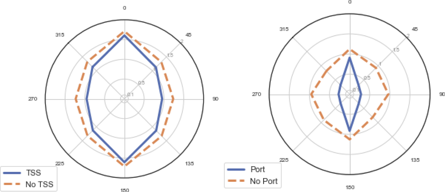
Figure 10. Commercial vessel overtaking encounters between traffic schemes and ports. Distances in km
Port approaches and waterways have a more significant influence at reducing the domain size due to the constricting effect of buoyed waterways that necessitates closer interactions, a similar effect as the one shown in Figure 7. The significance of this difference is such that some authors have chosen to either exclude these waters (Gucma and Marcjan, Reference Gucma and Marcjan2012) or concentrate on them entirely (Rawson et al., Reference Rawson, Rogers, Foster and Phillips2014).
Whilst it has been suggested that daylight might be a contributory factor (Horteborn et al., Reference Horteborn, Ringsberg, Svanberg and Holm2019), within our exploratory data analysis there was no clear evidence and, therefore, it has not been included within our modelling. The greatest effect of this factor is the temporal variation in the volume of fishing and recreational traffic throughout the day.
These results demonstrate that domain size and shape, and therefore the passing distances between vessels, varies based on numerous input conditions, including vessel size, speed, waterway conditions and weather. Therefore, attempting to utilise vessel domains that do not account for some of these conditions risks producing results that are skewed either in exaggerating or under-representing the frequency of interactions between vessels. For example, Figure 10 shows that the same ship domain shape or size cannot be applied both to ports and traffic lanes. By utilising machine learning, we have constructed a dynamic ship domain which can account for many more features than previous models and, therefore, better reflects the natural behaviour of vessels in meeting situations.
3.3 Application for collision risk assessment
Having trained and calibrated our empirically derived ship domain, we can then utilise it to study where critical encounters are more likely to occur. Many previous studies have utilised analysis of the frequency and spatial variation in domain encounters a measure of collision risk (Du et al., Reference Du, Goerlandt and Kujala2020). Within this section we seek to assess domain encounters between commercial vessels in the Puget Sound between Washington State and Vancouver Island. Figure 11 shows the density of commercial shipping in the region, clearly identifying the major routes as vessels enter the Strait of Juan de Fuca and the TSS, before proceeding north to Vancouver or south to Seattle.

Figure 11. Transit density in Puget Sound
Figure 12 compares the frequency of critical encounters as derived from our model. These are where two vessels encounter at a closer distance than the critical encounter distance predicted for those circumstances, as defined in the previous sections. The results show that certain regions have a far greater number of encounters than would be expected given the level of traffic. For example, the Haro Strait to the east of Victoria necessitates a constriction in the flow of traffic, increasing the number of encounters. The most significant areas of high encounters are near to ports and terminals, where both the density of traffic is greater, and the available sea room is less.

Figure 12. Critical encounters in Puget Sound
Whilst several studies have presented analysis of collision risk through the use of domain analysis (Goerlandt and Kujala, Reference Goerlandt and Kujala2014; Rawson et al., Reference Rawson, Rogers, Foster and Phillips2014), we argue that this approach has several advantages. Firstly, as our domain is empirically derived from previous transits, it reflects the natural behaviour of vessels in meeting situations, as opposed to other methods, such as expert judgement which might be subject to bias. Secondly, by utilising machine learning to construct the ship domain, we are able to integrate a far greater number of different features than other methods, allowing the algorithm to learn the domain shape in hundreds of different permutations of circumstances. This would not be possible utilising traditional methods. Thirdly, such an approach has good scalability; with more training data it would be possible to include other features, such as wave heights, visibility or extents pilotage districts, in order to further develop the model.
4 Conclusions
The results of the analysis presented in this paper support the wide body of literature concerning ship domains. Based on mining the passing distances between navigating vessels across a wide range of locations, environmental conditions and other circumstances, the size and shape of this domain can be derived. These domains clearly vary between locations, speeds and encounter types, supporting conclusions reached in previous work, but are influenced by other factors, such as weather, which have not previously been assessed. The analysis demonstrates that encounter distance is significantly less for inshore as opposed to offshore waters, low-speed to high-speed encounters and small vessels rather than large vessels. Whilst there is some evidence that higher wind speed and encounters outside of TSS lanes result in larger domains, this effect is less significant, and no evidence was found for the influence of day and night on domain size.
To capture all of these interrelating factors, we have developed a novel approach of utilising a machine learning regression algorithm to learn the passing distance between vessels in each circumstance. This ship domain is dynamic to ship speed, size, encounter type, weather and waterway characteristics, having trained on significant quantities of ship encounter data. To our knowledge, this is the first time that this proposed methodology has been applied to characterise ship domains. These learnt domains can then be applied to determine where critical encounters most frequently occur and inform maritime risk assessments.
Several other aspects of this research are open to further work. Firstly, we have discussed the apparently arbitrary method at which key parameters in empirical ship domain mining are derived, namely the maximum filtering distance and the ratio of critical to noncritical encounters. This gap is bridged when using nonempirical methods, such as expert judgement, but further work is needed to understand the sensitivity of empirical domains to parameter selection. Secondly, whilst we utilise a large amount of AIS data across a wide geographic area, we do not take advantage of any big-data processing technologies. The sheer volume of AIS data, and the computational complexity of calculating pairwise interactions between vessels can make scalability a challenge. Although some approaches have been proposed to streamline this process, such as reducing the raw AIS to simpler line segments (Horteborn et al., Reference Horteborn, Ringsberg, Svanberg and Holm2019), this limitation remains to some extent. Optimising domain calculations in big-data processing technologies such as Apache Spark would overcome this limitation by expanding the volume of data and variety of factors that could be investigated, but we are not aware of any previous research for this purpose.
The results show that it is possible to develop intelligent ship domain models, that better represent the usual navigation practice than traditional approaches. Through the use of a machine learning algorithm, a far greater number of influencing factors can be included in the subsequent domains than would be possible with traditional methods. Using models ill-suited to the local conditions under study can result in unrealistic results and therefore this has implications for the wider risk modelling literature.
Acknowledgements
This work is partly funded by the University of Southampton's Marine and Maritime Institute (SMMI) and the European Research Council under the European Union's Horizon 2020 research and innovation program (grant agreement number: 723526: SEDNA).


 Open access