


1. INTRODUCTION
TFRs (total fertility rate—the number of children expected to be born per woman) have been declining in both Europe and the US. This drop has been quite dramatic, falling from of around 3.0 children per woman in 1920 or 1930 to the current levels of 1.2–2.0 children per woman, depending on the country (with temporary increases of varying sizes, the ” baby booms”). While the downward trend is common to both sides of the Atlantic, the magnitude of the drop is not. For example, as of year 2000 the TFR was 1.2 in Italy, 1.3 in Germany, 1.8 in France, and 2.1 in the US (up from a minimum of about 1.8 in the 1980s). Thus, fertility is much higher in the US currently than in most of Europe. In 1920, in contrast, TFRs were higher than now both in the US and Europe but much closer to each other: 3.2 in the US, 3.3 in Denmark, 2.7 in France, 3.2 in Sweden, 4.1 in Spain, and so on. At that time, fertility in Europe and the US were roughly similar and they had been for nearly a century.
In summary, fertility rates in the US and the Western European countries were roughly similar early on in the 20th century; Between 1940 and 1955–60, depending upon individual countries, fertility increased in both the US and Europe, with the American’s increasing substantially more than the European average; this period is commonly known as the “baby boom.” After that, and for about forty five years now, TFRs have decreased but, again, the American one has decreased substantially less than the European generating a persistent difference in fertility rates between the two sides of the Atlantic.
This cursory review reveals two facts. First, that after the baby boom period, a new downward trend in fertility rates began in the late 1950s, which affected both the US and most of Europe. Second, that the downward trend was substantially stronger in Europe than in the US. This has led to a persistent difference of between 0.4 and 0.8 children between European and American TFRs. The first fact has a time dimension: fertility declined sharply over the 20th century, both in the US and Europe. The second is one of comparative statics: since the 1950’s fertility has been lower in Europe than in the US, and, moreover, the size of this difference has increased over time.
The timing of these changes, in conjunction with the idea that one of the principal motives for having children is for old age support, suggests the possibility that they might be related to the rapid expansion of government provided pension systems that took place over this period.Footnote 1 This coincidence in timing leads us to study the question more broadly. We construct a cross section of fertility and the size of government provided pensions (along with several other related variables) for 104 countries in 1997. We find a strong negative correlation, that is economically significant in size, between these two variables in the cross section.
Accordingly, in this paper we ask: What fraction of each of these three facts, the observed changes over time and differences in levels between US and European fertility and the cross-sectional observation from the 1997 data, can be accounted for by a single difference in policy—i.e., the timing and size differences in Social Security systems, both between Europe and the US, and across the world? The quantitative model we develop leads to the conclusion that about 50% of the time series drop, and about 60% of the comparative static difference, among and between the US and Europe can be accounted for by the (differential) growth of the national public pension systems. We also find that a large fraction (over 80%) of the differences in fertility identified in the cross section through regressions is also predicted by the same theoretical model.
The impact of changing fertility patterns and its connection to government provided pensions is not a new topic. Indeed, much of the literature on public pension systems points to the observed long term trends in fertility discussed above (along with ever growing life expectancies) as significant limitations on the financial viability of the current systems. What is less often discussed are the effects going in the opposite direction. That is, might the generosity of the pension plans themselves be one of the causes of these demographic trends?Footnote 2 This is the view that we explore in this paper.
In our analysis of cross-country data, we find that an increase in the size of the Social Security system on the order of 10% of GDP is associated with a reduction in TFR of between 0.7 and 1.6 children (depending on the controls included). These findings are highly statistically significant and fairly robust to the inclusion of other possible explanatory variables. Similar estimates are obtained when a panel data set of the US and a number of European countries is used. These results complement and improve upon earlier empirical work on both the statistical determinants of fertility and its relation to the existence and size of government run Social Security systems. Early work using cross-sectional evidence includes National Academy (1971), Friedlander and Silver (Reference Friedlander and Silver1967), and Hohm (Reference Hohm1975). Analysis of the relationship between Social Security and fertility based on individual country time series include Swidler (Reference Swidler1983) for the US, Cigno, and Rosati (Reference Rosati1996) for Germany, Italy, the UK and US, and Cigno, Casolaro, and Rosati (2002) for Germany.
Theoretically, we study the effects of changes of government provided old age pension plans on fertility in two distinct models—the Barro and Becker (Reference Barro and Becker1989) model of fertility (called the BB model subsequently) and the Caldwell model,Footnote 3 as developed in Boldrin and Jones (Reference Boldrin and Jones2002; labeled the BJ model subsequently). These two models are grounded in opposite assumptions about intergenerational altruism and, hence, intergenerational transfers. Both of them have a bearing on late age consumption and the means through which individuals account for its provision. In the BB model parents have children because they perceive their children’s lives as a continuation of their own. In the BJ framework parents procreate because the children care about their parents’ utility, and thus provide their parents with old age transfers. Thus, this is a formal implementation of what a number of researchers in demography would call the “old age security” motivation for childbearing. We find that in both models, any change in steady state fertility arising from changes in the size of pension systems works through general equilibrium effects, particularly through the effect on the steady state interest rate. Quantitatively, this effect is small in the BB model, but economically significant in the BJ framework. When the old age security motive dominates fertility choices, increases in the size of the public pension system decreases fertility, with perhaps as much as 50% of the reduction in fertility seen in developed countries in the past 50 years being accounted for by this source alone and over 80% of the difference seen in the cross-sectional study. Since government provided pensions are a larger portion of retirement savings for families at the low end of the income distribution our results are also consistent with the empirical finding that fertility has declined more for those individuals.
Within the Caldwell framework, we also consider the impact on fertility that results from improved access to financial instruments to save for retirement. Some of the empirical studies that have found evidence of a strong correlation between pensions and fertility have also reported a strong correlation between measures of accessibility to saving for retirement and fertility (e.g., Cigno and Rosati (Reference Cigno and Rosati1992).) We provide a simple parameterization of the degree of capital market accessibility and find that even relatively small reductions in financial market efficiency have strong impacts on fertility in the Caldwell model; societies where it is harder to save for retirement or where the return on capital is particularly low, ceteris paribus, have substantially higher fertility levels.
In sum, these findings give indirect support for a strong role for the “old age security” motive for fertility. As such, they are generally indicative of a more general hypothesis—Since children are perceived by parents as a component of their optimal retirement portfolio, any social or institutional change that affects the economic value of other components of the retirement portfolio will have a first order impact on fertility choices. The fact that models of children as investments work so well here, and in a fashion which is consistent, both qualitatively and quantitatively, with the data, is supportive of this basic hypothesis.
1.1. Relation with Earlier Work
The main contribution of this paper is to estimate the size of the effect of Social Security on fertility decisions by studying calibrated, quantitative, versions of the theoretical models. To our knowledge, no previous authors have undertaken such an endeavor, but a large literature exists that anticipates our work along various dimensions. Empirical analyses of the correlation between fertility indices and different measures of the size or the generosity of the public pension system go back to Hohm (Reference Hohm1975). He examines 67 countries, using data from the 1960–1965 periods and concludes that Social Security programs have a measurable negative effect on fertility of about the same magnitude as the more traditional long-run determinants of fertility, i.e., infant mortality, education, and per capita income.
Cigno and Rosati (Reference Cigno and Rosati1992) present a co-integration analysis of Italian fertility, saving, and Social Security taxes (SSTs). They study the potential impact on fertility of both the availability of public pensions and the increasing ease with which financial instruments can be used to provide for old age income. They conclude that “[...] both Social Security coverage and the development of financial markets, controlling for the other explanatory variables, affect fertility negatively.” (p. 333). Their long-run quantitative findings, covering the period 1930–1984 are particularly interesting in the light of one of the models we use here. The point estimates of the (negative) impact of Social Security and capital market accessibility on fertility are practically identical (Figure 8, p. 338) to what we find here.
The theoretical effects of pension systems on fertility have been studied extensively. Early work includes Bental (Reference Bental1989), Cigno (Reference Cigno1991), and Prinz (Reference Prinz1990) in addition to the original discussion in Becker and Barro (Reference Becker and Barro1988). More recent examples include Nishimura and Zhang (Reference Nishimura and Zhang1992), Cigno and Rosati (Reference Cigno and Rosati1992), Cigno (Reference Cigno1995), Rosati (Reference Rosati1996), Swidler (Reference Swidler1981, Reference Swidler1983), Wigger (Reference Wigger1999), Yakita (Reference Yakita2001), Yoon and Talmain (Reference Yoon and Talmain2001), Zhang (Reference Zhang, Zhang and Lee2001), and Zhang, Zhang and Lee (Reference Zhang, Zhang and Lee2001), among others. These papers cover different specifications of both models of fertility, as we do here, but are substantially more limited in scope and, in particular, they do not study the quantitative theoretical predictions of their models. For example, in both the Nishimura and Zhang and the Cigno papers, models are analyzed which are based on reverse altruism like that in Boldrin and Jones. However, they assume that all generations make choices simultaneously and hence, parental care provided by children does not react to changes in savings behavior. Moreover, they do not make the size of the intergenerational transfer endogenous, which, among other things, prevent them from considering the problem of shirking in parental care resulting from the public goods problem among siblings that is created when reverse altruism is present.
Closer in spirit to our work are the two articles by Ehrlich and Lui (Reference Ehrlich and Lui1991, Reference Ehrlich and Lui1998) in which the relation between exogenous SSTs, and endogenous fertility and human capital investment are analyzed using a model of intrafamily insurance markets. As in BJ, the motivation for having children comes from the old age security hypothesis, but the transfer from children to parents is assumed to be in fixed proportion to the investment, by parents, in the education of children. Their main result is that an increase in SSTs lowers fertility, savings, or human capital formation, and possibly all three, depending on parameter values and other details of the model. The theoretical message is, therefore, analogous to the one derived here. We add to their analysis by including capital accumulation, endogenizing the transfers from children to parents and conducting quantitative analyses of the effects. Ehrlich and Kim (Reference Ehrlich and Kim2005), is the paper that is closest to ours in terms of goals. Using an approach based on altruistic parents (i.e., similar to the BB model but also including both mate-search and human capital), they find that increases in the size of the Social Security system on fertility is negative, but smaller than what we find here. For example, in their baseline calibration, they find that decreasing SST rates from 10% to 0% increases fertility by approximately 0.1 children per woman. This effect is larger than what we find for the BB model, but this difference is probably due to the other differences in the models.Footnote 4
In studying the dynastic model of endogenous fertility we reach conclusions that are partially different from those advanced in the original papers. As mentioned above, Becker and Barro (Reference Becker and Barro1988) argue that a growing Social Security system should reduce fertility. Their analysis is based on a partial equilibrium argument according to which a Social Security system “...has the same substitution effect as an increase in the cost of raising a child [...] therefore [...] holding fixed the marginal utility of wealth [...], and the interest rate, we found that fertility declines in the initial generation while fertility in later generations does not change.” That is, there will be a transitional effect of lower fertility when the system is introduced, followed by a return to the original fertility level in steady state. Our analysis (see the Appendix for details) shows that, even in a partial equilibrium context, these conclusions are dependent on how fast the pension system grows, relative to the rate of interest. In a general equilibrium model, both the interest rate and the marginal utility of wealth adjust in such a way that an increase in fertility occurs in the new balanced growth path (BGP). Furthermore, there is no evidence in the data of a return to the previous level of fertility after a transition in those countries which have adopted a Social Security system during the last century, as would be predicted by the partial equilibrium argument.Footnote 5
A number of other authors in the demography and sociology literatures have provided evidence of the strong empirical link between parental dependence on offspring’s support in late age and fertility rates. This literature is too large to be fully reviewed here. Of particular note for our purposes are the papers by Rendall and Bahchieva (Reference Rendall and Bahchieva1998) and Ortuño-Ortín and Romeu (Reference Ortuño-Ortín and Romeu2003). Rendal and Bahchieva (Reference Rendall and Bahchieva1998) use data on poor and disabled elderly in the US to estimate the market value of the support they receive from relatives. These are largely in the form of time inputs in the household production function. They find that children are a valuable economic investment for the poorest 50% of the population even in the presence of current Social Security and old age welfare programs. Ortuño-Ortín and Romeu (Reference Ortuño-Ortín and Romeu2003) use micro data measuring parental health care effort and expenditure and also find substantial backing for the “old age support” hypothesis of fertility decisions.
In Section 2, we look at data: first we discuss the last 70 years or so of fertility both in Europe, and in the US, next, we present statistical evidence on the relationship between the size of the Social Security system and fertility using both cross section and panel data. In Section 3, we lay out the basics of the Caldwell model and derive the system of balanced growth equations for the model as a function of the characteristics of the Social Security system. In Section 4 we calibrate this model to match the US data for 2000 and evaluate the ability of the model to quantitatively capture differences across time and across countries that we see in the data in Section 5. Sensitivity analysis on parameter values and the effects of limited access to credit markets are discussed in Section 6. Conclusions are offered in Section 7. In the Appendix, we present the analog of Sections 3–6 for the BB model.
2. DATA AND STYLIZED FACTS
In this section, we present evidence on the relationship between the size of government pension plans and fertility using cross country and panel data from both the US and Europe.
2.1. A Brief History of Fertility in Europe and the US: 1930–2000
As already mentioned, we are interested in understanding how much of the following two facts, depicted in Figures 1 and 2 below, can be accounted for by the difference in the national Social Security systems.
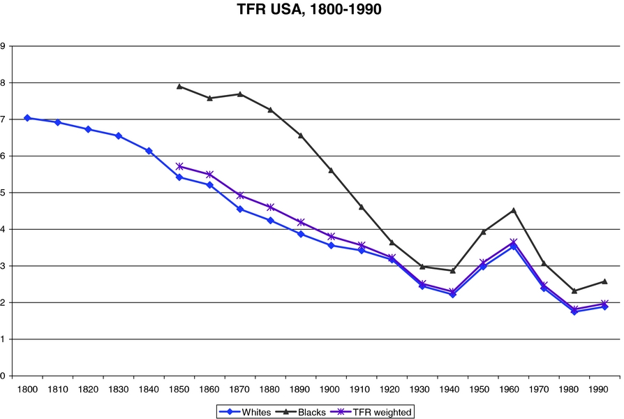
Figure 1. TFR in the USA: 1800–1990.
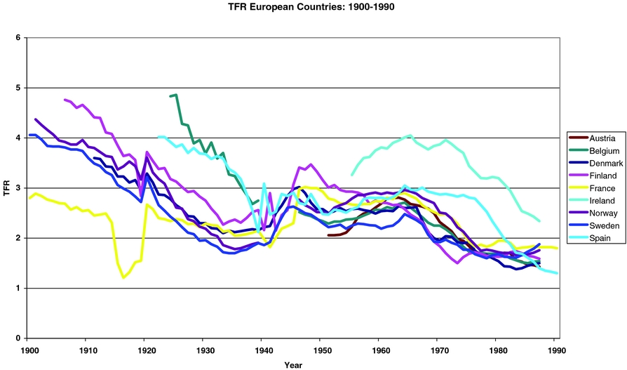
Figure 2. TFR’s in Europe: 1900–1990.
Fact 1: Both in Europe and in the US fertility rates, as measured by the TFR, have decreased constantly over most of the 20th century. The total variation over the 50-year period 1950–2000 is about 1.3 children per woman in Europe, where it has fallen from about 2.8 to about 1.5, and about 1.0 in the US, where it has fallen from about 3.0 to about 2.0.
Fact 2: While in 1920 the average TFRs in Europe and the US were roughly equal, in 2000 they are about 0.4–0.8 children apart (depending on country); the TFR in the US is at 2.0 children per woman, while in Europe it is between 1.2 and 1.6 children per woman.
There are several other relevant facts to keep in mind when interpreting these differences in the historical patterns of fertility in the US and Europe. In the demographic literature, two factors are usually treated as the main driving forces behind long run movements in fertility: reductions in infant mortality rates (IMR) and increases in Female Labor Force Participation Rates (FLFPR).
While IMR might be reasonably thought of as exogenous in individual fertility decisions, labor force participation is clearly endogenous to household decisions. As such, any explanation of variations in TFR based on variations in FLFPR only begs for the common factor(s) affecting both. Leaving this objection aside, it is also clear from the data that the facts cannot be accounted for on the basis of the correlation between TFR and FLFPR. While it is true that FLFPRs have increased over time in both Europe and the US, this has occurred at very different rates. Moreover, over the 1980s and 1990s the cross-country correlation between TFR and FLFPR has turned positive instead of negative (Adsera, Reference Adsera2004). In particular, current LFPRs are higher in the U.S. than in Europe, while TFRs are lower in Europe. Thus, while the time series changes in TFRs in each individual country are consistent with an increase in FLFPR and a negative correlation between TFR and FLFPR this explanation alone cannot account for the cross-sectional evidence. Indeed, the cross-sectional evidence would require the opposite correlation.
Similar, even if less extreme, problems arise with the IMR. The separate time series behavior of TFRs in Europe and the US are consistent with the observed drop in IMR; the respective drops in IMR were from 37/1000 for the U.S. to about 7/1000 (from 1950 to 2000) and, from values between 22/1000 and 60/1000 (depending on the country) to values between 4/1000 and 7/1000 in Europe. Taking 0.030 as our point estimate of the correlation between IMR and TFR (which is halfway between the two estimates of Regressions II and IV given below), the observed time series variations in country by country IMR can account for a drop in fertility that ranges from 0.5 (Sweden) to 1.6 (Spain) children per woman. But an elasticity of 0.030 cannot possibly account for the current differences in TFR between the US and Europe, neither now nor fifty years ago. Mortality rates among infants are basically identical on the two sides of the Atlantic these days, and were higher, not lower, in Europe than in the US in the 1950s. Hence, while a reduction in IMRs has certainly played a role, along the lines of, e.g., Boldrin and Jones (Reference Boldrin and Jones2002), in the fertility decline of both the US and Europe, this explanation also has difficulty with the observed cross-sectional differences over this period.
Similar problems arise with other putative explanations, e.g., increases in income per capita, female education levels, or in the degree of urbanization.
Thus, to account coherently for both facts on the basis of changes in factors that are usually associated to long run movements in fertility, appears difficult.
In contrast, the size and timing of the growth in government pension systems correlates well with both the time series and cross-sectional observations: Beginning shortly after WWII the size and relevance of Social Security were roughly the same as in the US and in European countries. Since then, Social Security has grown everywhere, but this increase has been much more dramatic in Europe than in the US. When the system was first introduced in the US, it was quite small—there were about 50 thousand beneficiaries in 1937, and only two hundred thousand in 1940; it is only right after WWII that the system takes off, and in 1950 the number of beneficiaries reached 3.5 million. Thus, as an approximation, the size of the pension system was 0% of labor income in 1935;Footnote 6 currently, tax receipts and payments are approximately 10% of labor income. In Europe, the payments of the systems were also approximately 0% of labor income in 1935, but the growth has been much more dramatic, in some countries pension payments stand as high as 20–25% of labor income. The history of the U.K system lies someplace in between; for details compare the historical section of the chapters in Gruber and Wise (Reference Gruber and Wise1999) dedicated to European countries.
We would be remiss if we did not point out the anomalous behavior of fertility rates during the 1920–1950 period both in Europe and in the US (where the changes are larger). In both, measured TFR, which had been steadily decreasing since 1800 in parallel with the decrease in IMR and the increase in urbanization, took a sharp swing downward around 1920, reaching particularly low levels during the 1930–1940 decade. Fertility snapped back to much higher levels (about 50% higher, in fact) during the “baby boom” period—1940–1960—after which it decreased again to the current low levels.Footnote 7 Both of these movements are hard to account for on the basis of movements in the standard variables used by demographers to track long fun movements in fertility (IMR, urbanization, female education, and the other, assorted socioeconomic variables used in empirical studies). Thus, although explaining the whole 1920–1960 fertility ” swing” is a fascinating and challenging task, it will not be taken up here.Footnote 8
2.2. Cross-Sectional Data
The loose, but suggestive, discussion of the relative sizes and timing of changes in government pension systems in Europe and the US and their relationship to observed changes in fertility given above is further strengthened by an examination of cross-sectional evidence. We examine a cross section of 104 countries taken from 1997. The raw data are shown in Figure 3.
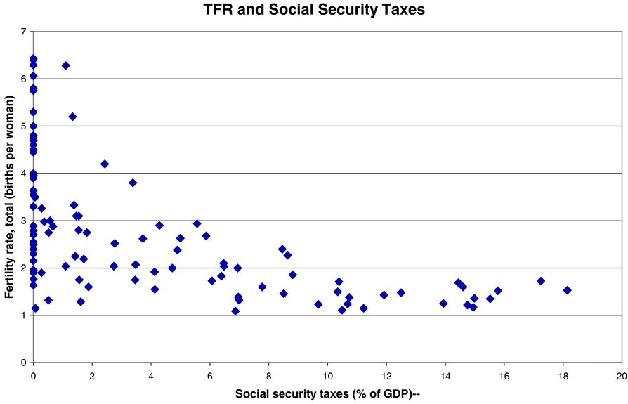
Figure 3. Cross-country correlation, social security tax and TFR.
Although one must be careful about causal interpretations, the data in cross section show a strong negative relationship between the TFR in a country and the size of its Social Security and pension system. This plots TFR for the country in 1997 versus Social Security expenditures as a fraction of GDP in 1997, denoted SST, for these countries. Since this second variable is a measure of the average tax rate for the Social Security system as a whole, we identify it with the SST in what follows. Although the relationship is far from perfect, as can be seen, there is a strong negative relationship between these two variables. Most notably, there are only four countries for which SST is at least 6% and TFR is above 2 (children per woman).Footnote 9
In contrast to this, in those countries where TFR is above three, none has an SST above 4%. This is suggestive of the overall relationship between these two variables. Regression results from this data set confirm and quantify the visual impression, as summarized in the table below.Footnote 10 For cross-section regressions, the dependent variable is TFR, SST is the Social Security tax rate estimated as total expenditures on the Social Security system as a fraction of GDP (in 1997), GDP is per capita GDP in 1995 (in USD 1,000 ), IMR is the Infant Mortality Rate, estimated as the number of deaths per 1,000 live births (in 1997).
As can be seen, the coefficient on SST is negative and highly statistically significant. It is also economically significant. Most LDCs (Lesser Developed Countries) have either no Social Security system or a very small one. In contrast, SST is between 7% and 16% for most developed countries, but only European countries have ratios above 10%. Thus, the relevant range for calculations is in changes in SST from 0% (0.00) to 10% (0.10). Our regressions imply that, everything else the same, an increase in SST of this size (i.e., from 0% to 10%) is associated with a reduction in the number of children per woman of between 0.7 and 1.6. In Regression II, we include two other variables that might either give alternative explanations for the results in column I or allow for a sharper estimation of the conditional correlation between SST and TFR. They are per capita GDP and IMR. Although the size and significance of SST do fall somewhat, it remains substantially negative and statistically significant, while the coefficient on GDP is not significant; the coefficient on IMR has the expected positive sign and is highly significant, which is consistent with the quantitative theoretical predictions of Boldrin and Jones (Reference Boldrin and Jones2002). We also did regressions including education variables from the Barro–Lee data set as additional predictors. The addition of these variables left the coefficient estimates on SST and IMR virtually unchanged and still highly significant. The addition of these variables, while not significant themselves, did increase the size of the GDP coefficient and made it statistically significant.Footnote 11
2.3. A Small Panel Study
We find similar results when we look at panel data. Here, we look at a panel data set of TFRs and SST’s in eight developed countries over the period from 1960 to 2000.Footnote 12 The eight countries are: Austria, Belgium, Denmark, Finland, France, Ireland, Norway, and Spain. A summary of the data are shown in Figure 4 and the regression results are given in Table 1. The columns labeled Regression III and IV show the results of two simple regressions for this panel data set. (Uncorrected for autocorrelation and/or heteroscedasticity.) The variables here have the following meaning: TFR is still TFR in that country/year, SST is the Social Security tax rate measured as Social Security expenditure over labor earnings, IMR is as before, and 65% is the share of the population aged 65 years or older; per capita GDP has been omitted as it is never significant.
Table 1. Fertility and social security, cross section and country panel
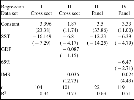
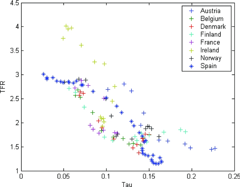
Figure 4. Social security tax and TFR in eight European countries.
The results from this panel regression are qualitatively similar to what we saw above in the cross section—viz., an increase in SST leads to a reduction in TFR, even after controlling for IMR and for the share of elderly people in the population. Quantitative comparisons are more delicate, as the measure for SST adopted here differs from the previous one. Still, if one takes the rough, but overall accurate, approximation that labor earnings are 2/3 of GDP, then an increase in the Social Security expenditure over GDP from 5% to 15% is associated also in the panel data with a fall in TFR of between 1.0 and 1.8 children per woman, similar to the estimates in the cross-section data.
These findings are subject to the same cautions which always accompany regression studies, but they are highly suggestive that SST may indeed have an effect on fertility decisions, that this effect is to reduce the number of children that people have, and that this effect is fairly large in size: an increase of the Social Security system on the order of 10% of GDP is associated with a reduction in TFR of between 0.7 and 1.6 children per woman.
These results are of considerable interest but also must be interpreted with care. In many countries, the Social Security system not only provides old-age insurance (i.e., an annuity) financed with an ad-hoc tax on labor income, but also has an element of forced savings. That is, the benefits paid out to an individual are dependent, to varying degrees in different countries, on the contributions made over the working lifetime of the payee. Because of this, the exact relationship between SST in these regressions and the SST rate in subsequent sections is imperfect. That is, in the models, we will assume that SST is financed through a labor income tax and is paid out lump sum. Thus, from the point of view of testing the model predictions, we would ideally like to have data on that part of SST that most closely mirrors our lump-sum payment mechanism. Data limitations prevent us from attempting this, however. Thus, the effective change in the SST that is relevant for the models is probably smaller than what we have found in the previous regressions.
3. SOCIAL SECURITY IN THE CALDWELL MODEL OF FERTILITY
In this section, we lay out the basic model of children as a parental investment in old age care. In doing this, we follow the development in Boldrin and Jones (Reference Boldrin and Jones2002) quite closely. That is, we assume that there is an altruistic effect going from children to parents, that parents know that this is present, and that they use it explicitly in choosing family size. Thus, the utility of children is increasing in the consumption of their parents, when the latter are in the third and last period of their lives. In our calibration exercise an effort is made to impose a certain degree of discipline on our modeling choice; we use available micro evidence to calibrate the size of the intergenerational transfers in relation to wage and capital income. In modeling the pension system we will make the simplifying assumption that Social Security payments go only to the old and are lump sum. In many real world Social Security Systems, pensions typically have a redistributive component in addition to an annuity structure. We will abstract from these considerations for simplicity. It is likely that, since Social Security systems are a larger fraction of overall wealth for those agents in the lower part of the income distribution, and those individuals also have slightly more children, inclusion of this source of heterogeneity would only increase the size of the effects that we are capturing here.
Our baseline characterization of the Social Security system is therefore one in which pensions are lump-sum, while financing is provided via a payroll tax. Accordingly, let To t denote the transfer received by the old in period t, and let τ t denote the labor income tax rate on the middle aged in period t.
As is standard in fertility models, we will write the cost of children in terms of both goods and labor time components (at
and btwt
, respectively). We assume that labor is inelastically supplied, but that it can be used either for market work or for child-rearing. Thus, total labor income, after taxes is given by (1 − τ
t
)wt
(1 − btnt
), where $n_{t\text{ }}$
denotes the number of young people born at time t. Capital, which in our formulation encompasses all kinds of durable assets, is owned by the old; a fraction of its total value is assumed to be automatically transferred to the middle-aged at the end of the period. We will also assume that the pension system is of the “pay as you go” kind, so that, in equilibrium, To
t
= n
t − 1τ
t
wt
(1 − btnt
). Notice that we use superscripts, y, m, and o to denote, respectively, young, middle-age and old people. Thus, the problem of an agent i, born in period t − 1, i = 1, . . ., n
t − 1, is to:
$n_{t\text{ }}$
denotes the number of young people born at time t. Capital, which in our formulation encompasses all kinds of durable assets, is owned by the old; a fraction of its total value is assumed to be automatically transferred to the middle-aged at the end of the period. We will also assume that the pension system is of the “pay as you go” kind, so that, in equilibrium, To
t
= n
t − 1τ
t
wt
(1 − btnt
). Notice that we use superscripts, y, m, and o to denote, respectively, young, middle-age and old people. Thus, the problem of an agent i, born in period t − 1, i = 1, . . ., n
t − 1, is to:
 \begin{equation*}
Max\ \ U_{t-1}=u(c_{t}^{m})+\zeta u(c_{t}^{o})+\beta u(c_{t+1}^{o}),
\end{equation*}
\begin{equation*}
Max\ \ U_{t-1}=u(c_{t}^{m})+\zeta u(c_{t}^{o})+\beta u(c_{t+1}^{o}),
\end{equation*}
subject to the constraints:
 \begin{eqnarray*}
d_{t}^{i}+s_{t}+c_{t}^{m}+a_{t}n_{t}& \le& (1-\tau _{t})w_{t}(1-b_{t}n_{t}) \\
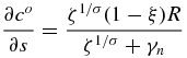
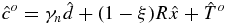
c_{t}^{o}& \le& d_{t}^{i}+\sum _{j\ne i,j=1}^{j=n_{t-1}}d_{t}^{j}+(1-\xi )R_{t}x_{t}+T_{t}^{o}\\
c_{t+1}^{o}& \le& \sum _{j=1}^{j=n_{t}}d_{t+1}^{j}+(1-\xi )R_{t+1}x_{t+1}+T_{t+1}^{o} \\
x_{t+1}& \le& \xi R_{t}x_{t}/n_{t-1}+s_{t}.
\end{eqnarray*}
\begin{eqnarray*}
d_{t}^{i}+s_{t}+c_{t}^{m}+a_{t}n_{t}& \le& (1-\tau _{t})w_{t}(1-b_{t}n_{t}) \\
c_{t}^{o}& \le& d_{t}^{i}+\sum _{j\ne i,j=1}^{j=n_{t-1}}d_{t}^{j}+(1-\xi )R_{t}x_{t}+T_{t}^{o}\\
c_{t+1}^{o}& \le& \sum _{j=1}^{j=n_{t}}d_{t+1}^{j}+(1-\xi )R_{t+1}x_{t+1}+T_{t+1}^{o} \\
x_{t+1}& \le& \xi R_{t}x_{t}/n_{t-1}+s_{t}.
\end{eqnarray*}
Here, cm t is the consumption of a middle aged person in period t, co t is the consumption of an old person, st is the amount of savings, nt is the number of children, di t is the level of support the agent gives to his/her parents, xt is the amount of the capital stock each old person controls in period t, wt is the wage rate, Rt is the gross return on capital in the period, To t is the lump sum transfer received when old, and τ t is the SST rate on labor income. We assume that the decision maker, i, takes dj t , j ≠ i, j = 1, . . ., n t − 1, xt , n t − 1, Rt , R t − 1, and the taxes, To t , To t + 1 and τ t as given. Among other things, this implies that, when choosing a donation level, the representative middle age agent does not cooperate with his own siblings to maximize total utility. Instead, he takes their donations to the parents as given, and maximizes his own utility by choosing a best response level of donations.Footnote 13 Also, note that we have assumed that middle aged individuals work, but that the elderly do not; we do not model here the impact that a Social Security system may or may not have on the life-cycle labor supply of individuals. Notice that we can rewrite the middle age budget constraint as:
 \begin{equation*}
d_{t}^{i}+s_{t}+c_{t}^{m}+\theta _{t}(\tau )n_{t}\le (1-\tau _{t})w_{t},
\end{equation*}
\begin{equation*}
d_{t}^{i}+s_{t}+c_{t}^{m}+\theta _{t}(\tau )n_{t}\le (1-\tau _{t})w_{t},
\end{equation*}
where θ t (τ t ) = at + (1 − τ t )btwt . Since θ t is exogenous to the individual decision maker, using this shorthand will simplify the presentation. In addition to introducing a SST and transfers, we also have deviated from the original Boldrin and Jones paper in that we have included a change in the law of motion of wealth per old person:
 \begin{equation*}
x_{t+1}=\xi R_{t}x_{t}/n_{t-1}+s_{t}.
\end{equation*}
\begin{equation*}
x_{t+1}=\xi R_{t}x_{t}/n_{t-1}+s_{t}.
\end{equation*}
The parameter ξ affords us a simple way of modeling differences, across countries at a given time, and across time in a given country, in both the inheritance mechanisms and the access to financial institutions. This will allow us to study the idea that increased access to financial markets increases the rate of return on private savings to physical capital, which also lessens the value of within-family support in old age, thereby causing fertility to fall. This captures capital depreciation while providing some freedom in our handling of the effective life-time rate of return on wealth accumulation. To do this we proceed as follows. Let 0 < δ < 1 be the depreciation rate per period. Write Rt = (1 − δ)+Fk (K, AL), where F is the aggregate production function, K is capital, L is aggregate labor supply and A is the level of TFP; subscripts denote, here and in what follows, partial derivatives. We will let ξ range in the interval [0, 1]. When ξ = 0 capital markets are fully operational, there are no involuntary or legally imposed bequests, and old people are able to consume the total return from their middle age savings. On the contrary, when ξ = 1, old people have no control whatsoever on their savings, which are entirely and directly passed to the offsprings, whom in turn will be unable to get anything out of them, and so on. In this extreme case, no saving will take place and children’s donations are the only viable road to consumption in old age. As usual, reality fits somewhere in between these two extremes, as discussed in the calibration section.
After substituting in the constraints and using symmetry for donations of future children, this problem can be reformulated as one of solving:
 \begin{equation*}
\max _{s_{t},n_{t},d_{t}}V(s_{t},n_{t},d_{t}),
\end{equation*}
\begin{equation*}
\max _{s_{t},n_{t},d_{t}}V(s_{t},n_{t},d_{t}),
\end{equation*}
where the concave maximand is defined as
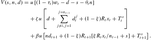 \begin{eqnarray*}
V(s,n,d)& =&u\left[ (1-\tau _{t})w_{t}-d-s-\theta _{t}n\right]\\
&& +\,\zeta u\left[ d+\sum _{j\ne i,j=1}^{j=n_{t-1}}d_{t}^{j}+(1-\xi )R_{t}x_{t}+T_{t}^{o}\right] \\
&& +\,\beta u\left[ nd_{t+1}+(1-\xi )R_{t+1}[\xi R_{t}x_{t}/n_{t-1}+s]+T_{t+1}^{o}\right] .
\end{eqnarray*}
\begin{eqnarray*}
V(s,n,d)& =&u\left[ (1-\tau _{t})w_{t}-d-s-\theta _{t}n\right]\\
&& +\,\zeta u\left[ d+\sum _{j\ne i,j=1}^{j=n_{t-1}}d_{t}^{j}+(1-\xi )R_{t}x_{t}+T_{t}^{o}\right] \\
&& +\,\beta u\left[ nd_{t+1}+(1-\xi )R_{t+1}[\xi R_{t}x_{t}/n_{t-1}+s]+T_{t+1}^{o}\right] .
\end{eqnarray*}
This gives rise to First Order Conditions:Footnote 14
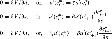 \begin{eqnarray*}
0& =&\partial V/\partial d, \quad \text{or, }\quad u^{\prime }(c_{t}^{m})=\zeta u^{\prime }(c_{t}^{o}) \\
0& =&\partial V/\partial s, \quad \text{or, }\quad u^{\prime }(c_{t}^{m})=\beta u^{\prime }(c_{t+1}^{o})\frac{\partial c_{t+1}^{o}}{\partial s} \\
0& =&\partial V/\partial n, \quad \text{or, }\quad \theta _{t}u^{\prime }(c_{t}^{m})=\beta u^{\prime }(c_{t+1}^{o})\frac{\partial c_{t+1}^{o}}{ \partial n}
\end{eqnarray*}
\begin{eqnarray*}
0& =&\partial V/\partial d, \quad \text{or, }\quad u^{\prime }(c_{t}^{m})=\zeta u^{\prime }(c_{t}^{o}) \\
0& =&\partial V/\partial s, \quad \text{or, }\quad u^{\prime }(c_{t}^{m})=\beta u^{\prime }(c_{t+1}^{o})\frac{\partial c_{t+1}^{o}}{\partial s} \\
0& =&\partial V/\partial n, \quad \text{or, }\quad \theta _{t}u^{\prime }(c_{t}^{m})=\beta u^{\prime }(c_{t+1}^{o})\frac{\partial c_{t+1}^{o}}{ \partial n}
\end{eqnarray*}
A fundamental Rate of Return condition follows immediately from the last two equations; this is:
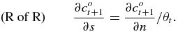 \begin{equation*}
\text{(R of R)}\qquad \frac{\partial c_{t+1}^{o}}{\partial s}=\frac{\partial c_{t+1}^{o}}{\partial n}/\theta _{t}.
\end{equation*}
\begin{equation*}
\text{(R of R)}\qquad \frac{\partial c_{t+1}^{o}}{\partial s}=\frac{\partial c_{t+1}^{o}}{\partial n}/\theta _{t}.
\end{equation*}
Assuming now that u(c) = c 1 − σ/(1 − σ), the three first order conditions can be written in a form which allows for further algebraic manipulation, i.e.
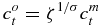 \begin{equation}
c_{t}^{o} =\zeta ^{1/\sigma }c_{t}^{m}
\end{equation}
\begin{equation}
c_{t}^{o} =\zeta ^{1/\sigma }c_{t}^{m}
\end{equation}
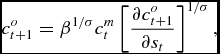 \begin{equation}
c_{t+1}^{o}=\beta ^{1/\sigma }c_{t}^{m}\left[ \frac{\partial c_{t+1}^{o}}{ \partial s_{t}}\right] ^{1/\sigma }\text{,}
\end{equation}
\begin{equation}
c_{t+1}^{o}=\beta ^{1/\sigma }c_{t}^{m}\left[ \frac{\partial c_{t+1}^{o}}{ \partial s_{t}}\right] ^{1/\sigma }\text{,}
\end{equation}
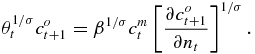 \begin{equation}
\theta _{t}^{1/\sigma }c_{t+1}^{o} =\beta ^{1/\sigma }c_{t}^{m}\left[ \frac{ \partial c_{t+1}^{o}}{\partial n_{t}}\right] ^{1/\sigma }.
\end{equation}
\begin{equation}
\theta _{t}^{1/\sigma }c_{t+1}^{o} =\beta ^{1/\sigma }c_{t}^{m}\left[ \frac{ \partial c_{t+1}^{o}}{\partial n_{t}}\right] ^{1/\sigma }.
\end{equation}
By substituting in the budget constraints and imposing symmetry in the choice of donations (i.e., that dt = dj t ) equation (1) gives:
 \begin{equation*}
n_{t-1}d_{t}+(1-\xi )R_{t}x_{t}+T_{t}^{o}=\zeta ^{1/\sigma }\left[ (1-\tau _{t})w_{t}-d_{t}-s_{t}-\theta _{t}n_{t}\right] .
\end{equation*}
\begin{equation*}
n_{t-1}d_{t}+(1-\xi )R_{t}x_{t}+T_{t}^{o}=\zeta ^{1/\sigma }\left[ (1-\tau _{t})w_{t}-d_{t}-s_{t}-\theta _{t}n_{t}\right] .
\end{equation*}
Solving this for dt gives:
 \begin{equation*}
d_{t}=\frac{1}{\zeta ^{1/\sigma }+n_{t-1}}\left[ \zeta ^{1/\sigma }\left( (1-\tau _{t})w_{t}-s_{t}-\theta _{t}n_{t}\right) -(1-\xi )R_{t}x_{t}-T_{t}^{o}\right] .
\end{equation*}
\begin{equation*}
d_{t}=\frac{1}{\zeta ^{1/\sigma }+n_{t-1}}\left[ \zeta ^{1/\sigma }\left( (1-\tau _{t})w_{t}-s_{t}-\theta _{t}n_{t}\right) -(1-\xi )R_{t}x_{t}-T_{t}^{o}\right] .
\end{equation*}
Using this in the budget constraint for the old, we see that
 \begin{equation*}
c_{t}^{o}=\frac{\zeta ^{1/\sigma }}{\zeta ^{1/\sigma }+n_{t-1}}\left[ n_{t-1}\left( (1-\tau _{t})w_{t}-s_{t}-\theta _{t}n_{t}\right) +(1-\xi )R_{t}x_{t}+T_{t}^{o}\right] .
\end{equation*}
\begin{equation*}
c_{t}^{o}=\frac{\zeta ^{1/\sigma }}{\zeta ^{1/\sigma }+n_{t-1}}\left[ n_{t-1}\left( (1-\tau _{t})w_{t}-s_{t}-\theta _{t}n_{t}\right) +(1-\xi )R_{t}x_{t}+T_{t}^{o}\right] .
\end{equation*}
Thus, after some algebra, we obtain the two rates of return:
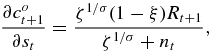 \begin{equation*}
\frac{\partial c_{t+1}^{o}}{\partial s_{t}}=\frac{\zeta ^{1/\sigma }(1-\xi )R_{t+1}}{\zeta ^{1/\sigma }+n_{t}},
\end{equation*}
\begin{equation*}
\frac{\partial c_{t+1}^{o}}{\partial s_{t}}=\frac{\zeta ^{1/\sigma }(1-\xi )R_{t+1}}{\zeta ^{1/\sigma }+n_{t}},
\end{equation*}
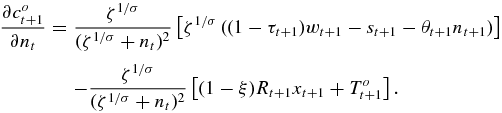 \begin{eqnarray*}
\frac{\partial c_{t+1}^{o}}{\partial n_{t}}& =&\frac{\zeta ^{1/\sigma }}{(\zeta ^{1/\sigma }+n_{t})^{2}}\left[ \zeta ^{1/\sigma }\left( (1-\tau _{t+1})w_{t+1}-s_{t+1}-\theta _{t+1}n_{t+1}\right) \right] \\
&& -\frac{\zeta ^{1/\sigma }}{(\zeta ^{1/\sigma }+n_{t})^{2}}\left[ (1-\xi )R_{t+1}x_{t+1}+T_{t+1}^{o}\right] .
\end{eqnarray*}
\begin{eqnarray*}
\frac{\partial c_{t+1}^{o}}{\partial n_{t}}& =&\frac{\zeta ^{1/\sigma }}{(\zeta ^{1/\sigma }+n_{t})^{2}}\left[ \zeta ^{1/\sigma }\left( (1-\tau _{t+1})w_{t+1}-s_{t+1}-\theta _{t+1}n_{t+1}\right) \right] \\
&& -\frac{\zeta ^{1/\sigma }}{(\zeta ^{1/\sigma }+n_{t})^{2}}\left[ (1-\xi )R_{t+1}x_{t+1}+T_{t+1}^{o}\right] .
\end{eqnarray*}
What remains is to determine the three prices wt , Rt , and θ t from the other endogenous variables. We write feasibility in per old person terms:
 \begin{equation*}
n_{t-1}c_{t}^{m}+c_{t}^{o}+n_{t-1}a_{t}n_{t}+n_{t-1}s_{t}\le Y_{t}=F(x_{t},A_{t}n_{t-1}(1-b_{t}n_{t})),
\end{equation*}
\begin{equation*}
n_{t-1}c_{t}^{m}+c_{t}^{o}+n_{t-1}a_{t}n_{t}+n_{t-1}s_{t}\le Y_{t}=F(x_{t},A_{t}n_{t-1}(1-b_{t}n_{t})),
\end{equation*}
where xt is the amount of capital per old person, and Lt = Atn t − 1(1 − btnt ) is the amount of labor supplied per old person; F is assumed to be CRS. From this, it follows that
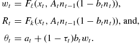 \begin{eqnarray*}
w_{t}& =&F_{\ell }(x_{t},A_{t}n_{t-1}(1-b_{t}n_{t}))\text{,} \\
R_{t}& =&F_{k}(x_{t},A_{t}n_{t-1}(1-b_{t}n_{t}))\text{, and,} \\
\theta _{t}& =&a_{t}+(1-\tau _{t})b_{t}w_{t}\text{.}
\end{eqnarray*}
\begin{eqnarray*}
w_{t}& =&F_{\ell }(x_{t},A_{t}n_{t-1}(1-b_{t}n_{t}))\text{,} \\
R_{t}& =&F_{k}(x_{t},A_{t}n_{t-1}(1-b_{t}n_{t}))\text{, and,} \\
\theta _{t}& =&a_{t}+(1-\tau _{t})b_{t}w_{t}\text{.}
\end{eqnarray*}
Thus, given the initial conditions n − 1, n 0, x 0, the sequence of exogenous variables at , bt , At , τ t , and To t , and the model’s parameters, the full system of equations determining the equilibrium sequences is thereby obtained.
3.1. Exogenous Growth and BGPs
We assume that there is exogenous labor augmenting technological change, At
= γ
t
A
A
0. As it is well known, for there to be balanced growth it must also be that at
= γ
t
A
a
0, bt
= b, and τ
t
= τ. Accordingly we define the de-trended variables in the standard way. That is, $\hat{c}_{t}^{o}=c_{t}^{o}/\gamma _{A}^{t}$
,
$\hat{c}_{t}^{o}=c_{t}^{o}/\gamma _{A}^{t}$
, $\hat{c} _{t}^{m}=c_{t}^{m}/\gamma _{A}^{t}$
,
$\hat{c} _{t}^{m}=c_{t}^{m}/\gamma _{A}^{t}$
, $\hat{d}_{t}=d_{t}/\gamma _{A}^{t}$
,
$\hat{d}_{t}=d_{t}/\gamma _{A}^{t}$
, $\hat{s}_{t}=s_{t}/\gamma _{A}^{t}$
,
$\hat{s}_{t}=s_{t}/\gamma _{A}^{t}$
, $\hat{x}_{t}=x_{t}/\gamma _{A}^{t}$
, and
$\hat{x}_{t}=x_{t}/\gamma _{A}^{t}$
, and $\hat{T}_{t}^{o}=T_{t}^{o}/\gamma _{A}^{t}$
. Finally, we denote nt
/n
t − 1 = γ
nt
. Under our assumptions, if
$\hat{T}_{t}^{o}=T_{t}^{o}/\gamma _{A}^{t}$
. Finally, we denote nt
/n
t − 1 = γ
nt
. Under our assumptions, if $\hat{x}_{t}$
,
$\hat{x}_{t}$
, $\hat{s }_{t}$
, and γ
nt
converge to constants then, so do
$\hat{s }_{t}$
, and γ
nt
converge to constants then, so do $\hat{w}_{t}$
, Rt
, and
$\hat{w}_{t}$
, Rt
, and $\hat{\theta }_{t}$
and, consequently, the equilibrium quantities. The balanced growth equations that these must satisfy are given by:
$\hat{\theta }_{t}$
and, consequently, the equilibrium quantities. The balanced growth equations that these must satisfy are given by:
 \begin{equation}
\hat{c}^{o}=\zeta ^{1/\sigma }\hat{c}^{m}
\end{equation}
\begin{equation}
\hat{c}^{o}=\zeta ^{1/\sigma }\hat{c}^{m}
\end{equation}
 \begin{equation}
\hat{c}^{o}=\frac{\beta ^{1/\sigma }}{\gamma _{A}}\hat{c}^{m}\left[ \frac{ \partial c^{o}}{\partial s}\right] ^{1/\sigma }
\end{equation}
\begin{equation}
\hat{c}^{o}=\frac{\beta ^{1/\sigma }}{\gamma _{A}}\hat{c}^{m}\left[ \frac{ \partial c^{o}}{\partial s}\right] ^{1/\sigma }
\end{equation}
 \begin{equation}
\hat{c}^{o}=\left[ \frac{\beta }{\hat{\theta }\gamma _{A}^{(\sigma -1)}} \right] ^{1/\sigma }\hat{c}^{m}\left[ \frac{\partial c^{o}}{\partial n} \right] ^{1/\sigma }
\end{equation}
\begin{equation}
\hat{c}^{o}=\left[ \frac{\beta }{\hat{\theta }\gamma _{A}^{(\sigma -1)}} \right] ^{1/\sigma }\hat{c}^{m}\left[ \frac{\partial c^{o}}{\partial n} \right] ^{1/\sigma }
\end{equation}
 \begin{equation}
\frac{\partial c^{o}}{\partial s}=\frac{\zeta ^{1/\sigma }(1-\xi )R}{\zeta ^{1/\sigma }+\gamma _{n}}
\end{equation}
\begin{equation}
\frac{\partial c^{o}}{\partial s}=\frac{\zeta ^{1/\sigma }(1-\xi )R}{\zeta ^{1/\sigma }+\gamma _{n}}
\end{equation}
 \begin{equation}
\frac{\partial c^{o}}{\partial n}=\frac{\zeta ^{1/\sigma }}{(\zeta ^{1/\sigma }+\gamma _{n})^{2}}\left[ \zeta ^{1/\sigma }\left( (1-\tau )\hat{w }-\hat{s}-\hat{\theta }\gamma _{n}\right) -(1-\xi )R\hat{x}-\hat{T}^{o}\right]
\end{equation}
\begin{equation}
\frac{\partial c^{o}}{\partial n}=\frac{\zeta ^{1/\sigma }}{(\zeta ^{1/\sigma }+\gamma _{n})^{2}}\left[ \zeta ^{1/\sigma }\left( (1-\tau )\hat{w }-\hat{s}-\hat{\theta }\gamma _{n}\right) -(1-\xi )R\hat{x}-\hat{T}^{o}\right]
\end{equation}
 \begin{equation}
\hat{c}^{m}=(1-\tau )\hat{w}(1-b\gamma _{n})-\hat{a}\gamma _{n}-\hat{d}-\hat{ s}
\end{equation}
\begin{equation}
\hat{c}^{m}=(1-\tau )\hat{w}(1-b\gamma _{n})-\hat{a}\gamma _{n}-\hat{d}-\hat{ s}
\end{equation}
 \begin{equation}
\hat{c}^{o}=\gamma _{n}\hat{d}+(1-\xi )R\hat{x}+\hat{T}^{o}
\end{equation}
\begin{equation}
\hat{c}^{o}=\gamma _{n}\hat{d}+(1-\xi )R\hat{x}+\hat{T}^{o}
\end{equation}
 \begin{equation}
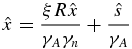
\hat{x}=\frac{\xi R\hat{x}}{\gamma _{A}\gamma _{n}}+\frac{\hat{s}}{\gamma _{A}}
\end{equation}
\begin{equation}
\hat{x}=\frac{\xi R\hat{x}}{\gamma _{A}\gamma _{n}}+\frac{\hat{s}}{\gamma _{A}}
\end{equation}
 \begin{equation}
\hat{w} =F_{\ell }(\hat{x},A_{0}\gamma _{n}(1-b\gamma _{n}))\text{,}
\end{equation}
\begin{equation}
\hat{w} =F_{\ell }(\hat{x},A_{0}\gamma _{n}(1-b\gamma _{n}))\text{,}
\end{equation}
 \begin{equation}
R =(1-\delta )\;+F_{k}(\hat{x},A_{0}\gamma _{n}(1-b\gamma _{n}))\text{,}
\end{equation}
\begin{equation}
R =(1-\delta )\;+F_{k}(\hat{x},A_{0}\gamma _{n}(1-b\gamma _{n}))\text{,}
\end{equation}
 \begin{equation}
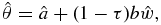
\hat{\theta } =\hat{a}+(1-\tau )b\hat{w}\text{,}
\end{equation}
\begin{equation}
\hat{\theta } =\hat{a}+(1-\tau )b\hat{w}\text{,}
\end{equation}
 \begin{equation}
\hat{T}^{o} =\gamma _{n}\tau \hat{w}(1-b\gamma _{n})\text{.}
\end{equation}
\begin{equation}
\hat{T}^{o} =\gamma _{n}\tau \hat{w}(1-b\gamma _{n})\text{.}
\end{equation}
Simple manipulations give the following expression for the growth rate of population:
 \begin{equation*}
\gamma _{n}=\zeta ^{1/\sigma }\left( \frac{\beta (1-\xi )R}{\gamma _{A}^{\sigma }\zeta }-1\right).
\end{equation*}
\begin{equation*}
\gamma _{n}=\zeta ^{1/\sigma }\left( \frac{\beta (1-\xi )R}{\gamma _{A}^{\sigma }\zeta }-1\right).
\end{equation*}
From the above equation it is clear that steady state fertility only depends on the preference parameters ζ, β, and σ, the exogenous rate of growth of technological progress γ A , the equilibrium interest rate, R, and the degree of capital market imperfection ξ. This implies that the other parameters, such as the costs of having children or the size of the Social Security system, impact steady state fertility only indirectly, through general equilibrium effects embedded in the interest rate. Therefore, in small closed economies, or in economies with a linear technology and fixed prices, there would be no such effects. Most notably, fertility would be invariant to both the size of the Social Security system and the costs of having children. The Barro and Becker model of fertility, as shown in the Appendix, displays a similar feature. In both models, the effects of Social Security on fertility come from general equilibrium effects.
Increasing ξ corresponds to forcing the old to pass on more of their savings to their children and thus represents reducing access to capital markets. This has a direct effect on the growth rate of population as can be seen. Surprisingly, holding R constant and increasing ξ causes γ n to fall, the opposite of what one would expect. There is also an indirect effect of a change in ξ on R. A careful examination of the rate of return condition shows that the indirect effect goes in the opposite direction. In fact, due to the general equilibrium equalization of the rate of return on saving with the rate of return on fertility, an increase in ξ leads to lower investment in physical capital and, hence, a higher value of R in equilibrium. Because of these offsetting effects, the overall impact of more efficient capital markets on the value of (1 − ξ)R and, hence, on the growth rate of population depends on parameters. In Section 6, below, we find that the overall effect is negative as would be expected.
The detailed analysis of Social Security in the Barro and Becker model is presented in the Appendix. As with the Caldwell model, it turns out that any effects on steady state fertility from changes in the size of a PAYGO Social Security system must come through indirect effects working off changes in the equilibrium interest rate.
In sum then, neither of the two models delivers an explicit and unambiguous prediction about the direction of the effect of the introduction of a PAYGO Social Security system on fertility and the growth rate of population. Thus, any effect can only be identified through a more thorough, quantitative exercise. This is what we turn to next.
4. CALIBRATION
In this section, we present quantitative comparative statics results for calibrated versions of the two models. We start by calibrating the model economies to match some key facts of the US economy in 2000. We have also done extensive sensitivity analysis with respect to all of the parameter values. We have found that our key conclusions are the same for a wide range of parameter values, but they are sensitive to the calibration of utility function parameters; we discuss this at the end. Throughout, we assume that a period is 20 years; this choice distorts some of the model’s predictions as it implies that, over the life cycle, the number of working and retirement years is the same, whereas they stand in a ratio of 2 to 1 in reality. For the Caldwell model we consider the case where financial markets are frictionless, ξ = 0. The impact of ξ > 0 on fertility will be considered in the section on Sensitivity Analysis, below.
4.1. Functional Forms
Utility
Recall from Section 3 that for the Caldwell model, the period utility function is assumed to be given by:
 \begin{equation*}
u(c_{t}^{m},c_{t}^{o},c_{t+1}^{o})=\frac{({c_{t}^{m}})^{1-\sigma }}{1-\sigma }+\zeta \frac{({c_{t}^{o}})^{1-\sigma }}{1-\sigma }+\beta \frac{({c_{t+1}^{o} })^{1-\sigma }}{1-\sigma }.
\end{equation*}
\begin{equation*}
u(c_{t}^{m},c_{t}^{o},c_{t+1}^{o})=\frac{({c_{t}^{m}})^{1-\sigma }}{1-\sigma }+\zeta \frac{({c_{t}^{o}})^{1-\sigma }}{1-\sigma }+\beta \frac{({c_{t+1}^{o} })^{1-\sigma }}{1-\sigma }.
\end{equation*}
Production
We assume that the production function is CRS with constant depreciation, and is given by:
 \begin{equation*}
(1-\delta )K+F(K,L)=(1-\delta )K+AK^{\alpha }L^{1-\alpha }.
\end{equation*}
\begin{equation*}
(1-\delta )K+F(K,L)=(1-\delta )K+AK^{\alpha }L^{1-\alpha }.
\end{equation*}
Inputs and output markets are assumed competitive.
4.2. Facts to Match
Setting ξ = 0, there are a total of nine parameters in the Caldwell model.
A number of these parameters are used in macroeconomic models of growth and the business cycle, hence, in calibrating them we follow the existing literature for as many as we can. Accordingly, we normalize A to 1, we set annual depreciation to 8%, and we fix the share of income that goes to capital to either 0.22 or 0.33.Footnote 15 We have set the parameter γ A equal to 1.25% on a yearly basis following Oliveira Peires and Garcia (Reference Oliveira Pires and Garcia2012) estimation for developed countries over the 1970–2000 period, and Dennison’s calculations for the 20th century US.
Additionally, we have made the choice to set the relative weights on the flow utility from current consumption of the old (ζ) to be one for both models. While it makes our life easier, this choice implies, obviously, that on a per capita basis consumption of old parents is equal to that of middle age children. This contradicts the evidence from the empirical life time consumption literature that suggests a drop in all measures of per capita consumption after retirement; estimates of the ratio between average consumption while working and while retired yield values of about 0.70–0.80 . For this ratio to be obtained by co /cm we need to set ζ < 1.0. The impact of this different calibration is also considered in the section on sensitivity analysis, below.
Given these choices, we still need to determine the values of the four parameters β, σ, a, and b. To make our results as clear as possible, for each model we consider two extreme cases: one in which all of the costs of raising children are in terms of goods (b = 0), the other in which they are completely in terms of time (a = 0). This implies calibrating three parameters at a time. The model makes either explicit or implicit predictions about a large number of potentially measurable variables that could be used to help in the calibration: the real rate of return on safe investments, donations as a share of income or consumption, the TFR and the growth rate of the population, the amount of time and/or resources devoted to rearing children, the composition of the population by age group, etcetera. As we must pin down only three parameters we need three independent observations.
To do this, the first step is to choose the country and the historical period the calibrated model is anchored to. Several alternatives are possible, the most obvious choices would be to use data from either the US or Europe at some point in time before government pension programs took off. The US Social Security Administration was created in 1935, thus it would seem natural to calibrate to the US in 1935. However, the period 1930–1950 is also characterized by two anomalous events—the second World War and the Great Depression. In principle both events might have had a major impact on fertility rates, and they certainly had large impacts on the capital–output ratio, measured TFP, and the rate of return on capital; the latter are all relevant macro variables we are taking into consideration to calibrate our model. For these reasons, we calibrate the model to observations from 2000. Because the US is much more homogeneous than Europe, and because we have already set a number of model’s parameters on the basis of US observations, our calibration benchmark is the US in year 2000.
The independent observations we aim at matching are the TFR, the capital–output ratio, and the childbearing costs. In the US the TFR was at 1.75 in 1980, at 2.03 in 1990, and it is around 2.06 currently. Thus, we will take a TFR of 2.00 to be the current “steady-state” level. From Maddison (Reference Maddison1995a, b) we take the capital to output ratio to be between 2.4 and 2.5. We also need to have an estimate of the cost of raising a child. Focus first on the case in which this cost is entirely in time, i.e., a = 0, and b > 0. For this, we set b to be 3% of the available family time, which corresponds to roughly 6% of the mother’s time per child. When total fertility is about 2.0 children per woman this number is consistent with the estimates on time-use data reported by Juster and Stafford (Reference Juster and Stafford1991), with the one estimated by Echevarria and Merlo (Reference Echevarria and Merlo1999) using data fitted to an international cross section, and also with the estimates reported by Moe (Reference Moe1998) based on Peruvian micro data. This number (b = 3%) may seem surprisingly low, in fact the opposite is true. In our context, the fraction b is applied to the total time available for work during the whole working life, while the 6% of mother’s time per child reported in the quoted studies refers only to the infancy-childhood years, which are generally substantially fewer than the active years of a mother. From this point of view, then, a value of b between 2% and 2.5% may be more appropriate; again, we refer to the sensitivity analysis section for this case.
Finally, the parameters describing the Social Security system must be chosen for the model. The exact form of the US Social Security system is much more complex than what we allow for here. Payments received depend, to some extent, on what was paid in and are therefore not exactly lump-sum. Figure 5 shows the time paths of both receipts and expenditures of the Social Security system from 1937 to date. These figures include both Social Security and Medicare, but omit Social Security Disability Insurance since this is not restricted to the elderly. As can be seen these are approximately 7% of GDP over the last two decades of the 20th century. Since labor’s share in income is 67% in the model, this corresponds to an average labor income tax rate of approximately 10%, and this is the value we used in the calibration.
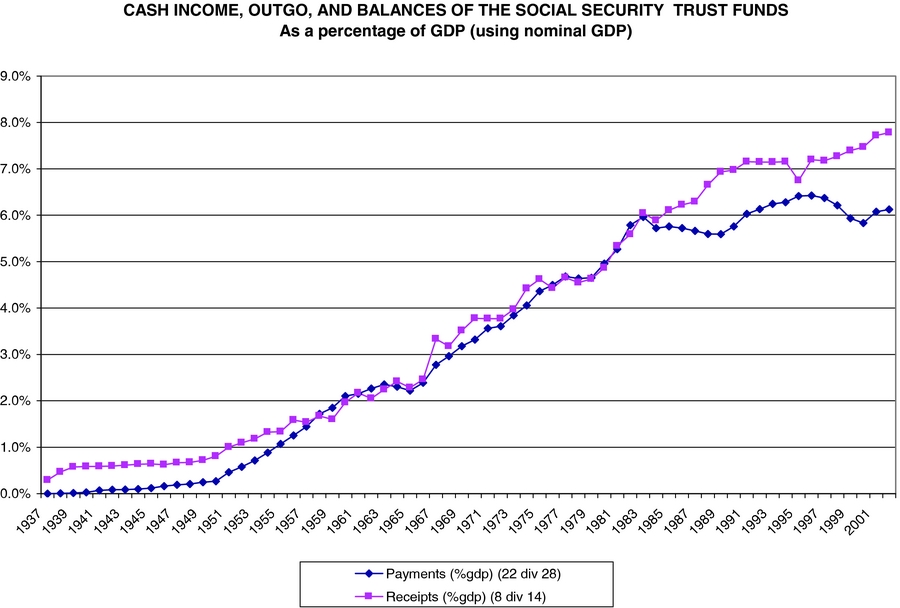
Figure 5. Social security receipts and expenditures/GDP: 1937–2004.
Given this discussion, we will adopt the following three target values for our calibration for the year 2000, when τ = 10%:
-
a. capital–output ratio: 2.4 (annual basis),
-
b. the TFR: 2.0 children per woman, and,
-
c. the amount of time allocated to rearing children: 3% of family time per child.
The model has trouble matching these targets perfectly.Footnote 16 When ζ = 1.0, the elasticity of intertemporal substitution in consumption plays a very secondary role. Our choice of σ = 0.95 and β = 0.99 (yearly) yields a TFR of 1.82 (lower than the targeted value of 2.00) and an annual capital–output ratio of about 2.4 when τ = 0.10 . These two choices together imply an interest rate of about 2.9% per year, perhaps a bit on the low side, when α = 0.33.Footnote 17 For the case in which the time cost (b) is zero, we keep all other parameters the same and we set the good cost of rasing children (a) so that the resulting good cost of raising children as a fraction of per-capita output turns out to be 4.5%. This is a value for which we have a hard time finding real-world estimated counterparts, so we picked it only because it was consistent with observed TFR, capital/output ratios and interest rates at τ = 0.10 when all other calibrated parameters remained the same as above.
The parameter values used in the baseline calibration are summarized in Table 2.
Table 2. Model parameters
5. QUANTITATIVE EFFECTS
In this section, we perform comparative statics by changing the payroll tax over the interval from 0% to 30%, a number consistent with the total employee and employer Social Security contributions in most European countries. We compare our results with the data discussed in Section 2 to see how well the model “fits” the observed patterns of fertility identified there. We discuss:
-
1. For a representative subset of European countries and the US, how much of the variation in fertility that took place during the 1950–2000 period can be accounted for by the growth of the national pension system?
-
2. How much of the persistent US–Europe difference in fertility levels of recent years can be accounted for by the differences in the size of their public pension systems?
-
3. How well do the model predictions compare with our cross-sectional and panel regression results?
We report here results for the Caldwell model, with perfect capital markets. The corresponding results for the Barro and Becker model, which turn out to be quantitatively quite small, are reported in the Appendix.
5.1. Basic Steady State Calculations
Each of the three questions raised above is addressed by comparing steady state calculations of fertility changing only the labor income tax rate used to finance the pension system (with a corresponding, period-by-period balanced budget change in lump sum transfers.) For this reason, we begin by presenting and discussing the basic calculations of comparative steady states that the model implies at our calibrated parameter values.
We begin by examining the case in which there are only time costs of having children. The figures graph different BGP values for a given variable as a function of the SST rate. Figures 6–10 plot, in order, the values of γ n , K/Y, cm /y and co /y Footnote 18 , s/y and d and nd corresponding to the values of τ on the horizontal axis.
Figure 6. Fertility and the SS tax, Caldwell model.
Figure 7. Capital output ratio and the SS tax, Caldwell model.
Figure 8. Consumption of O’s and M’s and the social security tax, Caldwell model.
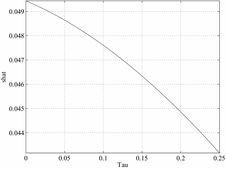
Figure 9. Savings and the social security tax, Caldwell model.
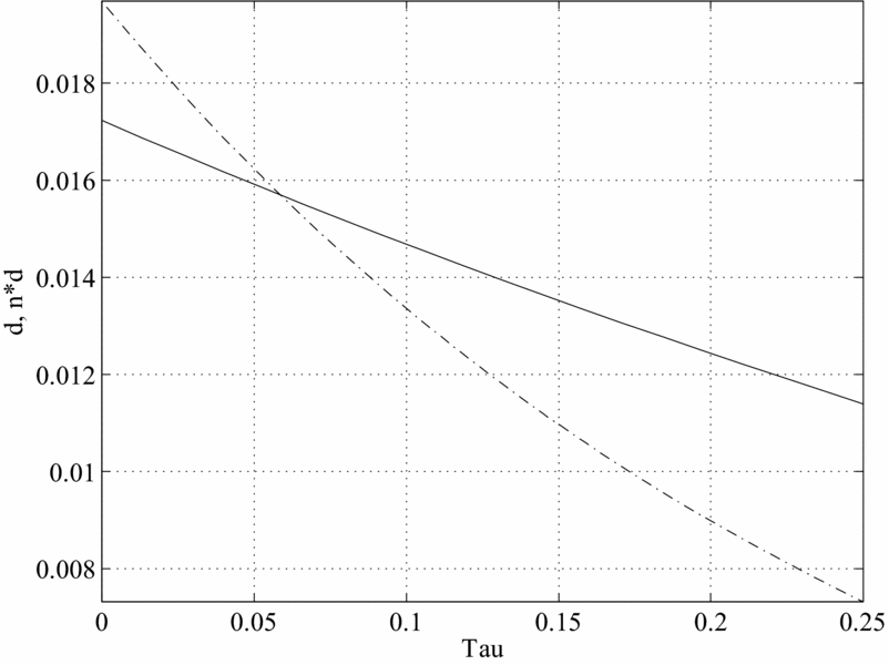
Figure 10. Old age support and the SS tax, Caldwell model.
As we can see, in this framework when the SST moves from 0% to about 10%, the number of children decreases from about 1.15 to about 0.91 (0.9 if there are only goods costs to raising children), the capital–output ratio increases from about 2.2 to 2.4, and there is a sizeable decline in consumption of about 3.0% for both middle aged and old. Finally, donations (both total and per-child) and savings also decrease. The drop in output caused by the introduction of Social Security is large, roughly a 10% deviation from the undistorted BGP level. This drop is larger than that for savings, generating an increase in the capital–output ratios. The drop in fertility is also large as it is equivalent to 0.48 children per woman. When the SST is moved further to about 20–25%, the number of children decreases further to about 0.62–0.65, the capital–output ratio increases to 2.7–2.8 and per-capita consumption also decreases further.
5.2. Comparisons to the Data
Comparisons between Europe and the US, and across time
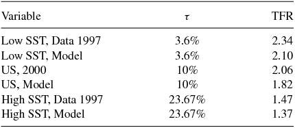
Comparing this to US and European data reported in Sections 1 and 2, we see that the drop predicted by the model is equal to 50% of the observed total drop in TFR between 1950 and 2000; the latter was about equal to one child per woman in the US and 1.3 children per woman in Europe.
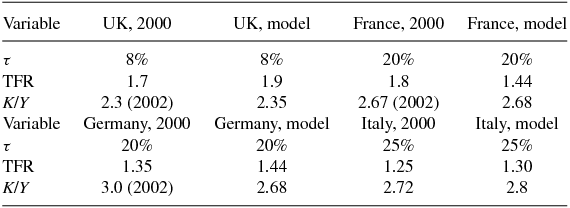
Recall the basic facts that we want to examine. These are that in the US the TFR was about 3.0, and in Europe approximately 2.6, in 1950. At this time, the SST rate was approximately τ = 1% in both regions. By 2000, the SST rate in the US had climbed to around 10% while TFR fell to approximately 2.0. In Europe, both τ and TFR depend on the country, but the relevant range for τ is from around 20% (e.g., France or Germany) to 25% (Italy).
The model predictions for these quantities are contained in Tables 3 and 4.
Table 3. Model and Data, US 1950, and 2000
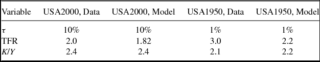
Table 4. Model and data, Europe in 2000
As can be seen in Table 3, the predicted value for TFR for the US is slightly low; 1.82 at τ = 10%, versus the targeted value of 2.0. This was discussed in the section on calibration, and is something that is true for all of the calculated values of TFR from the model. The model predicts that in 1950 fertility should have been 2.2 in both the US and in Europe, substantially lower than the actual value of 3.0 in the US and 2.6 in Europe. But, the predicted change in TFR is 0.38 children per woman or about 40% of the actual difference seen in the US data.
The relevant comparisons for countries like France and Germany with SST rates of τ = 20% are 1.44 for 2000, and 2.2 in 1950. (Here we use the value τ = 1% for 1950.) Again, the model predictions are systematically too low but as can be seen the predicted change in fertility is 2.2 − 1.44 = 0.76 children per woman. This is 50–60% of the observed drop in fertility, depending on the country. Further increasing τ to 25%, the value for Italy, we can see that the model predicts TFR to be 1.30, just slightly above the actual value, and about 75% of the observed change over the 1950 to 2000 period.
As far as comparisons between the US and Europe are concerned, the relevant comparison is between τ = 10% and τ ∈ [20%, 25%]. As can be seen, this implies a difference in TFRs of 1.92 − 1.37 = 0.55 children, comparable to the differences actually seen.
Comparison to the Regression Results of Section 2
Finally, using the cross section of countries studied in Section 2 we constructed two subgroups of countries, one with “large” Social Security systems, one with small.Footnote 19
From these groups, see Table 5, we can see that the changes predicted by the model are roughly in line with what is seen in the data. Indeed, the size of fertility difference predicted from the model when moving from the low SST group to the high SST group is 0.73 children per woman, while that in the data is 0.87 children per woman. With respect to the cross-section regressions presented earlier on, notice that the low SST group has, roughly, the same IMR rate as the high SST group but much lower values for the 65% variable: the range is 4.6–11.5, averaging at 7.9%, versus a range of 13.5–17.5 averaging at 15.8% for the high SST group. We should, however, compare our results also to what we found in our econometric estimates; there, once we control for infant mortality and the fraction of the population over 65, a 20% increase in the SST is associated with a drop in TFR of between 1.3 and 2.4 children per woman. Thus, our model accounts for between 30% and 55% of the observed differences in fertility in the overall cross section.
Table 5. Model and data for three groups of countries
In the Caldwell-type framework, the quantitative effects of changes in the size of the Social Security system are similar for the two alternative cost structures (time costs and goods costs). This is because in this framework the key mechanism governing fertility is how fertility translates into transfers to parents, and how sensitive these are to changes in the number of children. The introduction of a Social Security system reduces per-child donations, and hence fertility. The difference between the two is in the distortionary effect of taxation on the child-rearing versus market activities. If the costs of children are solely in terms of goods, in this framework with inelastic labor supply, there is no offsetting substitution effect when τ is increased. Thus, the effects on fertility are larger, if only slightly, in this case.
As an additional dimension along which the two models’ predictions should be compared, we note that the Caldwell-type model predicts an increase in the capital–output ratio, while the Barro and Becker model predicts a decrease of the capital–output ratio as Social Security increases. In the data, the US capital–output ratio has either remained constant or increased since early in the 20th century; also, the capital–output ratio is substantially higher among the European countries, relative to the US, and the European countries have, with the sole exception of the UK, a substantially higher SST than the US. This lends further empirical support to Caldwell-type models of fertility as an alternative to dynastic models.
6. SENSITIVITY ANALYSIS
6.1. Parameters of Preferences and Technology
The long and the short of the sensitivity analysis results is: varying preference parameters within reasonable intervals does not change the qualitative predictions of the two models, nor the magnitude of Δγ n /Δτ as a percentage of the initial value of γ n . It is still and uniformly true that increasing τ from about 0% to 10% decreases TFR by between 20% and 25% in a Caldwell-type model (the corresponding change is slightly less than 1% in the Barro–Becker model—see the Appendix). Similarly, pushing τ from about 10% to 25% decreases TFR by roughly 30% (it is about 5% in the Barro–Becker model).
What varies substantially, and sometimes dramatically, with the preference parameters are the levels of both fertility and the capital–output ratio, and this sensitivity in levels is common to both models.
As illustrated earlier on, at the baseline parameter values the implied TFR is slightly below the current value of 2.06 in the US for the BJ model; for the Barro and Becker model, as shown in the Appendix, the values for b (resp. a) needed to match observations are much larger than the estimated 3% of time. This seems to point to a lack of richness of the models overall. Clearly, however, a model with features of both would do much better. Since the aim of this paper is partially to compare the two models, this was not attempted.
Our findings for changes in the parameters governing technology are similar to those for preferences: small changes in either α, γ A , a, b, or δ bring about changes in fertility and in the capital–output ratio that are sometimes substantial. However, they leave the comparative static results basically unaltered when it comes to fertility. Indeed, in the BJ model, reducing the time cost of children from the b = 3% value adopted in the baseline case to values slightly higher than b = 2% suffices to make the predicted level of fertility to match current averages in the US, i.e. about 2.06 per woman. This choice may be justified by the fact that in our model the effective time cost of having children is artificially increased by the assumption that, with only three periods, the length of working life is equal to that of the retirement period. As explained above, this is a gross distortion of the real world, where the number of years spent working is roughly twice the number of years spent in retirement. Because of this fact, one may argue that b = 2% is a preferable baseline calibration for the BJ-type setting; should this choice be made, our model can easily match current US fertility levels when τ = 10% and the remaining parameters are as in Table 2, without affecting any of the comparative statics results.
One experiment that is of particular interest is the effects of changes in the growth rate of productivity. Our value of 1.012 is fairly low and is based on Dennison’s work, which makes substantial adjustments for the observed changes in labor quality. We also performed our baseline experiments on the effects of changes in τ on γ n for values of γ A up to and including 1.02. These gave rise to very similar results: when the size of the SST increases from 0% to 10% , fertility drops of almost half a child per woman.
Another alteration that is particularly relevant concerns changing α . In the household production literature (which treats the stock of housing and durables as inputs into the production of home goods, and removes the housing service component from GNP) an estimate of α = 0.22 has been found in McGrattan, Rogerson and Wright (Reference McGrattan, Rogerson and Wright1997). Recalibrating the BJ model to this target does not change the overall effects of changes in Social Security on fertility, but it does greatly enhance our ability to hit the targets set out in the previous section. In particular, with α = 0.22, γ n = 1, is attainable even with ζ = 0.65. When this alternative calibration is adopted for the dynastic model, increasing the SST rate still increases fertility, and still only very marginally. In the BJ-type model, increasing the Social Security tax rate reduces fertility of more or less the same percentage as in the base line model.
6.2. The Role of Financial Markets Imperfections
In our version of the BJ model the parameter ξ ∈ (0, 1) measures the extent to which financial market imperfections prevent middle age individuals from using private saving as a means of financing late age consumption. In the baseline model we assumed ξ = 0, so that financial markets are functioning perfectly. As reported in the introduction, a number of empirical studies have found evidence that different measures of the ability to save for retirement are strongly correlated with fertility decisions. In fact, a study by Cigno and Rosati using Italian and German micro data have estimated that the impact of financial market accessibility on fertility is comparable to that of public pensions: the easier it is to save for retirement, the lower is fertility. In the BJ model the intuition for this result is simple: in the equation for the equilibrium donations (see Section 3) the terms (1 − ξ)Rtxt and To t are interchangeable—a variation in ξ has the same effect as a change in the public pension transfer. The more imperfect capital markets are, the less valuable physical capital is for financing consumption in late age and, therefore, the more valuable children are in this regard. One would expect, then, that when ξ > 0 fertility would be higher than in the baseline case; the question is: how much higher?
The answer, reflected in Figure 11, is: a lot higher. Figure 11 plots the mapping from the pair (τ, ξ) ∈ [0.0, 0.25] × [0.0, 0.20] into the equilibrium values of γ n , while Figure 12 has K/Y on the vertical axis and the same two parameters on the horizontal plane. As the reader can verify, even small changes in the efficiency of financial markets make children a very valuable form of investment. This in turn pushes fertility to levels similar to those observed in the earlier part of the 20th century. In quantitative terms, we find that, even in the presence of a Social Security system of roughly the same magnitude as the current one, a reduction in the rate of return on capital of about 20% (ξ = 0.2) would increase fertility 30%, or 0.66 more children per woman in our setting. Equally important, the same degree of financial market inefficiency leads to a substantial decrease in aggregate savings resulting in a K/Y ratio which is almost 50% lower than in the baseline case. These are large effects by historical standards.
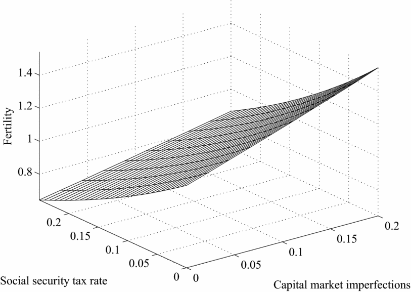
Figure 11. Fertility, social security tax and $\xi$
, Caldwell model.
$\xi$
, Caldwell model.
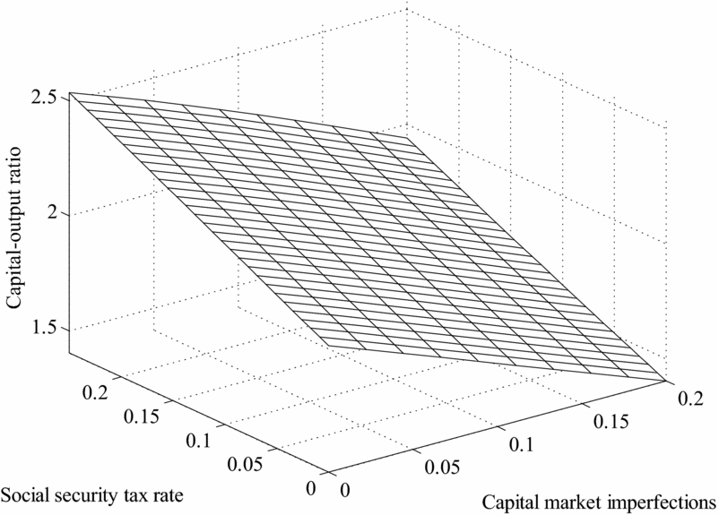
Figure 12. K/Y, social security tax and $\xi$
, Caldwell model.
$\xi$
, Caldwell model.
Financial instruments through which one can reliably save for retirement are limited both historically in the developed countries and currently in the developing countries. It is difficult to know if changing ξ from 0 to 0.2 corresponds to an interesting quantitative exercise without further data work. But, the fact that the effects that we find are so large makes this an interesting possibility to explore further.
7. CONCLUSION
A number of authors have suggested that the welfare state, and the public pension system in particular, might be an important factor behind the drop in fertility to the bare (or even below) replacement levels most western countries are experiencing. Controlling for infant mortality, income level, and female labor force participation, almost all regression exercises, including ours, point to a strong negative correlation between the size of the Social Security system and the TFR, both across countries and over time. In particular, we observe the following: fertility rates were much higher in the US and Europe around 1950, when both groups of countries had a much smaller pension system than they do; since the late 1970s fertility rates have been persistently lower in Europe than in the US, and the former countries have a substantially larger pension system than the latter.
In this paper we test the ability of two models of endogenous fertility to replicate this correlation when they are calibrated to match other very elementary facts of the US economy. The results are mixed. We find that in models based on parental altruism changes in the size of Social Security systems like those we have seen over the last 100 years generate only small (and typically positive) effects on fertility. In contrast, models based on the “old age security” motive for fertility are more in accord with the patterns seen in the data. Although imperfect, even simple, calibrated models of this type account between 40% and 60% of the observed differences in fertility over time in the US or between the US and other developed countries. Since the introduction of government funded pension systems has a much larger effect on incentives at the lower end of the income distribution, this finding is also consistent with the observation that the reduction in fertility over this period has been much larger for poorer households.
In addition to this, we study the effects of improved access to savings instruments on fertility. We find that even small improvements in rates of return (on the order of 20%) have the potential to account for about 50% of the observed changes in fertility over time. This channel is one which requires more exploration, but, apparently it is quite powerful.
Taken together then, we find that these two effects account for between 50% and 100% of the drop in fertility in the US from 3.0 children per woman to 2.0 over the period from 1920 to now.
A. APPENDIX A
A.1. Social Security in the B&B Model of Fertility
In this section, we develop the equations determining the fertility effects of a Social Security system in the BB model. There is a basic problem with trying to study Social Security in a BB model. This is that they assume that people only live two periods, youth and adulthood, and hence there is no time when the middle aged can be taxed to finance consumption of the old. Because of this, we will adapt the model to allow for three period lives. As above, we assume that individuals work when they are middle aged, but do not when they are old. As in this case we want to consider also the impact of a lump sum pension system, let Tm t denote the lump sum tax on the middle age in period t. That is, we will write the problem of the dynasty as choosing Ny t , Nm t , No t , cm t , co t and kt to solve:
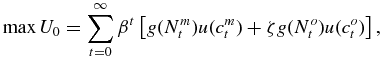 \begin{equation*}
\max U_{0}=\sum _{t=0}^{\infty }\beta ^{t}\left[ g(N_{t}^{m})u(c_{t}^{m})+ \zeta g(N_{t}^{o})u(c_{t}^{o})\right] \text{,}
\end{equation*}
\begin{equation*}
\max U_{0}=\sum _{t=0}^{\infty }\beta ^{t}\left[ g(N_{t}^{m})u(c_{t}^{m})+ \zeta g(N_{t}^{o})u(c_{t}^{o})\right] \text{,}
\end{equation*}
subject to:
 \begin{equation*}
N_{t}^{o}c_{t}^{o}+N_{t}^{m}c_{t}^{m}+N_{t}^{y}(a_{t}+k_{t+1})\le (1-\tau _{t})(N_{t}^{m}-bN_{t}^{y})w_{t}+N_{t}^{m}R_{t}k_{t}+N_{t}^{m}T_{t}^{m}+N_{t}^{o}T_{t}^{o}.
\end{equation*}
\begin{equation*}
N_{t}^{o}c_{t}^{o}+N_{t}^{m}c_{t}^{m}+N_{t}^{y}(a_{t}+k_{t+1})\le (1-\tau _{t})(N_{t}^{m}-bN_{t}^{y})w_{t}+N_{t}^{m}R_{t}k_{t}+N_{t}^{m}T_{t}^{m}+N_{t}^{o}T_{t}^{o}.
\end{equation*}
As above, we let
 \begin{equation*}
\theta _{t}(\tau _{t})=a_{t}+(1-\tau _{t})bw_{t}=a_{t}+b(\tau _{t})w_{t}\text{,}
\end{equation*}
\begin{equation*}
\theta _{t}(\tau _{t})=a_{t}+(1-\tau _{t})bw_{t}=a_{t}+b(\tau _{t})w_{t}\text{,}
\end{equation*}
and use the simplification that
 \begin{equation*}
N_{t}^{o}=N_{t-1}^{m}=N_{t-2}^{y}\text{.}
\end{equation*}
\begin{equation*}
N_{t}^{o}=N_{t-1}^{m}=N_{t-2}^{y}\text{.}
\end{equation*}
Then, we can rewrite this problem as:
 \begin{equation*}
\max U_{0}=\sum _{t=0}^{\infty }\beta ^{t}\left[ g(N_{t}^{m})u(c_{t}^{m})+ \zeta g(N_{t-1}^{m})u(c_{t}^{o})\right] ,
\end{equation*}
\begin{equation*}
\max U_{0}=\sum _{t=0}^{\infty }\beta ^{t}\left[ g(N_{t}^{m})u(c_{t}^{m})+ \zeta g(N_{t-1}^{m})u(c_{t}^{o})\right] ,
\end{equation*}
subject to:
 \begin{equation*}
N_{t-1}^{m}c_{t}^{o}+N_{t}^{m}c_{t}^{m}+N_{t+1}^{m}(\theta _{t}+k_{t+1})\le N_{t}^{m}[(1-\tau _{t})w_{t}+R_{t}k_{t}+T_{t}^{m}]+N_{t-1}^{m}T_{t}^{o}.
\end{equation*}
\begin{equation*}
N_{t-1}^{m}c_{t}^{o}+N_{t}^{m}c_{t}^{m}+N_{t+1}^{m}(\theta _{t}+k_{t+1})\le N_{t}^{m}[(1-\tau _{t})w_{t}+R_{t}k_{t}+T_{t}^{m}]+N_{t-1}^{m}T_{t}^{o}.
\end{equation*}
Since we want to model the Social Security system as transferring money from workers to retirees, we have that Tm t < 0, and To t > 0. Note that we have assumed that although the tax variables, τ t , Tm t , and To t are taken as given, the dynasty head understands that changing Nm t (for example), changes both his tax obligation and his transfer receipts. Hence, even when τ t = 0, this assumption de facto, makes the Social Security system not lump sum, as a distortionary tax and transfer pair (Tm t , and To t + 1) is being applied on the endogenous variable Nm t . An alternative formulation would have the head taking total transfers in each period as given, independently of the fertility choice. Note that, when the total transfer is independent of the dynasty’s fertility choice, a version of Ricardian Equivalence follows immediately if τ t = 0 for all t, and Nm tTt m = −Nm t − 1 Tt o for all t. This is no longer true when Tm t , and To t are given on a per-capita basis, and the dynasty understands that increasing current fertility raises taxes today and transfers tomorrow. In these circumstances a PAYGO pension system may distort fertility choices in either directions, depending on parameter values. To see this notice that, setting τ t = 0 for all t, a simple manipulation of the first order conditions shows that the pension system is neutral if
 \begin{equation*}
-R_{t+1}T_{t}^{m}=T_{t+1}^{0}.
\end{equation*}
\begin{equation*}
-R_{t+1}T_{t}^{m}=T_{t+1}^{0}.
\end{equation*}
It reduces fertility (because it raises the cost of having children) if − R t + 1 Tm t > T 0 t + 1 and it promotes fertility in the opposite case. As the sequences for Tm t , and To t need not be constant, the distortion may go in either direction during different periods. The PAYGO constraint, assuming it treats all dynasties symmetrically, allows one to write the neutrality restriction as
 \begin{equation*}
R_{t+1}N_{t}^{m}T_{t}^{m}=N_{t+1}^{m}T_{t+1}^{m}.
\end{equation*}
\begin{equation*}
R_{t+1}N_{t}^{m}T_{t}^{m}=N_{t+1}^{m}T_{t+1}^{m}.
\end{equation*}
Along a BGP, this means that
 \begin{equation*}
R=\gamma _{N}\gamma _{A}
\end{equation*}
\begin{equation*}
R=\gamma _{N}\gamma _{A}
\end{equation*}
must hold as per capita transfers must grow at the same rate as income per capita grow along a BGP. Dynamic efficiency, though, requires that
 \begin{equation*}
R > \gamma _{N}\gamma _{A}=1+g
\end{equation*}
\begin{equation*}
R > \gamma _{N}\gamma _{A}=1+g
\end{equation*}
as the right-hand side is the growth rate of the aggregate economy. Hence, along dynamically efficient BGPs, lump sum public pensions have a negative direct effect on fertility, and vice versa along dynamically inefficient ones. Notice that, either way, the effect is permanent: everything else the same, a BGP with Tm t , and To t different from zero should have a lower (higher) value for γ N than one without. The result makes economic sense: the pension system we are considering is tantamount to a tax on fertility, at least when R > 1 + g.
To allow for comparison with the old age security model, we now set Tm t = 0, so that To t = Nt m τ t wt (1 − bNm t + 1) is the PAYGO budgetary restriction; to keep as close as possible with the standard Barro–Becker formulation we also assume that g(N) = N η and u(c) = c 1 − σ/(1 − σ).Footnote 20 Retaining the notation from the previous section and assuming the same production function we get (after some algebra) that on a BGP, the system must satisfy:
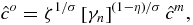 \begin{equation}
\hat{c}^{o} =\zeta ^{1/\sigma }\left[ \gamma _{n}\right] ^{(1-\eta )/\sigma }\hat{c}^{m}\text{,}
\end{equation}
\begin{equation}
\hat{c}^{o} =\zeta ^{1/\sigma }\left[ \gamma _{n}\right] ^{(1-\eta )/\sigma }\hat{c}^{m}\text{,}
\end{equation}
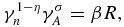 \begin{equation}
\gamma _{n}^{1-\eta }\gamma _{A}^{\sigma } =\beta R\text{,}
\end{equation}
\begin{equation}
\gamma _{n}^{1-\eta }\gamma _{A}^{\sigma } =\beta R\text{,}
\end{equation}
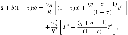 \begin{eqnarray}
\hat{a}+b(1-\tau )\hat{w}& =&\frac{\gamma _{A}}{R}\left[ (1-\tau )\hat{w}+ \frac{(\eta +\sigma -1)}{(1-\sigma )}\hat{c}^{m}\right] \nonumber \\
&& +\frac{\gamma _{A}^{2}}{R^{2}}\left[ \hat{T}^{o}+\frac{(\eta +\sigma -1)}{ (1-\sigma )}\hat{c}^{o}\right],
\end{eqnarray}
\begin{eqnarray}
\hat{a}+b(1-\tau )\hat{w}& =&\frac{\gamma _{A}}{R}\left[ (1-\tau )\hat{w}+ \frac{(\eta +\sigma -1)}{(1-\sigma )}\hat{c}^{m}\right] \nonumber \\
&& +\frac{\gamma _{A}^{2}}{R^{2}}\left[ \hat{T}^{o}+\frac{(\eta +\sigma -1)}{ (1-\sigma )}\hat{c}^{o}\right],
\end{eqnarray}
 \begin{equation}
\hat{c}^{o}+\gamma _{n}\hat{c}^{m}+\gamma _{n}^{2}(\hat{a}+b(1-\tau )\hat{w} +\gamma _{A}\hat{k}) =\gamma _{n}[(1-\tau )\hat{w}+R\hat{k}]+\hat{T}^{o} \text{,}
\end{equation}
\begin{equation}
\hat{c}^{o}+\gamma _{n}\hat{c}^{m}+\gamma _{n}^{2}(\hat{a}+b(1-\tau )\hat{w} +\gamma _{A}\hat{k}) =\gamma _{n}[(1-\tau )\hat{w}+R\hat{k}]+\hat{T}^{o} \text{,}
\end{equation}
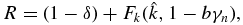 \begin{equation}
R =(1-\delta )+F_{k}(\hat{k},1-b\gamma _{n})\text{,}
\end{equation}
\begin{equation}
R =(1-\delta )+F_{k}(\hat{k},1-b\gamma _{n})\text{,}
\end{equation}
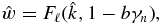 \begin{equation}
\hat{w} =F_{\ell }(\hat{k},1-b\gamma _{n})\text{,}
\end{equation}
\begin{equation}
\hat{w} =F_{\ell }(\hat{k},1-b\gamma _{n})\text{,}
\end{equation}
 \begin{equation}
\hat{T}^{o} =\gamma _{n}\tau \hat{w}(1-b\gamma _{n})\text{.}
\end{equation}
\begin{equation}
\hat{T}^{o} =\gamma _{n}\tau \hat{w}(1-b\gamma _{n})\text{.}
\end{equation}
Comparing equation (17) with the neutrality restriction derived above for the lump-sum case, we can see that, depending on the value of the discount factor β, the general equilibrium effect can push the inequality either way; the same equation also shows, once again, that steady state fertility only depends on the preference parameters η, β, σ, the growth rate of exogenous technological progress γ A and the equilibrium interest rate. Therefore, as in the BJ framework, all other parameters, including the size of the Social Security system, and the costs of having children, only impact fertility indirectly through the interest rate. These effects are thus absent in presence of fixed prices. In sum then, also this model does not deliver an explicit and unambiguous prediction about the direction of the effect of the introduction of a PAYGO Social Security system on fertility and the growth rate of population. Thus, any effect can only be identified through a more thorough, quantitative exercise. This is what we turn to next.
Calibrating the Barro and Becker model
The utility function for the Barro–Becker model is given by:
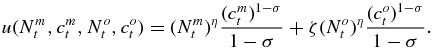 \begin{equation*}
u(N_{t}^{m},c_{t}^{m},N_{t}^{o},c_{t}^{o})=({N_{t}^{m}})^{\eta }\frac{({ c_{t}^{m}})^{1-\sigma }}{1-\sigma }+\zeta ({N_{t}^{o}})^{\eta }\frac{({ c_{t}^{o}})^{1-\sigma }}{1-\sigma }.
\end{equation*}
\begin{equation*}
u(N_{t}^{m},c_{t}^{m},N_{t}^{o},c_{t}^{o})=({N_{t}^{m}})^{\eta }\frac{({ c_{t}^{m}})^{1-\sigma }}{1-\sigma }+\zeta ({N_{t}^{o}})^{\eta }\frac{({ c_{t}^{o}})^{1-\sigma }}{1-\sigma }.
\end{equation*}
As with the Caldwell model we assume that the production function is CRS with constant depreciation, and is given by:
 \begin{equation*}
(1-\delta )K+F(K,L)=(1-\delta )K+AK^{\alpha }L^{1-\alpha }.
\end{equation*}
\begin{equation*}
(1-\delta )K+F(K,L)=(1-\delta )K+AK^{\alpha }L^{1-\alpha }.
\end{equation*}
There are a total of ten parameters in the model, nine of which are in common with the BJ model, while the tenth, η ∈ (0, 1), is specific to the BB model.
We set the parameters of technology as in the BJ model. These include A, δ, α and γ A . Following our choice in the BJ model, we set the relative weights on the flow utility from current consumption of the old (ζ) to be one.
Given these choices, we still need to determine the values of the four parameters β, σ, a, and b, as in the BJ model and we must also choose a value of η. To make our results as clear as possible, for each model we consider two extreme cases: one in which all of the costs of raising children are in terms of goods (b = 0), the other in which they are completely in terms of time (a = 0). This implies calibrating four parameters. Our method for accomplishing this follows closely the description for the BJ model. We choose parameters to match facts for fertility, capital/output ratios from US data in 2000, with τ = 10%.
For ease of comparisons with the results of the BJ model we chose ζ = 1.0, σ = 0.95 and β = 0.99. There are, as mentioned earlier, restrictions on these parameters: σ < 1, and σ + η > 1. Given these restrictions, we were not able to set the time cost of having children anywhere near what one would call “realistic” values while, at the same time, matching a TFR of 2.0 for any value of τ in the relevant range. To match targets for fertility, etc., we must set the time cost of having a child to 33% of the available time. Even then, the parameter η needs to be set as low as possible to keep fertility at a reasonable level in the BB model. When we set b to zero, the level of child care costs that this requires is a = 27% of per capita income.
The parameter values used in the calibration are summarized in Table 6 where we also include the parameter values for the BJ model for comparison.
Table 6. Parameter values for the B&B model
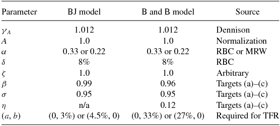
Quantitative effects in the B&B model
Leaving aside the obvious effects on output and wealth that the introduction of a distortionary tax causes, the impact of Social Security on fertility rates in the BB framework is substantially different, almost opposite, from the one we have observed in the data. Figure 13 plots the values taken in the BB model by γ n as τ varies. Indeed, whether fertility increases or decreases in the BB model when Social Security is introduced depends on whether households need mainly goods or time to raise children. If mainly time is needed to raise children, fertility increases as the size of the Social Security program increases, which is the case reported in Figure 13. Notice that the increase is basically insignificant; in the case reported, for example, TFR increases of about 0.05 children as the SST goes from zero to ten per cent. Conversely, if only goods are needed to raise children, the introduction of Social Security decreases the number of children per woman by about 0.014. These effects are orders of magnitude smaller than those seen in the data. The effects on capital accumulation and consumption (of both middle-aged and old) go in the opposite direction, but are also quantitatively small.Footnote 21 The donations effect is missing in this framework, and the different impact on fertility depending on type of cost needed to raise children is due to distortionary taxation: time spend raising children is not taxed, while time spent working is taxed.

Figure 13. Fertility and the social security tax, BB model.
The basic reason for the small effects on fertility in the BB model is that in a balanced PAYGO system, the effects of transfers are netted out by the dynasty planner. Thus, as noted above, if the system was funded entirely through lump sum taxation and its internal rate of return was not dissimilar from the rate of return on capital, the effects would be literally zero. If child-rearing requires time, however, there is a change due to, as discussed above, a change in the effective relative prices of the two uses for time, work and childcare. This effect is typically small, however, and present only if the cost of children is in terms of time, hence the resulting effect on fertility is also small. An additional effect is also present. This is that, even when the costs are entirely in terms of goods, the dynasty views per capita transfers as fixed, whereas in equilibrium, through the government budget constraint, these are determined by average fertility across dynasties. This connection is not recognized by the individual dynasty however, and is the sole reason why, with only goods cost of children, the effect of changes in Social Security are not exactly zero.


