


1. Introduction
Ice discharge from marine outlet glaciers is a function of deformational and basal sliding velocities. It has been suggested that relatively small increases in surface ablation may result in disproportionately large increases in ice discharge via basal sliding (Reference Zwally, Abdalati, Herring, Larson, Saba and SteffenZwally and others, 2002; Reference Bartholomew, Nienow, Mair, Hubbard, King and SoleBartholomew and others, 2010). Recent interferometric synthetic aperture radar (InSAR) observations have confirmed that an annual velocity cycle is spatially widespread in the marginal ice of West Greenland. This annual velocity cycle is most likely due to seasonal changes in basal sliding velocity (Reference Joughin, Das, King, Smith, Howat and MoonJoughin and others, 2008). Recently, however, some studies have speculated that projected increases in surface meltwater production will likely result in a net decrease in basal sliding velocity due to a transition from relatively inefficient to efficient subglacial drainage (Reference SchoofSchoof, 2010;Reference Sundal, Shepherd, Nienow, Hanna, Palmer and HuybrechtsSundal and others, 2011). This motivates the need to quantitatively address the physical relation between glacier hydrology and basal sliding velocity. We therefore seek a computationally efficient means of reproducing the observed spatial and temporal patterns of basal sliding so that we can ultimately explore the likely response of outlet glacier dynamics to climate change scenarios. Other observations and models indicate that the ice discharge from Greenland’s marine-terminating glaciers is highly sensitive to calving-front perturbations, which are subsequently propagated upstream via longitudinal coupling (Reference Holland, Thomas, de Young, Ribergaard and LyberthHolland and others, 2008; Reference Joughin, Das, King, Smith, Howat and MoonJoughin and others, 2008; Reference Nick, Vieli, Howat and JoughinNick and others, 2009). We also explore this alternative mechanism as a cause for the observed annual velocity cycle.
The Sermeq Avannarleq ablation zone in West Greenland exhibits an annual ice velocity cycle similar to that of an alpine glacier. The critical features of this cycle are a summer speed-up event followed by a fall slowdown event (Reference ColganColgan and others, 2011a). A qualitative comparison of this annual ice velocity cycle to a modeled annual glacier water storage cycle suggests that enhanced (suppressed) basal sliding generally occurs during periods of positive (negative) rates of change of glacier water storage (Reference ColganColgan and others, 2011a). This notion is consistent with alpine glacier studies that suggest that changes in basal sliding velocity are due to changes in the rate of change of glacier water storage (dS/dt or the difference between rates of glacier water input and output;Reference Kamb, Engelhardt, Fahnestock, Humphrey, Meier and StoneKamb and others, 1994;Reference AndersonAnderson and others, 2004; Reference Bartholomaus, Anderson and AndersonBartholomaus and others, 2008, Reference Bartholomaus, Anderson and Anderson2011). In this conceptual model, three general basal sliding states exist: (1) when local meltwater input exceeds the transmission ability of the subglacial hydrologic system (i.e. dS/dt > 0 or increasing glacier water storage);(2) when the transmission ability of the subglacial hydrologic system exceeds the local input of meltwater (i.e. dS/dt < 0 or decreasing glacier water storage); and (3) when meltwater input and subglacial transmission ability are in approximate equilibrium. In alpine settings, peak basal sliding velocity can be expected when dS/dt reaches a maximum (although there is some evidence that peak sliding velocity exhibits a slight phase-lag behind peak dS/dt values;Reference Bartholomaus, Anderson and AndersonBartholomaus and others, 2008). Following this maximum, both dS/dt and basal sliding velocity decrease, and dS/dt becomes negative during the later part of the melt season when efficient conduits can transmit more water than is delivered to the englacial and subglacial system through surface melt.
Our goal is to reproduce the annual ice velocity cycle observed in the Sermeq Avannarleq ablation zone with coupled ice-flow and hydrology models. In this paper, we couple a one-dimensional (1-D) (depth-integrated) ice-flow model to a 1-D (depth-integrated) glacier hydrology model (Reference ColganColgan and others, 2011a) via a semi-empirical sliding rule. Our goal is not to reproduce specific observed intra- or interannual variations in ice velocity. Rather we attempt to reproduce an annual glaciohydrology cycle in dynamic equilibrium that reproduces the critical features of the observed cycle and may thus serve as a basis for future work investigating the influence of interannual variations in surface ablation on annual ice displacement. The 530 km Sermeq Avannarleq flowline runs up-glacier from its tidewater terminus (km 0 at 69.37° N, 50.28° W) to the main ice divide of the Greenland ice sheet (km 530 at 71.54° N, 37.81° W; Fig. 1). This flowline lies within 2 km of three Greenland Climate Network (GC-Net;Reference Steffen and BoxSteffen and Box, 2001) automatic weather stations (AWSs): JAR2 (km 14.0 at 69.42° N, 50.08° W), JAR1 (km 32.5 at 69.50° N, 49.70° W) and CU/ETH (‘Swiss’) Camp (km 46.0 at 69.56° N, 49.34° W) (all positions reported for 2008). In a companion paper to this study (Reference ColganColgan and others, 2011a) we suggested that in the Sermeq Avannarleq ablation zone: (1) englacial water table elevation, which may be taken as a proxy for glacier water storage, oscillates around levels that are relatively close to flotation throughout the year; and (2) observed periods of enhanced (suppressed) basal sliding qualitatively correspond to modeled periods of increasing (decreasing) glacier water storage. In this paper, we propose a semi-empirical and site- specific sliding rule that relates variations in the modeled rate of change of glacier water storage to observed variations in basal sliding velocity.

Fig. 1. The terminal 55 km of the Sermeq Avannarleq flowline overlaid on a panchromaticWorldView-1 image (acquired 15 July 2009), with distance from the terminus indicated in km. The GC-Net AWSs are denoted in red. Inset shows the location of Sermeq Avannarleq in West Greenland.
2. Methods
2.1. Observed annual ice surface velocity cycle
We characterize the annual ice surface velocity cycle at three locations (JAR2, JAR1 and Swiss Camp) along the terminal ~55 km of the Sermeq Avannarleq flowline using differential GPS observations of 10 day mean ice surface velocity in 2005 and 2006 (Reference Larson, Plumb, Zwally and AbdalatiLarson and others, 2001;Reference Zwally, Abdalati, Herring, Larson, Saba and SteffenZwally and others, 2002). This characterization provides a representative annual ice velocity cycle against which the accuracy of the modeled annual ice velocity cycle can be assessed. At all sites, these observations reveal that the ice moves at winter velocity until the beginning of a summer speed-up event in which ice velocities increase above winter velocity (Fig. 2). The summer speed-up event is followed by a fall slowdown event in which ice velocities decrease below winter velocities. Using the positive degree-days (PDDs) observed at each station as a proxy for melt intensity (Reference OhmuraOhmura, 2001;Reference Steffen and BoxSteffen and Box, 2001), the onset of the speed-up approximately coincides with the onset of summer melt and reaches a maximum approximately halfway through the melt season, while the slowdown occurs after the cessation of melt.

Fig. 2. Observed 10 day mean ice surface velocity (grey lines) and cumulative positive degree-days (PDD; red lines) in 2005 and 2006 at Swiss Camp (SC), JAR1 and JAR2 (where available) versus day of year. Black lines denote the bi-Gaussian characterization of the annual ice surface velocity cycle at each station (Eqn (1)).
We approximate the annual ice surface velocity cycle using two Gaussian curves. These are overlaid on mean winter velocity, with one (positive) curve representing the summer speed-up event and the other (negative) curve representing the fall slowdown event. The use of a biGaussian function allows the amplitude, width and timing of both the summer and fall events to be parameterized independently. Thus, we characterize surface velocity, us , as a function of day of year, j, according to:

where u w is the mean winter velocity and u max and u min are the summer maximum and fall minimum velocities, respectively. The remaining four parameters govern the timing and shape of the speed-up and slowdown curves: j max (j min) is the day of year of summer maximum (fall minimum) velocity, while d max (d min) is the duration of the summer (fall) velocity anomaly. All parameters were prescribed manually by visual inspection (Table 1). For j max and j min we assess an estimated uncertainty equivalent to the temporal resolution of the velocity data (±10 days). This bi-Gaussian characterization was fitted to the aggregated 2005 and 2006 velocity data at each station (Fig. 2).
Table 1. The value of each parameter in the bi-Gaussian characterization of the annual ice surface velocity cycle at JAR2, JAR1 and Swiss Camp (Eqn (1))

2.2. Ice-flow model
We apply a longitudinally coupled 1-D (depth-integrated) ice-flow model to the Sermeq Avannarleq flowline. This model solves for the rate of change in ice thickness (∂H/∂t) according to mass conservation:

where b is the annual mass balance, Q is the ice discharge per unit width and ∂Q/∂x is the horizontal divergence of ice discharge. To generate dynamic equilibrium ice geometry and velocity fields, the ice-flow model was subjected to a 1000year spin-up that was initialized with present-day ice geometry and a ‘cooler’ climate with no hydrology cycle (described in Section 2.4). We characterize dynamic equilibrium as the transient solution of Eqn (2) that exhibits no significant changes in ice thickness (|∂H/∂t| < 1 m a-1) during the last 100 years of spin-up. Alternative approaches would be to produce: (1) a fully transient non-equilibrium present- day snapshot of flowline ice geometry and velocity by spin- up under a prescribed climate scenario;or (2) a steady-state solution of flowline ice geometry and velocity under imposed spin-up conditions. The former would certainly be desirable for modeling future flowline evolution, but is sensitive to uncertainties in the prescribed climate forcing. The latter requires the implementation of boundary conditions at both ends of the flowline, and steady-state calving flux is not precisely known in this instance due to uncertainty in flowline delineation. Following the 1000year spin-up, an annual basal sliding cycle is introduced via the coupled 1-D (depth-integrated) hydrology model. We use a semi-empirical three-phase sliding rule (described in Section 2.3) to convert variations in the rate of change of glacier water storage calculated by the hydrology model into variations in basal sliding velocity.
2.2.1. Annual balance
The annual mass balance of a given ice column is the sum of the annual surface accumulation, c s, surface ablation, a s, basal accumulation, c b, and basal ablation, a b:

where F is the hydrologic system entry fraction based on the ratio of annual surface accumulation to annual surface ablation (Reference Pfeffer, Meier and IllangasekarePfeffer and others, 1991;Reference ColganColgan and others, 2011a). As F is the fraction of ablation assumed to enter the glacier hydrology system and eventually flow out of the ice sheet, the quantity 1 - F is the fraction of ablation that refreezes and does not leave the ice sheet. This assumes that purely supraglacial transport to the margin is negligible; at Sermeq Avannarleq, all runoff is expected to drain into the englacial system via either crevasses or moulins (Reference McGrath, Colgan, Steffen, Lauffenburger and BalogMcGrath and others, 2011). Annual surface accumulation is prescribed as the observed mean annual value over the period 1991-2000 (Reference BurgessBurgess and others, 2010). Annual accumulation increases from ~0.25 m at the Sermeq Avannarleq terminus to a maximum (~0.5 m) at ~100 km upstream and decreases again to ~0.25 m at the main flow divide (530 km upstream). In the ablation zone, annual surface ablation, a s, is taken to be a function of elevation, based on previous observations:

where γ is the present-day ablation gradient with elevation (Δa s/Δz s; taken as 0.00372;Reference Fausto, Ahlstrom, Van As, Boggild and JohnsenFausto and others, 2009), z s is the ice surface elevation, z ela is the equilibrium-line altitude (ELA0) and a ela is the annual surface ablation at the ELA (taken as 0.4 m). The observed regional ELA was ~ 1125 m over the period 1995-99 (Reference Steffen and BoxSteffen and Box, 2001) and ~1250m over the period 1996-2006 (Reference Fausto, Ahlstrom, Van As, Boggild and JohnsenFausto and others, 2009). We prescribe an ELA of 1125 m, as it is more likely to be consistent with the steady-state surface mass-balanceforcing prior to the highly transient post-1990 period. Annual surface abalation is distributed over an annual cycle to yield surface ablation rate ȧ s using a sine function to represent the melt season solar insolation history (cf. Fig. 4 in Reference ColganColgan and others, 2011a).
In the ice-flow model, we assume that annual basal accumulation is negligible (c b« 0 m a-1) and that submarine basal ablation is only significant beneath the floating tidewater tongue (e.g. Reference Rignot, Koppes and VelicognaRignot and others, 2010). We use the relative magnitudes of ice and englacial water pressures, P i and P w, respectively, to determine which flowline nodes are grounded (P i ≥ P w) or floating (P i < P w) in a given time- step. During spin-up and dynamic equilibrium we prescribe a constant submarine basal ablation rate of a b=10ma-1 to all floating nodes. This prescribed rate is less than the contemporary submarine basal ablation rate at Sermeq Avannarleq, which is estimated to exceed 25 m a -1 (Reference Rignot, Koppes and VelicognaRignot and others, 2010). The ice-flow model, however, does not reproduce a floating tongue when contemporary submarine basal ablation rates are imposed for the duration of spin-up. As our intent is to reproduce the dynamic equilibrium ice geometry that precedes the current rapid transient state, we depart from the present-day submarine basal ablation rate.
2.2.2. Ice discharge
We include depth-averaged longitudinal coupling stress, ![]() , as a perturbation to the gravitational driving stress derived from the shallow-ice approximation (Reference Van der Veen, Van der Veen and OerlemansVan der Veen, 1987;Reference Marshall, Bjornsson, Flowers and ClarkeMarshall and others, 2005):
, as a perturbation to the gravitational driving stress derived from the shallow-ice approximation (Reference Van der Veen, Van der Veen and OerlemansVan der Veen, 1987;Reference Marshall, Bjornsson, Flowers and ClarkeMarshall and others, 2005):

where τ is total driving stress. Depth-averaged longitudinal coupling stress (![]() ) is calculated following the approach outlined by Reference Van der Veen, Van der Veen and OerlemansVan der Veen (1987). This formulation derives longitudinal coupling stress by solving a cubic equation describing equilibrium forces independently at each node, based on ice geometry and prescribed basal sliding velocity, u
b:
) is calculated following the approach outlined by Reference Van der Veen, Van der Veen and OerlemansVan der Veen (1987). This formulation derives longitudinal coupling stress by solving a cubic equation describing equilibrium forces independently at each node, based on ice geometry and prescribed basal sliding velocity, u
b:

The depth-integrated longitudinally coupled ice velocity due to deformation, ![]() may be derived from the equation for horizontal shear rate, ∂u
d/∂z (e.g. Reference Marshall, Bjornsson, Flowers and ClarkeMarshall and other 2005):
may be derived from the equation for horizontal shear rate, ∂u
d/∂z (e.g. Reference Marshall, Bjornsson, Flowers and ClarkeMarshall and other 2005):

where ∂z s/∂x is ice surface slope along the flowline and n is an exponent of 3 in the empirical relation between stress and strain rate describing ice rheology (Reference GlenGlen, 1955). Integrating Eqn (7) twice in the vertical and dividing by H yields

We calculate the flow-law parameter, A, as a function of both ice temperature, T, and thickness, H, using an Arrhenius-type relation (Reference Huybrechts, Letreguilly and ReehHuybrechts and others, 1991):

where A o is a coefficient that depends on ice temperature (taken as 5.47 × 10¹⁰ Pa-3 a-1 when T ≥ 263.15 K and 1.14 × 10⁻⁵ Pa-3 a-1 when T < 263.15 K), Q e is the creep activation energy of ice (taken as 139 kJ mol-1 when T ≥ 263.15 K, and 60 kJ mol-1 when T < 263.15 K), R is the ideal gas constant (8.314 J mol-1 K-1) and T is the ice temperature. At each flowline node, we use the steady-state ice temperature at 90% depth, derived from independent thermodynamic modeling of the flowline (personal communication from T. Phillips and others, 2011), to calculate the flow-law parameter. The majority of shear occurs at or below this depth. Thus, along-flowline variations in basal ice temperature result in along-flowline variations in the flow- law parameter.
We enhance the flow-law parameter by a factor E, to account for increased deformation due to the presence of relatively soft Wisconsin basal ice. This enhancement factor linearly transitions from its prescribed value where ice thickness exceeds 650 m, to 1 (i.e. no enhancement) where ice thickness is <550 m. At flowline nodes where ice is >650 m thick, Wisconsin ice is expected to comprise a significant portion of the basal ice (Reference HuybrechtsHuybrechts, 1994). We assume that the uncertainty associated with the calculated values of A is small in comparison to uncertainty associated with the Wisconsin flow enhancement factor. We evaluate dynamic equilibrium ice geometry and velocity fields following spin-up with E ranging between 2 and 4 (Reference ReehReeh, 1985;Reference PatersonPaterson, 1991), as in situ borehole deformation measurements beneath nearby Jakobshavn Isbr* indicate E>1 (Reference Luthi, Funk, Iken, Gogineni and TrufferLuthi and others, 2002). Under the E = 3 scenario, calculated flow-law parameter values range between 8.2 × 10⁻¹⁸ and 4.3 × 10⁻¹⁶ Pa-3 a-1. For comparison, the recommended unenhanced (E= 1) flow-law parameter at 273 K is 2.1 × 10⁻¹⁶Pa-3a-1 (Reference PatersonPaterson, 1994; Fig. 3).

Fig. 3. The flow-law parameter values, A, calculated according to Eqn (9) using the Wisconsin enhancement factor values, E (inferred by observed ice thickness), and modeled ice temperature values, T, along the Sermeq Avannarleq flowline. Recommended values for E = 1 ice are shown for comparison (Reference PatersonPaterson, 1994).
Local ice discharge, Q, is obtained by multiplying the sum of basal sliding and depth-averaged deformational velocities by ice thickness:

Basal sliding velocity is prescribed via a semi-empirical sliding rule described in Section 2.3.
Following the approach taken in previous ice-sheet flowline models (e.g. Reference Van der Veen, Van der Veen and OerlemansVan der Veen, 1987;Reference Parizek and AlleyParizek and Alley, 2004), we neglect lateral velocities and stresses stemming from divergence and convergence. While this assumption is likely valid in interior regions of ice sheets, it is less valid near the ice-sheet margin, where substantial divergence and convergence can occur. We acknowledge in Section 3 that the failure to account for possible lateral effects is a potential factor in the systematic overestimation of ice velocities at JAR1 and underestimation of ice velocities at the terminus. Another inherent shortcoming of any 1-D flowline model is the prescription of the ice-flow trajectory. For example, if the flowline length has been underestimated in the accumulation zone, modeled ice discharge across the equilibrium line will be underestimated and the model will require a decrease in surface ablation rate to maintain the observed ice geometry. In addition, the ice-flow trajectory is unlikely to have been constant through time. Striations on the ice surface mapped by Reference Thomsen, Thorning and BraithwaiteThomsen and others (1988) suggest that the flowline through JAR1 station likely terminated on land just north of Sermeq Avannarleq in 1985, rather than flowing past JAR2 to the tidewater terminus as shown in Figure 1. The recent acceleration of Jakobshavn Isbræ, immediately south of Sermeq Avannarleq, has caused substantial reorientation of ice flow throughout the Sermeq Avannarleq ablation zone (Reference ColganColgan and others, 2011b). As the flowline used in this study was derived from a 2005/06 InSAR ice surface velocity field (Reference Joughin, Smith, Howat, Scambos and MoonJoughin and others, 2010), obtained after the onset of the reorganization of ice flow (~-1997;Reference ColganColgan and others, 2011b), it does not accurately reflect the long-term ablation zone flowline trajectory.
2.3. Three-phase basal sliding rule
The sliding rules employed in glacier models have improved with advances in the conceptualization of basal sliding. Initial sliding rules prescribed basal sliding velocity as proportional to driving stress on the assumption that higher driving stress results in greater till deformation (Reference WeertmanWeertman, 1957;Reference KambKamb, 1970). Observations that subglacial water was capable of enhancing ice velocities by lubricating and pressurizing the subglacial environment led to parameter- izations in which basal sliding velocity was taken as proportional to subglacial water pressure (Reference IkenIken, 1981;Reference Iken, Rothlisberger, Flotron and HaeberliIken and others, 1983), as well as sliding rules that included both effective water pressure (Pi -Pw) and driving stress (Reference BindschadlerBind-schadler, 1983;Reference Iken and BindschadlerIken and Bindschadler, 1986). Recent models have utilized basal sliding rules that are Coulomb friction analogues, whereby basal drag is parameterized to take on a maximum value at low sliding velocities and decrease with decreasing effective pressure and increasing sliding velocity (Reference SchoofSchoof, 2005;Reference Gagliardini, Cohen, Raback and ZwingerGagliardini and others, 2007; Reference Pimentel and FlowersPimentel and Flowers, 2010). To have predictive value, a basal sliding rule should ideally be capable of reproducing observed sliding velocities from first principles of hydrology and force balance with a minimum of free parameters. Here we describe an empirical and site-specific three-phase basal sliding rule that focuses on the hydrologic aspect of basal sliding. We regulate the magnitude and sign of a perturbation to background basal sliding velocities using modeled rates of change of glacier water storage.
The Swiss Camp GPS data indicate that ice velocity is on average ~14% faster during the winter than in the midst of the slowest motion of the year, during the fall slowdown (113 and 99m a-1, respectively;Fig. 2;Table 1). This fall velocity minimum matches very well the ice surface velocity predicted by internal deformation alone. According to the shallow-ice approximation, the ice surface velocity solely due to deformation may be calculated as (Reference HookeHooke, 2005)

Taking ice thickness, H, as 950 m, ice surface slope, ∂z s/∂x, as 0.01 and A as 3.33 × 10⁻¹⁶ Pa-3 a-1 (the flow-law parameter for ice at 272 K, which is the pressure-melting point beneath ~1 km of ice, enhanced by a Wisconsin factor of 3), yields an ice surface velocity of 99 m a-1.
We interpret this as suggesting that Swiss Camp experiences significant background basal sliding velocity during the winter, which is suppressed during the fall velocity minimum. Thus, at Swiss Camp (and similarly at JAR1 and JAR2), the background basal sliding velocity may be approximated as the difference between observed mean winter (u w) and fall minimum (u min) velocities. We linearly interpolate these basal sliding velocities along the flowline to provide the background basal sliding boundary condition used in spin-up of the ice-flow model (Fig. 4). The year-round persistence of the englacial hydrologic system in the Sermeq Avannarleq ablation zone provides a mechanism capable of maintaining favorable basal sliding conditions year-round (i.e. available liquid water; Reference Catania and NeumannCatania and Neumann, 2010). After spin-up, we overlay an annual basal sliding velocity cycle on the background basal sliding velocity.

Fig. 4. Background basal sliding velocity, u bo, estimated at Swiss Camp (SC), JAR1 and JAR2 as the difference between mean winter (u w) and fall minimum (u min) velocities (Table 1). A least-squares linear interpolation/extrapolation to the terminal 65km of the flowline is also shown.
Following theoretical developments in alpine glacio- hydrology (Reference Kamb, Engelhardt, Fahnestock, Humphrey, Meier and StoneKamb and others, 1994;Reference AndersonAnderson and others, 2004;Reference Bartholomaus, Anderson and AndersonBartholomaus and others, 2008, Reference Bartholomaus, Anderson and Anderson2011), we propose a sliding rule that depends on the sign of the rate of change of glacier water storage to prescribe ‘speed-up’ during periods of increasing glacier water storage and ‘slowdown’ during periods of decreasing glacier water storage. We take rate of change of englacial water table elevation (or head, ∂h e/∂t) as a surrogate for rate of change of glacier water storage (Reference ColganColgan and others, 2011a). We formulate a three-phase basal sliding rule that imposes: (1) background basal sliding velocity during the winter when ∂h e/∂t ≈ 0;(2) enhanced basal sliding during positive rates of change of glacier water storage (∂h e/∂t > 0);and (3) suppressed basal sliding during negative rates of change of glacier water storage (∂h e/∂t < 0). We accomplish this by conceptualizing u b as the sum of background basal sliding velocity, u bo, and a perturbation, Δu b:

The alpine glaciohydrology literature suggests that we may expect basal sliding velocity to scale nonlinearly with the rate of change of glacier water storage (i.e. Δu b α ∂h e/∂t)m, where m > 1; Reference AndersonAnderson and others, 2004;Reference Bartholomaus, Anderson and AndersonBartholomaus and others, 2008). We impose m = 3 and express the perturbation to the background basal velocity as

where nc (x) is the number of subglacial conduits m-1 in the across-ice-flow direction (Reference ColganColgan and others, 2011a) and k(x) is a tunable site-specific sliding coefficient. We impose an arbitrary threshold of 0.25 m d-1 (constant in time and space) that rates of change of glacier water storage must exceed in order to either enhance or suppress background basal sliding. We tune the sliding coefficient values (which range between ~0.25 and 0.75 m1/3 d2/3) to reach a minimum in the vicinity of JAR1, based on the observation that the annual velocity cycle at JAR1 is damped in comparison to JAR2 and Swiss Camp (Fig. 5).

Fig. 5. Along-flowline distributions of the parameters used to calculate basal sliding perturbation (Eqn (13)): (a) sliding rule coefficient, k; (b) subglacial conduits m–1 in the across-flow direction, n c (Reference ColganColgan and others, 2011a); and (c) daily profiles of rate of change of glacier water storage, ∂h e/∂t, over an annual cycle (Reference ColganColgan and others, 2011a). Vertical dashed lines denote the locations of JAR2, JAR1 and Swiss Camp (SC).
The number of conduits per meter in the across-ice-flow direction reflects variations in the configuration of the subglacial drainage system with distance upstream, from relatively large widely spaced conduits near the terminus to relatively small closely spaced conduits near the equilibrium line. These differences in subglacial hydrologic system configuration can be expected to result in differing sliding responses to a given rate of change of glacier water storage. For example, the enhanced sliding due to a given meltwater input is expected to be greater for a subglacial network comprising ‘cavities’ than for a subglacial network comprising ‘channels’ (Reference SchoofSchoof, 2010). As the sign of the rate of change of glacier water storage, ∂he/∂t, changes between positive and negative, it effectively modulates the sign of Δu b (i.e. specifying whether the perturbation is acting to enhance or suppress background basal sliding velocity). By parameterizing Δu b so that it goes to zero when |∂h e/∂t| falls below a critical threshold (taken as 0.25 md-1), Eqn (13) provides the framework for three phases of basal sliding.
2.4. Input datasets and boundary conditions
Following Reference ColganColgan and others (2011a), the ice-flow model is initialized with observed ice surface and bedrock topography (Reference Bamber, Layberry and GogineniBamber and others, 2001;Reference Scambos and HaranScambos and Haran, 2002; Reference Plummer, Gogineni, Van der Veen, Leuschen and LiPlummer and others, 2008). During spin-up, the observed surface mass balance was adjusted by decreasing surface ablation in order to reproduce the observed present-day ice geometry. We evaluate dynamic equilibrium ice geometry and velocity fields following spin-ups by decreasing surface ablation by a factor of 25-75%. Previous Greenland ice sheet modeling studies have implemented similar surface mass-balance corrections during spin-up in order to achieve equilibrium present-day ice geometries (i.e. Reference HuybrechtsHuybrechts, 1994;Reference Ritz, Fabre and LetreguillyRitz and others, 1997;Reference Parizek and AlleyParizek and Alley, 2004). This adjustment is typically justified by the notion that the present-day Greenland ice sheet geometry reflects colder ‘glacial’ conditions (i.e. less surface ablation with no change in accumulation). Both the observed surface accumulation (Reference BurgessBurgess and others, 2010) and ablation (Reference Fausto, Ahlstrom, Van As, Boggild and JohnsenFausto and others, 2009) datasets have been validated by in situ observations, including the GC-Net AWSs along the Sermeq Avannarleq flowline (Reference Steffen and BoxSteffen and Box, 2001; Fig. 1).
The differential equations describing the evolution of ice thickness (Eqns (2-10)) were discretized in space using first- order finite volume methods with grid spacing Δx =500m. The semi-discrete set of coupled ordinary differential equations at the computational nodes was then solved using ‘ode15s’, the stiff differential equation solver in MATLAB R2008b. During the 1000year spin-up, the ice-flow model was solved with a time-step, Δt, of 10 years. Following spin- up, the ice-flow model was solved concurrently with the hydrology model with a 2 day time-step. Post-spin-up, basal sliding velocity was calculated according to the three-phase sliding rule described above. We apply a second-type (zero flux) Neumann boundary condition at the main ice-flow divide as the upstream boundary condition (∂z s/∂x = 0 and Q = 0 at x = 530 km). When the glacier terminus reaches the downstream boundary of the model domain (km 0), the terminal node ice discharge (Q term or calving flux) is calculated as the difference between the ice discharge of the adjacent upstream node and the annual mass balance (negative in the ablation zone) of the terminal node (Q term = Q term-1 + bΔx at x = 0 km). When the glacier terminus does not reach the downstream boundary of the model domain, no calving flux is imposed, as a dynamic equilibrium has been achieved in which ice inflow across the grounding line is balanced by total ablation (both surface and submarine) in the floating ice tongue.
The 1-D (depth-integrated) hydrology model tracks glacier water storage and discharge through time. Glacier water input is prescribed based on observed ablation rates, whereas glacier water output occurs through conduit discharge. Conduit discharge varies in response to the dynamic evolution of conduit radius. When coupled, the ice-flow and hydrology models receive the same surface ablation forcing at each time-step. The ice-flow model updates ice geometry used by the hydrology model each time-step, while the hydrology model updates the subglacial head values used by the basal sliding rule. Specific parameterizations used in the hydrology model are shown in Table 2 (cf. animation 1 in Reference ColganColgan and others, 2011a).
Table 2. Specific parameterization of the 1-D (depth-integrated) hydrology model (notation follows Reference ColganColgan and others, 2011a)

3. Results
The GPS-observed ice velocities provide insight into the relative importance of basal sliding in the Sermeq Avannar- leq ablation zone (Fig. 2). The net annual displacements observed at JAR2, JAR1 and Swiss Camp are about 114, 69 and 115 m, respectively. The fall minimum velocities, taken to represent purely deformational velocities (i.e. no basal sliding), observed at each of these stations are about 80, 59 and 101 ma-1, respectively. Therefore, basal sliding appears to be responsible for about 30, 14 and 12% of the annual net displacement, respectively. These observations suggest that summer speed-up events are responsible for about 13, 4 and 4 m of net displacement at JAR2, JAR1 and Swiss Camp, respectively, equivalent to about 11,6 and 3% of the annual displacement. These increases in net displacement due to summer speed-up events are partially offset by decreases in net displacement due to fall slowdown events. The fall slowdown events suppress annual displacement by about 4, 1 and 2 m at JAR2, JAR1 and Swiss Camp, respectively, equivalent to about 4, 1 and 2% of the annual displacement. Thus, at Sermeq Avannarleq, year-round (or ‘background’) basal sliding appears to contribute a larger fraction of annual net displacement than seasonal basal sliding.
We compared modeled dynamic equilibrium ice geometry and velocity fields of the ice-flow model with observed ice surface elevation (Reference Scambos and HaranScambos and Haran, 2002) and velocity (Reference Joughin, Das, King, Smith, Howat and MoonJoughin and others, 2008) following a 1000year spin-up. We explored a range of Wisconsin enhancement factors (2-4) and surface ablation perturbations (decreases of 25-75% below contemporary rates). While this parameter space produces a relatively narrow range of ice surface geometries that are similar to the observed profile, it produces a relatively wide range of ice velocities that can differ substantially from the observed profile (Fig. 6). A comparison between modeled mean ice surface elevation and velocity versus observed mean ice surface elevation (688 m) and velocity (116 m a-1) along the terminal 50 km of the flowline suggests that observations are most accurately reproduced with a 50% decrease in surface ablation below contemporary rates and a Wisconsin enhancement factor of E = 3 (Table 3). This depression in contemporary surface ablation may represent a combination of: (1) an underestimation of historical accumulation rate;(2) the increase in surface ablation that has occurred since the termination of the last glaciation;and (3) error in our delineation of the flowline.

Fig. 6. (a) Modeled ice surface elevation, z s, and (b) modeled ice surface velocity, u s, over a range of Wisconsin enhancement factors, E, and fractional contemporary surface ablation values, a s. Observed ice surface elevation (Reference Scambos and HaranScambos and Haran, 2002) and velocity (Reference Joughin, Das, King, Smith, Howat and MoonJoughin and others, 2008) are shown for comparison. The basal boundary conditions (BC) for ice surface elevation and velocity are observed bedrock elevation and prescribed background basal sliding velocity. Vertical dashed lines denote the locations of JAR2, JAR1 and Swiss Camp (SC).
Table 3. Discrepancy between modeled and observed mean ice surface elevation, δz s, and mean ice surface velocity, δu s, along the terminal 50 km of the flowline, under various scenarios of fraction of contemporary surface ablation rate, a s, and Wisconsin flow-law enhancement factor, E. Discrepancies are expressed in both absolute and relative values

Under all spin-up scenarios, the ice-flow model overestimates ice velocities in the km 25-35 portion of the flowline and underestimates ice velocities in the terminal ~5 km. We speculate that both systematic errors are artifacts of the 1-D (flowline) character of the ice-flow model. A 1-D model is expected to overestimate ice discharge (and hence ice velocity) in reaches of divergent ice flow. Thus, the overestimation of ice velocities in the vicinity of JAR1 may suggest that divergent ice flow is occurring in this region. Similarly, a 1-D model is expected to underestimate ice velocities in regions of convergent ice flow. Failure to account for convergent flow at the terminus has likely contributed to the severe underestimation of terminus ice thickness. Observations suggest the bedrock overdeepening at the terminus contains grounded ice ~-600m thick (Reference Plummer, Gogineni, Van der Veen, Leuschen and LiPlummer and others, 2008) while the modeled terminus is floating with ice thicknesses of ~300 m.

Animation 1. Animation of the annual glaciohydrology cycle. (a) Surface ablation rate, a s. (b) Bedrock elevation (brown), transient ice geometry (black line) and transient englacial water table elevation (blue) (Reference ColganColgan and others, 2011a). (c) Basal sliding velocity calculated from the semi-empirical three-phase sliding rule (Eqns (12) and (13)). (d) Bedrock elevation (brown) and transient ice geometry (black line) with contour shading to denote ice surface velocity, u s (color bar saturates at 200ma–1). Vertical dashed lines denote the locations of JAR2, JAR1 and Swiss Camp (SC). Model time is given in day of year. Full movie available at http://www.igsoc.org/hyperlink/11J081_Animation1.mov.
Generally, however, the ice-flow model achieves a dynamic equilibrium ice geometry and velocity field that closely matches observations throughout the Sermeq Avan- narleq ablation zone (i.e. terminal 60 km of the flowline). This suggests that the basal sliding boundary condition imposed during the 1000year spin-up (i.e. ‘background basal sliding’; Fig. 4) captures the essence of the basal sliding profile beneath the terminal ~60km of the flowline. When we allow the annual hydrologic cycle to operate, producing seasonal variations in basal sliding around this background basal sliding profile, the three-phase basal sliding rule produces a reasonable annual basal sliding velocity cycle throughout the Sermeq Avannarleq ablation zone (Animation 1). While the absolute magnitude and seasonal timing of modeled maximum and minimum velocities do not precisely match observations (discussed in Section 4.1), the coupled model produces an annual basal sliding cycle that captures the essence of the observed annual velocity cycle, namely: (1) prescribed background basal sliding velocity during the winter, (2) a summer speedup event, followed by (3) a fall slowdown event.
4. Discussion
We developed a representation of basal sliding velocity that depends on the local rate of change of glacier water storage. Incorporating this basal boundary condition in a 1-D ice- flow model captures the essence of the annual velocity cycle of the Sermeq Avannarleq flowline (i.e. summer speed-up and fall slowdown events). The mean annual glaciohydrology cycle reproduced by this coupled model may serve as a basis for future investigations into the transient response of the Sermeq Avannarleq flowline to predicted increases in surface meltwater production. While we do not drive our basal sliding rule with absolute head values, h e, but rather with the rate of change of head, δh e/δt, we achieve a satisfactory annual basal sliding cycle (Fig. 7). We interpret this as suggesting that the δh e/δt term contains important information that modulates basal sliding. This suggests that sliding rules that are dependent on basal stress and absolute head may overlook important variables that are correlated with δh e/δt, particularly those related to transient subglacial transmissivity or higher-order features of subglacial hydrologic geometry (e.g. the n c(x) ‘conduit spacing’ parameter used in this study). Recent observations of hysteresis in the ratio of inferred subglacial water storage to sliding velocity over the course of a melt season support this notion (Reference Howat, Tulaczyk, Waddington and BjornssonHowat and others, 2008a). Thus, we suggest that an improvement towards achieving a physically based sliding rule would be to combine an absolute head/basal stress rule that modulates background (i.e. winter) sliding velocities (which are prescribed in this study) with a δh e/δt-type parameterization that honors the empirical subtlety that sliding reaches a maximum when δh e/δt reaches a maximum (rather than when h e reaches a maximum).

Fig. 7. Modeled time–space distribution of basal sliding velocity, u b, along the terminal 60 km of the Sermeq Avannarleq flowline. Vertical dashed lines indicate the locations of JAR2, JAR1 and Swiss Camp (SC). Color bar saturates at 100ma–1.
4.1. Modeled speed-up and slowdown events
There are discrepancies in the absolute magnitude and timing between modeled and observed velocity maxima and minima at all three stations (Fig. 8). As our interest lies in producing an annual velocity cycle using an annual hydrologic cycle, we focus the following discussion primarily on temporal discrepancies. We speculate that the relatively damped annual velocity cycle observed at JAR1 is due to a relatively dampened annual hydrology cycle. While the hydrology model forces subglacial water to flow over the bedrock high at km 30, in reality subglacial water likely flows around this bedrock high in the y direction. Thus, the hydrology model likely overestimates δh e/δt values along the km 25-40 portion of the flowline, for which the scaling parameter k(x) compensates. In regard to the absolute magnitude of the annual cycle, we note that at any location along the flowline an infinite combination of the parameters k(x) and m may be used to scale ∂h e/∂t to a desired value. We also note that the modeled basal sliding velocity cycles exhibit abrupt transitions between background sliding and speed-up and slowdown events. These abrupt transitions are due to the imposition of a relatively high threshold of rate of change of glacier water storage to transition between the three sliding phases (|∂h e/∂t| < 0.25 m d-1). In reality, this threshold likely varies in time and space.

Fig. 8. Modeled and observed basal sliding velocity versus day of year at Swiss Camp (SC), JAR1 and JAR2. Discrepancies in the timing of the summer speed-up and fall slowdown events are denoted with dashed lines.
We take uncertainty in the timing discrepancy as equivalent to the temporal resolution of the velocity data (i.e. ±10 days). Modeled maximum velocity precedes observed maximum velocity by ~20± 10 days at Swiss Camp and ~18 ± 10 days at JAR1 (Fig. 8). It is more difficult to assess the timing discrepancy of the summer speed-up event at JAR2, where an apparently premature onset of the modeled slowdown event truncates the speed-up event, but the discrepancy appears to be <10 ± 10 days. The relatively early onset of the modeled speed-up event can be attributed to a combination of: (1) incorrect timing of the prescribed meltwater input and (2) the assumption embedded in the hydrology model that meltwater produced at the surface is immediately routed to the glacier interior, where it raises the englacial water table. This second assumption assumes that there is no temporary supraglacial meltwater storage (e.g. within a saturated snowpack or in ponded water) and that supra- and englacial travel times are negligible. In reality, temporary supraglacial meltwater storage and travel time can delay the initial meltwater pulse from reaching the englacial water table for several weeks after the onset of melt (Reference Fountain and WalderFountain and Walder, 1998;Reference Flowers and ClarkeFlowers and Clarke, 2002; Reference Jansson, Hock and SchniederJansson and others, 2003). This lag would be expected to be greater near the equilibrium line (i.e. at Swiss Camp) than at the terminus (i.e. at JAR2). In addition to temporary supraglacial meltwater storage, englacial transfer time can be expected to range over two orders of magnitude as a consequence of the morphology of the englacial hydrologic system (i.e. moulin- versus crevasse-type drainage;Reference ColganColgan and others, 2011b;Reference McGrath, Colgan, Steffen, Lauffenburger and BalogMcGrath and others, 2011). A more detailed treatment of supra- and englacial meltwater routing in the hydrology model would likely reduce the discrepancies between modeled and observed velocity maxima.
The discrepancy between modeled and observed velocity minima is more variable; the model produces a significantly earlier onset at JAR2 (~65 ± 10 days), an extreme delay at Swiss Camp (~110 ± 10 days) and a reasonable match at JAR1 (15 ± 10 days;Fig. 8). We believe that this reflects the difficulty in capturing the behavior of subglacial conduits in an along-flowline 1-D hydrology model. The timing of the fall slowdown event depends on the timing of the negative (or decreasing) glacier water storage (∂h e/∂t) phase. This phase is initiated by the upstream propagation of a nickpoint in englacial water table elevation that corresponds to the opening of efficient subglacial conduits that in turn lower glacier water storage (Animation 1;e.g. Reference Kessler and AndersonKessler and Anderson, 2004). A two-dimensional (2-D) (xy) hydrological model, which allows water to flow both parallel and perpendicular to the ice dynamic flowline, would be inherently more realistic in propagating changes in englacial water table elevation upstream from various outlets at the ice margin. Because the timing of the slowdown event is controlled by the evolution of conduit sizes, the fall slowdown event is more dependent on an accurate representation of subglacial conduit dynamics than is the spring speed-up event. The spring speed-up event initiates as long as conduits have collapsed to their minimum radii (i.e. ‘closed’), which is a relatively simple geometry to capture given the lengthy winter period over which this geometry is achieved.
4.2. Upstream limit of seasonal basal sliding
The observed dates of summer maximum (j max) and fall minimum (j min) velocity at JAR2, JAR1 and Swiss Camp suggest that the timing of the fall slowdown event is more synchronous than the timing of the summer speed-up event along the flowline (Fig. 9). GPS observations indicate that the summer speed-up event ‘propagates’ (or is transmitted) upstream at 1.2 km d-1 (with a 95% confidence interval of 0.8-2.6kmd-1), while the fall slowdown event propagates downstream at 1.7 km d-1 (with a 95% confidence interval of 1.0-5.2 km d-1). We interpret this as suggesting that the timing of the speed-up event depends on a meteorological forcing (i.e. the onset of melt or a critical surface ablation threshold), while the timing of the slowdown event is dependent on the development of efficient subglacial transmission capacity (which is more likely to be synchronous over the flowline). We speculate that the theoretical upstream limit to which the annual basal sliding cycle can propagate (i.e. the distance inland of which the ice sheet does not experience an annual velocity cycle) is defined by the upstream convergence of the dates of maximum and minimum velocity. The 2005 and 2006 GPS data suggest that this occurs at ~69.5 km upstream on day of year ~223. This distance upstream corresponds to the ~1350m ice elevation contour, which is slightly above the regional ELA over the period 1996-2006 (~-1250m;Reference Fausto, Ahlstrom, Van As, Boggild and JohnsenFausto and others, 2009). The lower limit of this convergence position, delineated by the 95% confidence envelope, is ~55 km upstream. GPS velocity observations at Up50 (km 98.5 at 69.75° N, 48.14° W in 2008), which show no evidence of an annual velocity cycle (Reference Colgan, Phillips, Anderson, Zwally, Abdalati and RajaramColgan and others, 2009), provide an upstream limit for the annual velocity cycle.

Fig. 9. Observed day of year of maximum (j max; red) and minimum (j min; blue) ice surface velocity at the GC-Net stations versus distance upstream. Vertical whiskers denote _10 days uncertainty in j max and j min at each station. Solid lines denote least-squares linear fit. Dashed lines denote 95% confidence bounds for the linear fit. The grey shading denotes the 95% confidence envelope for the convergence of j max and j min. The black dot denotes day 223 and upstream distance km69.5.
4.3. Importance of longitudinal coupling
Although in situ GPS data indicate that Swiss Camp exhibits an annual velocity cycle, these data cannot indicate whether this is due to: (1) local meltwater-induced acceleration (Reference Zwally, Abdalati, Herring, Larson, Saba and SteffenZwally and others, 2002;Reference Bartholomew, Nienow, Mair, Hubbard, King and SoleBartholomew and others, 2010) or (2) an annual velocity cycle originating downstream of Swiss Camp that is propagated upstream via longitudinal coupling. This downstream annual velocity cycle may be due to either lower-elevation meltwater-induced acceleration (Reference Price, Payne, Catania and NeumannPrice and others, 2008) or the annual tidewater calving cycle (Reference Howat, Tulaczyk, Waddington and BjornssonHowat and others, 2008b;Reference Joughin, Das, King, Smith, Howat and MoonJoughin and others, 2008). A previous study has suggested that a 10-20% velocity increase at Swiss Camp can be achieved by a roughly 100% velocity increase initiated ~12km downstream from Swiss Camp that is propagated upstream through longitudinal coupling (Reference Price, Payne, Catania and NeumannPrice and others, 2008). This previous study used a 2-D (crosssectional) ice-flow model in which basal sliding was parameterized to occur through deformation of a fluid layer several meters thick underlying the ice. This basal fluid layer was assumed to have an effective viscosity of ~2.8 × 10⁴ Pa a. For comparison, typical flow-law parameter values (i.e. A ≈ 10-16 Pa-3 a-1) represent an effective viscosity of ~2.5 × 10⁶ Pa a when H = 500 m, ∂z s/∂x = 0.01 and n = 3. In addition to a vertical structure that is conducive to transmitting longitudinal coupling, the magnitude of the assumed downstream seasonal velocity perturbation (i.e. 100% or doubling) greatly exceeds that recorded by JAR1 station 13.5 km downstream of Swiss Camp.
In the present study, the 1-D (depth-integrated) ice-flow model suggests that the absolute longitudinal coupling stress, ![]() Eqn (6), is only significant (defined here as >10% of total driving stress) along the terminal ~6 km of the flowline (Fig. 10). Upstream of the icefall at ~6 km, where observed ice thickness decreases to <300 m, the absolute longitudinal coupling stresses seldom exceed 10% of total driving stress. In addition, any perturbation to the tidewater tongue would also experience rapid radial diffusion (in the x-y plane) with distance inland. This inference of minimal inland coupling stresses fits the theoretical notion that coupling stresses are typically important only in the terminal few km of ice-sheet flowlines (where ice thickness becomes small). In these terminal regions the magnitude of coupling stresses can be equivalent to, or exceed, driving stresses (Reference Van der Veen, Van der Veen and OerlemansVan der Veen, 1987). Where longitudinal coupling stresses are insignificant along the Sermeq Avannarleq flowline, the forces governing ice flow can be assumed to be local in nature.
Eqn (6), is only significant (defined here as >10% of total driving stress) along the terminal ~6 km of the flowline (Fig. 10). Upstream of the icefall at ~6 km, where observed ice thickness decreases to <300 m, the absolute longitudinal coupling stresses seldom exceed 10% of total driving stress. In addition, any perturbation to the tidewater tongue would also experience rapid radial diffusion (in the x-y plane) with distance inland. This inference of minimal inland coupling stresses fits the theoretical notion that coupling stresses are typically important only in the terminal few km of ice-sheet flowlines (where ice thickness becomes small). In these terminal regions the magnitude of coupling stresses can be equivalent to, or exceed, driving stresses (Reference Van der Veen, Van der Veen and OerlemansVan der Veen, 1987). Where longitudinal coupling stresses are insignificant along the Sermeq Avannarleq flowline, the forces governing ice flow can be assumed to be local in nature.

Fig. 10. Total driving stress,T, and depth-averaged longitudinal coupling stress, ![]() , along the terminal 50 km of the flowline at dynamic equilibrium (i.e. post-spin-up). Dashed lines represent _10% of total driving stress.
, along the terminal 50 km of the flowline at dynamic equilibrium (i.e. post-spin-up). Dashed lines represent _10% of total driving stress.
Animation 2. Animation of the terminus perturbation simulation. (a) Total driving stress, τ, and depth-averaged longitudinal coupling stress, ![]() , (b) Bedrock elevation (brown), dynamic equilibrium ice geometry at year 0 (grey line) and transient ice geometry (black line), with contour shading to denote ice surface velocity, u
s (color bar saturates at 200ma–1). The vertical dashed red line denotes the location of the first-type boundary condition imposed to represent a catastrophic terminus perturbation. (c) Prescribed background basal sliding velocity. Vertical dashed lines denote the locations of JAR2, JAR1 and Swiss Camp (SC). Model time (in years) given as relative to the end of spin-up. Full movie available at http://www.igsoc.org/hyperlink/11J081_Animation2.mov
, (b) Bedrock elevation (brown), dynamic equilibrium ice geometry at year 0 (grey line) and transient ice geometry (black line), with contour shading to denote ice surface velocity, u
s (color bar saturates at 200ma–1). The vertical dashed red line denotes the location of the first-type boundary condition imposed to represent a catastrophic terminus perturbation. (c) Prescribed background basal sliding velocity. Vertical dashed lines denote the locations of JAR2, JAR1 and Swiss Camp (SC). Model time (in years) given as relative to the end of spin-up. Full movie available at http://www.igsoc.org/hyperlink/11J081_Animation2.mov
The inability of a seasonal terminus perturbation (cf. Reference Howat, Tulaczyk, Waddington and BjornssonHowat and others, 2008b;Reference Joughin, Das, King, Smith, Howat and MoonJoughin and others, 2008) to propagate upstream to produce the ~55% seasonal velocity acceleration observed at Swiss Camp (from u w = 113 m a-1 to u max = 175 m a-1) can also be demonstrated by a simple numerical simulation. In this fully transient simulation, we spin-up the ice-flow model for 1000 years under the E =3 and 50% of contemporary a s scenario. To isolate potential changes in ice dynamics, we disable hydrological coupling and prescribe temporally constant background basal sliding along the flowline. At 1 year after spin-up, we impose a first- type (specified head) Dirichlet boundary condition of H = 0m at km 8. This boundary condition, which instantly removes the terminal several km of the flowline, is meant to represent a catastrophic terminus perturbation. Despite imposing an unprecedented terminus perturbation that is an order of magnitude larger than the annual advance/retreat cycle, longitudinal coupling stresses inland of JAR2 (km 14) fail to exhibit any significant change in the 4 years following the perturbation (Animation 2). The ice acceleration is propagated up to Swiss Camp (km46) not by longitudinal stresses but by changes in ice geometry (i.e. surface slope steepening) over ~2.75 years (Fig. 11). The modeled upstream propagation rate (~17kma-1) is over an order of magnitude slower than the upstream propagation rate of the summer speed-up event inferred from the GPS observations (~1.2 km d-1). In addition, upon reaching Swiss Camp the modeled velocity perturbation is only ~5% of the modeled dynamic equilibrium winter velocity at Swiss Camp, which is an order of magnitude less than the observed ~55% seasonal acceleration. Thus, it is unlikely that terminus perturbations associated with the annual retreat/advance cycle (Reference Howat, Tulaczyk, Waddington and BjornssonHowat and others, 2008b;Reference Joughin, Das, King, Smith, Howat and MoonJoughin and others, 2008) are propagated upstream by longitudinal coupling (Reference Price, Payne, Catania and NeumannPrice and others, 2008) to produce the seasonal velocity variations observed inland of JAR2 (km 14). Instead, we interpret the annual velocity cycle at upstream sites to reflect local mismatches between glacier water inputs and outputs (i.e. local melt-induced acceleration; Reference Zwally, Abdalati, Herring, Larson, Saba and SteffenZwally and others, 2002; Reference Kessler and AndersonKessler and Anderson, 2004).
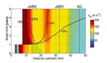
Fig. 11. Time–space distribution of ice surface velocity, u s, in the terminus perturbation simulation (color bar saturates at 200ma–1). Labeled black contours represent the relative magnitude of the velocity perturbation (relative to dynamic equilibrium velocity in year 0) resulting from the catastrophic terminus perturbation event at year 1. Vertical dashed lines denote the locations of JAR2, JAR1 and Swiss Camp (SC). Model time given as relative to the end of spin-up.
5. Summary Remarks
We examined the annual glaciohydrology cycle in the ablation zone of the Sermeq Avannarleq flowline. We coupled a 1-D (depth-integrated) ice-flow model to a previously published 1-D (depth-integrated) hydrology model via a semi-empirical and site-specific basal sliding rule. This sliding rule imposes seasonal perturbations to the background basal sliding velocity that are dependent on rate of change of glacier water storage. Following a 1000year spin-up, the ice-flow model produces dynamic equilibrium ice geometry and velocity fields that compare well with observations. After spin-up, the coupled model reproduces the broad features observed in the annual basal sliding cycle in the terminal 60 km of the flowline, namely: (1) prescribed background basal sliding during the winter;(2) a summer speed-up event;and (3) a fall slowdown event and return to winter velocities. While we have put forth a plausible rule that connects sliding velocity to the state of the glacier hydrologic system, there remains a significant challenge to develop a sliding rule that is more firmly based upon first principles (i.e. no free parameters and based on physical mechanisms by which basal water produces sliding). This requires both a proper characterization of all components of the glacier hydrologic system, from the spatial-temporal pattern of melt generation to the complex evolution of en- and subglacial transport and storage, and a physics-based connection between the state of the hydrologic system and the basal sliding.
GPS observations of ice surface velocity at three stations during 2005 and 2006 suggest the annual velocity cycle propagates as far upstream as ~70km. We examined the relative magnitude of driving and coupling stresses and performed a simple simulation to assess the possible contribution of an upstream propagation of a terminus perturbation through longitudinal coupling to the annual velocity cycle. We find that an extreme terminus perturbation is unlikely to influence velocities upstream of JAR2 (km 14) on the seasonal timescale. Thus, we suggest the annual ice velocity cycle along the majority of the flowline (km 14-70) is instead attributable to the evolution oftheglaciohydrologic system in response to meltwater inputs. Following previous alpine studies, we suggest this local acceleration is due to variations in basal sliding that are governed by variations in the rate of change of glacier water storage, due to local mismatches between surface meltwater input and the ability of the subglacial hydrologic system to transmit water.
Acknowledgements
This work was supported by NASA Cryospheric Science Program grants NNX08AT85G and NNX07AF15G to K.S. and US National Science Foundation (NSF) DDRI 0926911 to W.C. W.C. thanks the Natural Sciences and Engineering Research Council (NSERC) of Canada for support through a Post-Graduate Scholarship, and the Cooperative Institute for Research in Environmental Sciences (CIRES) for support through a Graduate Research Fellowship. R.S.A. acknowledges support through NSF grant EAR 0922126. We thank Gwenn Flowers and an anonymous reviewer for thorough insights on the manuscript. Helen Fricker was our scientific editor.
Appendix: Variable notation

All heads and elevations are in reference to sea level as datum.


