


Introduction
In this paper we investigate the testing of predictive geomechanical models against observations of induced seismicity caused by gas depletion in the Netherlands. In particular, we focus on the onset and growth of seismicity and the reduction of seismicity after a production decrease. The Netherlands qualifies as a suitable case study for such an approach for a number of reasons. In the first place, almost 200 gas fields have been produced to considerable pressure drops in the subsurface. Approximately 15% of these fields have experienced induced seismicity as a result of the gas production. The largest induced earthquake, with a magnitude of M w=3.6 (Fig. 1), occurred in the Groningen field, the largest and most well-documented gas field in the Netherlands, located on the Groningen High. In the second place, the Netherlands is located at a transition from a naturally seismically active area in the south to a naturally seismically quiescent region in the north, which experienced no historic earthquakes prior to gas production. We can therefore be sure that most or all of the earthquakes in the north of the Netherlands are indeed caused by gas depletion. In the third place, key data including the sedimentary structure and fault and fracture fabric are well known from over 30 years of exploration and hydrocarbon production activities, and readily available in public datasets (nlog.nl; Van Wees et al., Reference Van Wees, Buijze, Van Thienen-Visser, Nepveu, Wassing, Orlic and Fokker2014). In recent years, an increasing amount of field data has been collected and studies have been performed on induced seismicity in the Groningen field. A wealth of information on the induced seismicity is given in other papers in this special issue.

Fig. 1. Overview of tectonic elements, seismicity and hydrocarbon reservoirs in the Netherlands. Natural seismicity is shown in red circles, induced seismicity in blue circles (larger events in yellow). Hydrocarbon reservoirs are indicated in green (gas) and red (oil). Major fault zones (solid lines) separate the main tectonic elements which characterize the subsurface of the Netherlands (after Wong et al., Reference Wong, Batjes and de Jager2007). GH/LT = Groningen High/Lauwerszee Trough. Catalogue updated to August 2017. Sources: KNMI (2017) seismic catalogue, NLOG (2012) for depth of top Rotliegend, gas fields and faults. (Modified from Van Wees et al., Reference Van Wees, Buijze, Van Thienen-Visser, Nepveu, Wassing, Orlic and Fokker2014.)
In this paper, we review recent findings from analytical and finite-element-based geomechanical modelling approaches to provide basic understanding of the physical coupling between pressure changes and stress changes in the reservoir, Mohr–Coulomb failure and corresponding seismicity (Fig. 2). In our approach we focus on three key topics, numbered in Figure 2. (1) We outline the main logic of geomechanical modelling approaches and insights developed in recent decades about induced seismicity related to hydrocarbon extraction (Segall, Reference Segall1989; Roest & Kuilman, Reference Roest and Kuilman1994; Segall et al., Reference Segall, Grasso and Mossop1994; Simmelink et al., Reference Simmelink, Orlic and Van Wees2001; Van Wees et al., Reference Van Wees, Orlic, Zijl, Jongerius, Schreppers and Hendriks2001, Reference Van Wees, Buijze, Van Thienen-Visser, Nepveu, Wassing, Orlic and Fokker2014; Van Eijs et al., Reference Van Eijs, Mulders, Nepveu, Kenter and Scheffers2006; Suckale, Reference Suckale2009; Orlic & Wassing, Reference Orlic and Wassing2013; Bourne et al., Reference Bourne, Oates, van Elk and Doornhof2014; Van den Bogert, Reference Van den Bogert2015). Subsequently, as an extension of existing modelling approaches we include (2) rupture models to evaluate the relationship between elastic stress change and seismic moment evolution. Finally, (3) we present the main findings of the approach recently developed by Van Wees et al. (in press) for disentanglement of the effects of pressure change and time-dependent compaction (creep) on the evolution of stress on faults and the subsequent evolution of rupture and seismic moment.
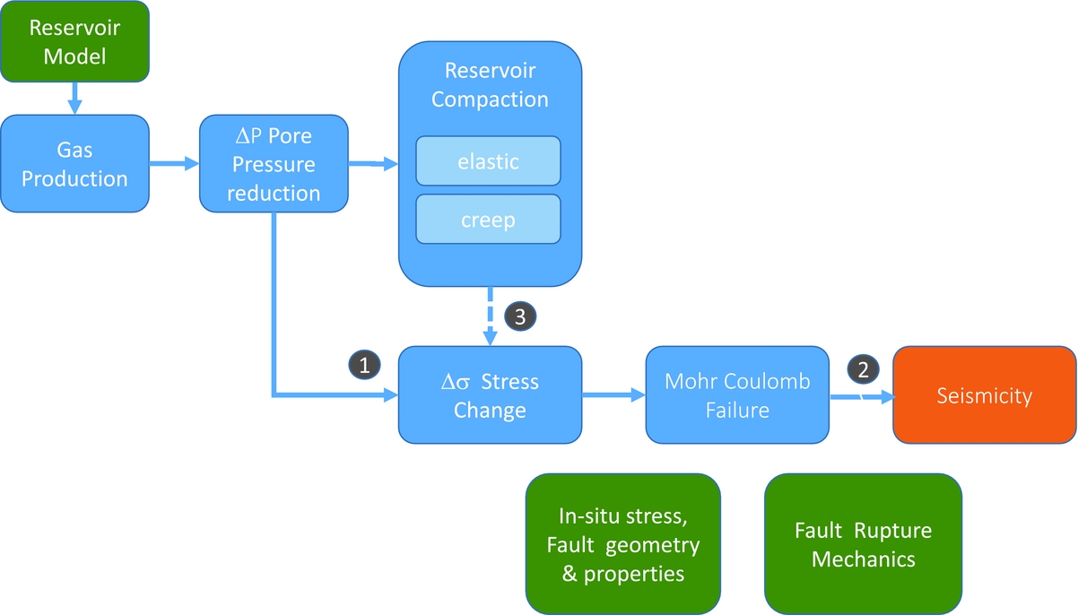
Fig. 2. Geomechanical model approach. Numbers refer to key topics addressed in this paper.
The geomechanical modelling approaches are investigated for a simplified 2D reservoir geometry. The outcomes are compared to field data to investigate generic aspects of the onset of seismicity and growth of seismic moment during production, as well as the evolution of seismic moment in the case of significant reduction or stop of production. To this end we focus on two key observations in the Dutch gas fields, and the Groningen field in particular.
The first observation is that all gas fields in the Netherlands show a delay in the occurrence of induced seismicity, taking at least 28% of relative pressure drop prior to the onset of seismicity as shown in Figure 3 (based on data from (NAM, 2010; Van Thienen-Visser et al., Reference Van Thienen-Visser, Nepveu and Hettelaat2012)). The relationship of relative depletion and observed maximum magnitude is characterised by an upper bound which shows a trend of increasing maximum magnitudes with increasing ΔP/P ini (Van Eijs et al., 2004; Van Thienen-Visser et al., Reference Van Thienen-Visser, Nepveu and Hettelaat2012). Mechanical models predicting moment evolution on faults (e.g. Van Wees et al., Reference Van Wees, Buijze, Van Thienen-Visser, Nepveu, Wassing, Orlic and Fokker2014; Sanz et al., Reference Sanz, Lele, Searles, Hsu, Garzon, Burdette, Kline, Dale and Hector2015) allow us to place the delay of onset and observed increasing growth of seismic moment (Fig. 3; Bourne et al., Reference Bourne, Oates, van Elk and Doornhof2014) in a physical context. Here, we aim to show that mechanical rupture models (Baisch et al., Reference Baisch, Vörös, Rothert, Stang, Jung and Schellschmidt2010) can be used to predict seismic catalogues whose moment evolution appear to be consistent with findings from other mechanical analysis approaches which do not include rupture. We show that mechanical models tend to predict growth of moment strongly bounded by the structural extent of stress perturbations. Consequently, the inferences from the geomechanical models pose a natural limit on predictions of future seismicity, which are low compared to the 10- to 1000-fold increase in cumulative seismic moment inferred by, for example, Bourne et al. (Reference Bourne, Oates, van Elk and Doornhof2014). However, it should be noted that our model has limited quantitative predictive power for the Groningen field, as it is based on a single fault with simplified geometry, and limited parameter variations.

Fig. 3. Local magnitudes of induced events in the Netherlands as a function of depletion pressure. For each field, the depletion parameter (DP/Pini) has been constructed for each earthquake from a linear interpolation of initial pressure to pressures reported at the time of first earthquake (Van Thienen-Visser et al., Reference Van Thienen-Visser, Nepveu and Hettelaat2012) and pressures reported in the NAM report on subsidence evolution (NAM, 2010). Relative pressures for Roswinkel, Groningen, Emmen, Eleveld, Annerveen were calculated from pressure curves shown in Wentinck et al. (Reference Wentinck2016). For the remainder linear extrapolation (modified after Van Wees et al., Reference Van Wees, Buijze, Van Thienen-Visser, Nepveu, Wassing, Orlic and Fokker2014).
Additionally, in view of time-dependent compaction upon reduced production, we focus on the central area of the Groningen field (Fig. 4). In this area, the production rate was decreased by 80%, starting on 17 January 2014 (van Thienen-Visser & Breunese, Reference Van Thienen-Visser and Breunese2015). A statistically significant reduction of seismicity occurred after this production decrease (Nepveu et al., Reference Nepveu, van Thienen-Visser and Sijacic2016). We show that geomechanical models incorporating reservoir creep (Van Wees et al., in press) are in agreement with these observations, independent of the decay rate of time-dependent compaction

Fig. 4. Outline of the Groningen field (red line denotes gas water contact), coloured with pressure change predicted from NAM's reservoir model 1.5 years prior to (left) and after (right) decrease in production 17 January 2014. Induced events until 1 August 2015 for the field are indicated by grey dots (source www.knmi.nl), production clusters by triangles. Induced seismicity of central area within the green polygon is shown in Figure 2, jointly with production data of central area production clusters (orange triangles). The hydraulic diffusivity of the reservoir is such that pressure is equilibrated between production clusters in the central area within months to half a year, whereas pressure diffusion from the edges of the field to the centre would take more than a few years (Van Thienen-Visser & Breunese, Reference Van Thienen-Visser and Breunese2015).
Methods
For Dutch reservoirs, a number of geomechanical numerical modelling studies have studied stress changes and fault reactivation potential associated with gas extraction. Two-dimensional numerical studies have been published on the Eleveld gas field (Roest & Kuilman, Reference Roest and Kuilman1994) and a produced field used for underground gas storage (Nagelhout & Roest, Reference Nagelhout and Roest1997). Mulders (Reference Mulders2003) and Orlic & Wassing (Reference Orlic and Wassing2013) used finite element models to study the stress parameters for a fault-bounded disc-shaped reservoir adopting reservoir geometries representative for Dutch gas depletion, and tested the sensitivity to variability in various rock parameters. Van Wees et al. (Reference Van Wees, Buijze, Van Thienen-Visser, Nepveu, Wassing, Orlic and Fokker2014) investigated the sensitivity of moment evolution as a function of in situ stress. They argue that the faults in the Dutch gas fields are most likely not critically stressed at the onset of depletion as this would have resulted in earlier and stronger seismicity than observed in the Dutch gas fields. Recently, Sanz et al. (Reference Sanz, Lele, Searles, Hsu, Garzon, Burdette, Kline, Dale and Hector2015) and Lele et al. (Reference Lele, Hsu, Garzon, DeDontney, Searles, Gist and Dale2016) presented 3D finite element models of the Groningen field, with similar findings and first-order agreement of predicted and observed cumulative seismic moment in sub-areas of the Groningen Field.
In order to understand the close coupling of predicted moment in geomechanical models with pressure depletion, we introduce the key equations for deriving the moment from predicted displacement. We also use the relation between Coulomb stress change and stress path parameters as a function of pressure depletion, underlying poroelastic parameters, to show the strong influence of fault offset in the stress response. In the subsequent sections the insights from previous studies on the stress path, the incorporation of slip and rupture, time-dependent creep, and choice of the model parameters in simplified models is described.
In a geomechanical model, the expected evolution of cumulative seismic moment (M0) can be determined from predicted slip on faults via (e.g. Van Wees et al., Reference Van Wees, Buijze, Van Thienen-Visser, Nepveu, Wassing, Orlic and Fokker2014):
 $$\begin{equation}
M0 = \smallint G\ u\ dS\
\end{equation}$$
$$\begin{equation}
M0 = \smallint G\ u\ dS\
\end{equation}$$
where S is surface area of faults, u is relative displacement and G is the shear modulus of the host rock. The onset and subsequent amount of slip is a function of the change in Coulomb failure function (ΔCFF) in relation to the in situ stress:
 $$\begin{equation}
\Delta {\rm{CFF}} = \Delta \tau - \ \mu \Delta {\sigma _{\rm{n}}}^{\prime}
\end{equation}$$
$$\begin{equation}
\Delta {\rm{CFF}} = \Delta \tau - \ \mu \Delta {\sigma _{\rm{n}}}^{\prime}
\end{equation}$$
where τ is the shear stress on the fault, σn′ is the effective normal stress on the fault, and μ is the fault's friction coefficient. Compressive stresses are denoted positive. In elastic models, ΔCFF scales linearly to pressure change ΔP through changes in the total stress tensor on the fault (Mulders, Reference Mulders2003; Soltanzadeh & Hawkes, Reference Soltanzadeh and Hawkes2008):
 $$\begin{equation}
\Delta \sigma _{ij}^{\prime} = \alpha ({\gamma _{ij}} - {\delta _{ij}})\ \Delta P
\end{equation}$$
$$\begin{equation}
\Delta \sigma _{ij}^{\prime} = \alpha ({\gamma _{ij}} - {\delta _{ij}})\ \Delta P
\end{equation}$$
where σ
ij
are the total stress tensor components, and γ
ij
normalised stress path parameters, describing the stress path in terms of change in stress tensor as a function of pressure change. α corresponds to Biot's coefficient, which is generally set to 1 (Mulders, Reference Mulders2003; Van Wees et al., Reference Van Wees, Buijze, Van Thienen-Visser, Nepveu, Wassing, Orlic and Fokker2014). δ
ij
are tensor components of the Identity matrix. Gas depletion results in a negative ΔP. Equation 3 applies to the parts of the fault subject to the reservoir pressure, whereas δ
ij
= 0 holds for the parts of the fault which are not subject to the reservoir pressure. The stress path parameters are a function of poroelastic parameters, fault geometry and offset (Fig. 5), and can be determined semi-analytically from linear poroelasticity, or numerically (Mulders, Reference Mulders2003; Soltanzadeh & Hawkes, Reference Soltanzadeh and Hawkes2008). For laterally extensive reservoirs
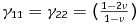 ${\rm{\ }}{\gamma _{11}} = {\gamma _{22}} = ( {\frac{{1 - 2\nu }}{{1 - \nu }}} )$
in agreement with uniaxial compaction. The other components of γ
ij
are 0, resulting in an increase of horizontal stress with pressure depletion. For reservoirs bounded by faults or internally faulted reservoirs with offset along the faults, the stress path parameters vary over the fault surface, but behave stationarily through time under spatially uniform depletion. The associated stress paths are well capable of predicting an accelerating increase of seismic moment as a function of pressure change assuming elastic deformation (Van Wees et al., Reference Van Wees, Buijze, Van Thienen-Visser, Nepveu, Wassing, Orlic and Fokker2014). Mulders (Reference Mulders2003) and Van Wees et al. (Reference Van Wees, Buijze, Van Thienen-Visser, Nepveu, Wassing, Orlic and Fokker2014) highlight that ΔCFF for laterally extensive reservoirs strongly depends on ν, and effects of differential compaction on ΔCFF are far more pronounced on faults bounding or offsetting the reservoirs (Fig. 6). In the Groningen field the pressure change is spatially rather uniform, and the pressure is linearly decreasing in the last 30 years (Bourne et al., Reference Bourne, Oates, van Elk and Doornhof2014; Van Wees et al., Reference Van Wees, Buijze, Van Thienen-Visser, Nepveu, Wassing, Orlic and Fokker2014).
${\rm{\ }}{\gamma _{11}} = {\gamma _{22}} = ( {\frac{{1 - 2\nu }}{{1 - \nu }}} )$
in agreement with uniaxial compaction. The other components of γ
ij
are 0, resulting in an increase of horizontal stress with pressure depletion. For reservoirs bounded by faults or internally faulted reservoirs with offset along the faults, the stress path parameters vary over the fault surface, but behave stationarily through time under spatially uniform depletion. The associated stress paths are well capable of predicting an accelerating increase of seismic moment as a function of pressure change assuming elastic deformation (Van Wees et al., Reference Van Wees, Buijze, Van Thienen-Visser, Nepveu, Wassing, Orlic and Fokker2014). Mulders (Reference Mulders2003) and Van Wees et al. (Reference Van Wees, Buijze, Van Thienen-Visser, Nepveu, Wassing, Orlic and Fokker2014) highlight that ΔCFF for laterally extensive reservoirs strongly depends on ν, and effects of differential compaction on ΔCFF are far more pronounced on faults bounding or offsetting the reservoirs (Fig. 6). In the Groningen field the pressure change is spatially rather uniform, and the pressure is linearly decreasing in the last 30 years (Bourne et al., Reference Bourne, Oates, van Elk and Doornhof2014; Van Wees et al., Reference Van Wees, Buijze, Van Thienen-Visser, Nepveu, Wassing, Orlic and Fokker2014).

Fig. 5. Geometry set-up for the simplified 2D geomechanical model. The offset of the fault is indicated relative to the thickness of the reservoir D.
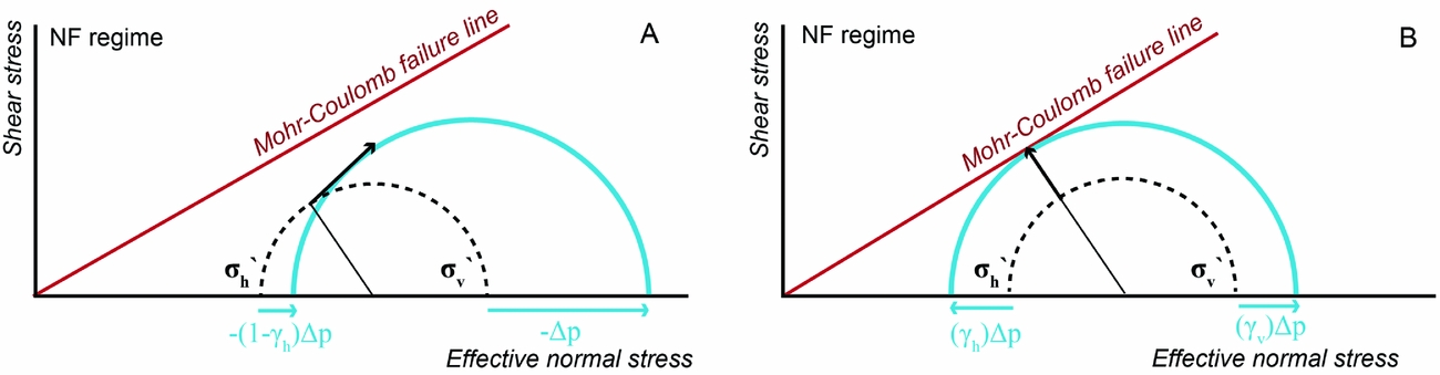
Fig. 6. Schematic Mohr circles corresponding to stress path parameters γ11 = γh and γ33 = γv of horizontal and vertical stress respectively along a horizontal mid-line of a laterally extensive reservoir (A) and a side bounded reservoir with rectangular geometry under plane strain conditions (B). Biot's coefficient α=1 (after Van Wees et al., Reference Van Wees, Buijze, Van Thienen-Visser, Nepveu, Wassing, Orlic and Fokker2014).
Insights from previous studies
From analytical and numerical finite element studies the following generic characteristics have been observed:
-
• Representative geometries for Dutch gas fields are marked by typical thickness to half-length ratios of about 0.1, and depth to thickness ratios exceeding 10 (Mulders, Reference Mulders2003; Orlic & Wassing, Reference Orlic and Wassing2013; Van Wees et al., Reference Van Wees, Buijze, Van Thienen-Visser, Nepveu, Wassing, Orlic and Fokker2014). The magnitude of the stress path parameters for differential compaction is hardly changing at the side bounding faults/edge, if these ratios are changed (Soltanzadeh & Hawkes, Reference Soltanzadeh and Hawkes2008).
-
• The accentuated stress path parameters of differential compaction at a fault (Fig. 6) typically decline rapidly over a relatively short distance of about half the thickness of the reservoir away from the fault to values in agreement with the uniaxial compaction for laterally extensive reservoirs. This is supported by findings from both 2D and 3D geomechanical models (e.g. Orlic & Wassing, Reference Orlic and Wassing2013; Lele et al., Reference Lele, Garzon, Hsu, DeDontney, Searles and Sanz2015; Van den Bogert, Reference Van den Bogert2015).
-
• The accentuated stress path parameters caused by differential compaction at faults is also in agreement with a recent update of predictive seismological models for the Groningen field based on volumetric and fault-related shear strains of the reservoir (Bourne & Oates, Reference Bourne and Oates2015). This study outlines sourcing of predicted seismic event rates at faults offsetting the reservoir. It is also supported by localisation of seismic events on faults in the reservoir by full waveform inversion of data collected in deep monitoring wells (NAM, 2016).
-
• The characteristics of γ ij at the horizontal mid-line of the reservoir are not sensitive to changing vertical faults to more realistic steeply dipping faults at the side boundary (e.g. Mulders, Reference Mulders2003).
-
• The thickness of the reservoir at the side boundary plays an important factor in the areal extent which is marked by exceedance of critical stress (e.g. Orlic & Wassing, Reference Orlic and Wassing2013). Since the seismic moment of an event is proportional to the slipping area of the fault, the thickness is expected to play an important role in the level of seismicity which can be generated, through an increase of the area of seismic slip and the associated displacement. Stress effects can be amplified for offsetting reservoirs compared to side bounded reservoirs, depending on the pressure condition in the fault (e.g. Orlic & Wassing, Reference Orlic and Wassing2013)
-
• A contrast in the ratio of Young's moduli of overburden and reservoir has a significant effect on the maximum values of γ ij which are attained. Mulders (Reference Mulders2003), Van Eijs et al. (Reference Van Eijs, Mulders, Nepveu, Kenter and Scheffers2006) and Van den Bogert (Reference Van den Bogert2015) demonstrate that ΔCFF becomes amplified with increasing contrast in elastic properties of reservoir and surrounding rock.
-
• Creep effects in evaporite cap rocks can result in time-dependent effects in strain and stress reponse (e.g. Orlic & Wassing, Reference Orlic and Wassing2013).
-
• Biot's coefficient scales the stress response. Recent laboratory measurements on Groningen field rocks indicate a range of 0.6–1, as a function of porosity (Lele et al., Reference Lele, Garzon, Hsu, DeDontney, Searles and Sanz2015). This implies that low-porosity areas of the reservoir experienced 60% of the maximum stress response expected compared to most porous areas.
The aforementioned studies have successfully addressed the phenomenological explanation for various features of induced seismicity observed in Dutch gas fields. For predictive purposes, the two-dimensional approaches fail to capture the effects of full structural complexity, whereas the numerically intensive three-dimensional models have major difficulty in incorporating sufficient resolution and uncertainty for data assimilation and probabilistic predictions. As mentioned before, in this paper we focus on two generic and phenomenological aspects, which have received little attention: the effects of adopting rupture models and time-dependent compaction.
Fault slip and rupture
Various algorithms exist to determine the area of slip and displacement of a fault surface when ΔCFF exceeds the yield surface. Finite-element models provide techniques to evaluate the plastic slip based on a minimum work approach but are computationally intensive as they require many iterations, especially for 3D models (e.g. Orlic & Wassing, Reference Orlic and Wassing2013; Sanz et al., Reference Sanz, Lele, Searles, Hsu, Garzon, Burdette, Kline, Dale and Hector2015). Semi-analytical approaches such as proposed by Madariaga (Reference Madariaga1979) and Van Wees et al. (in press) allow us to approximate the seismic moment density of a normal fault from the elastic stress solution. In an elastic solution ΔCFF results in an average excess Coulomb stress Δσ relative to the Mohr–Coulomb failure criterion over the rupture length l. The seismic moment density M0m (unit N) of the fault per unit length in strike becomes:
 $$\begin{equation}
M{0_{\rm{m}}} = \Delta \sigma \frac{{\ {l^{2}}}}{{\sqrt \pi }}
\end{equation}$$
$$\begin{equation}
M{0_{\rm{m}}} = \Delta \sigma \frac{{\ {l^{2}}}}{{\sqrt \pi }}
\end{equation}$$
Equations 3 and 4 clearly demonstrate the linear relationship between moment density increase and pore pressure change on a fault, provided the dip-slip rupture length l and strike dimensions of the slipping faults do not change. However, both are bound to change over time: l grows with increasing stress change, and the strike dimension of faults is bound to grow with progressively more fault orientations becoming critically stressed, depending on the in situ stress (Fig. 4).
Equation 4 assumes that all moment is directly released seismically and is not marked by energy losses or changing frictional properties upon slip. From laboratory experiments it is well known that the friction angle of the slipping portion of the fault is reduced upon slip initiation, resulting in more slip until a new balance is found for the stabilised stresses after slip and the reduced friction angle (e.g. Niemeijer & Spiers, Reference Niemeijer and Spiers2007). Numerical inclusion of slip-weakening effects and/or rate and state friction effects during rupture events result in a less smooth build-up of seismic moment and can produce synthetic seismic catalogues with characteristics similar to actual catalogues (Baisch et al., Reference Baisch, Vörös, Rothert, Stang, Jung and Schellschmidt2010; Rutqvist et al., Reference Rutqvist, Rinaldi, Cappa and Moridis2013; Wassing et al., Reference Wassing, Van Wees and Fokker2014).
We calculate the co-seismic change of the shear stress, using a slider-block model with static and dynamic coefficients of friction, μs and μd (Zielke & Arrowsmith, Reference Zielke and Arrowsmith2008), which, for simplicity, changes instantaneously upon slip initiation. It therefore represents a perfect seismogenic material, in which all slip is converted into seismic energy. In more sophisticated rate-and-state models, the friction angle drop is dependent on slip velocity and is therefore generally marked by aseismic slip if velocities are low (Richards-Dinger & Dieterich, Reference Richards-Dinger and Dieterich2012). In our model, the fault is discretised in small patches. The co-seismic phase starts with a seismic activity when at least one fault patch becomes activated through stresses exceeding the Mohr–Coulomb criterion with the static friction coefficient μs. The friction coefficient of activated patches then changes instantaneously to its dynamic value, μs➔μd. For seismic fault patches, the dynamic friction coefficient is smaller than the static one, resulting in a release of stress so that the new shear stress is τ = μdσ′n. The model ignores potential inertia effects, which can result in an overshoot of release of stress. A seismic event may grow because slip along one patch induces stress changes along the other patches. We assume no energy is lost or gained in the stress transfer. If these changes are sufficient to cause other patches to fail, they will do so as part of the same seismic event. The friction coefficient of activated patches remains at the dynamic level for the duration of the event. Patches may slip more than once and continue to do so as long as τ = μdσ′n. The event is over when τ along all fault patches is at or below a level corresponding to the dynamic friction coefficient μd. In the model, the seismic moment is calculated from the integral of slip of the ruptured patches times the rupture area times shear modulus G (Equation 1). Then the next interseismic phase is entered, all patches instantaneously regain their static coefficient assuming healing and the loading mechanism resumes. The loading for the rupture model comes from the stress changes which are calculated by a finite element model (not incorporating slip), at many regular intervals (e.g. Wassing et al., Reference Wassing, Van Wees and Fokker2014).
To calculate the stress transfer from a failing patch to all other patches we use Okada's kernel of boundary element method (Okada, Reference Okada1992). Okada's solutions represent a complete set of closed analytical expressions in a unified manner for the internal displacements and strains due to shear and tensile faults in a half-space for both point sources and for finite rectangular sources. In alternative models such as proposed by Baisch et al. (Reference Baisch, Vörös, Rothert, Stang, Jung and Schellschmidt2010) it is assumed that only 90% of the stress is transferred from one patch to the other for patch sizes of 20m. This effectively results in a seismic moment which is c. 10% of the seismic moment predicted from a 100% stress transfer as adopted in this paper. On the other hand, inertia effects can amplify near-field stress transfer and increase the released seismic moment (e.g. Buijze et al., Reference Buijze, Van den Bogert, Wassing, Orlic and ten Veen2017).
The rupture models are particularly useful to understand the process of transfer of Coulomb stress to seismic moment as a function of stress drop, in situ stress, cohesion, fault roughness etc. As they generate catalogues of seismicity, the results can be directly compared to observations such as Gutenberg–Richter characteristics. Rupture models need to account for natural roughness of the fault surface (or underlying frictional properties or cohesion) in order to avoid cycles of simultaneous rupture patches (e.g. Baisch et al., Reference Baisch, Vörös, Rothert, Stang, Jung and Schellschmidt2010). For the roughness of faults, we adopt the algorithm as proposed in Dieterich & Richards-Dinger (Reference Dieterich and Richards-Dinger2010), with physical distortion of the fault surface in the normal direction, following a spatially correlated normal function. The relative roughness is characterised by the parameter β, which is varied from 0 (no roughness) to values of about 0.03 (maximum roughness) in this study.
Model geometry and parameterisation
The stress changes related to reservoir depletion have been calculated from a 2D plane-strain finite element model of a depleting gas reservoir. The model geometry, in terms of depth and thickness range, and the underlying parameterisation are inspired by 2D models for the Groningen gas field (e.g. Van den Bogert, Reference Van den Bogert2015). For the finite element modelling we use DIANA FEA (http://dianafea.com). More details of the finite element modelling procedure are given in Orlic & Wassing (Reference Orlic and Wassing2013) and the online manual of DIANA FEA.
The numerical model incorporates two reservoir compartments, separated by a fault with a throw of half the reservoir thickness (Fig. 5; Table 1), which can be considered representative for major fault zones in the central area of the Groningen field, in the vicinity of which most seismic events have occurred (Fig. 4; Bourne et al., Reference Bourne, Oates, van Elk and Doornhof2014). The plane-strain finite element mesh models a 2D section 6km wide and 6km deep. The model consists of roughly 135,000 nodes which comprise c. 44,000 quadratic quadrilateral plane-strain elements representing the bulk rock and ~250 quadratic interface elements representing the fault. The model is laterally constrained (zero horizontal displacement) on the sides and vertically constrained (zero vertical displacement) at the bottom, and subject to gravity loading. This effectively leads to a stress response on the sides of the model which corresponds to an infinite lateral extension of the reservoir.
Table 1. Parameters of the geomechanical model.

For rupture modelling we extend the reservoir geometry in 3D assuming a reservoir side length of 3500m (Van Wees et al., Reference Van Wees, Buijze, Van Thienen-Visser, Nepveu, Wassing, Orlic and Fokker2014), taking the elastic stress response from the 2D model as input. The rupture surface measures 4km in strike and 2km in dip direction of the fault. We subdivide the fault in patches of 50×50m and apply the rupture model with a constant friction angle drop of 3°, with static friction angle of 30°. The fault surface is marked by a slight natural geometrical roughness (β=0.01, Dieterich & Richards-Dinger, Reference Dieterich and Richards-Dinger2010), preventing large portions of the fault from being critically stressed at exactly the same time. The stress loading of reservoir depletion is applied in 1000 load steps.
The initial pressure is characterised by overpressures, through a hydrostatic gradient with abnormally high fluid density of 1150kgm−3, resulting in c. 35MPa at reservoir depth in agreement with initial pressures observed in the Groningen field (Bourne et al., Reference Bourne, Oates, van Elk and Doornhof2014). The initial ratio of effective horizontal-to-vertical stress is set to K0eff=0.45. The final depletion in the reservoir is 25MPa, approximately in agreement with present-day pressure depletion in the field. Depletion is implemented to occur simultaneously, at the same rate, in both reservoir compartments in yearly load steps. The pressure depletion of 25MPa is built up linearly in a time period of 60 years, representing the time period prior to decrease in production on 17 January 2014. The reduction in pore pressure is the same for all values of the horizontal coordinate, in agreement with high diffusion rates observed in the Groningen gas field, marked by a delay time of a couple of months to equilibrate pressures from the well cluster in the central area (Van Thienen-Visser & Breunese, Reference Van Thienen-Visser and Breunese2015). The linear pressure depletion rate has been constrained by the observed linear pressure reduction in the last 30 years prior to the recent decrease in production (Bourne et al., Reference Bourne, Oates, van Elk and Doornhof2014). The time period of pressure depletion has been extended to 60 years relative to the ~50 years of actual production in the field, to compensate for higher pressure rate changes in the first 20 years of production (e.g. Mossop, Reference Mossop2012; Bourne et al., Reference Bourne, Oates, van Elk and Doornhof2014).
For the models studying the onset and growth of seismicity up to the moment of decrease in production, we discard time-dependent creep effects and adopt the parameters listed in Table 1. In addition, we use the elasto-plastic capability for Mohr–Coulomb failure and slip of the finite element code for comparing slip and moment from the 2D plane strain model with the results of the 3D rupture model.
The fault zone in the 2D and 3D approaches is assumed to be subject to the reservoir fluid pressure when reservoir rock is present on both sides of the fault. For the portion of the fault where reservoir rock and surrounding rock are juxtaposed, we considered two scenarios for pressure in the fault: following the reservoir pressure or ambient (initial reservoir) pressure.
Obviously, a single fault geometry cannot capture the complex response expected from many mapped faults in the area with variable throw, dip and strike (Fig. 3). Uncertainty in the location of seismic events hampers an allocation of seismic events to particular faults. It is clear that fault strike, dip, throw, natural stress variability, and variability in mechanical properties, all have a significant control on in situ stress and spatial and temporal variability in seismicity. However, these effects are not expected to have a prime control on the relative change in seismic response upon production changes, as these do not strongly affect the ΔCFF for a given pressure change.
The cap rock of the reservoir of the Groningen field consists of evaporites, which are likely not able to support significant shear stress and will therefore likely not experience seismic slip. This is currently neglected in the model, and the results therefore overestimate l and the associated moment. In view of Equation 4, this may amount to factor of 4, if l would be reduced by a factor of 2.
Onset and growth of induced seismicity
The elastic stress response of the finite element model due to depletion is shown in Figures 7 and 8. At 25MPa of pressure depletion, a portion of the fault exceeds the Mohr–Coulomb criterion and slip would initiate at c. 30% (7.5MPa depletion) and 60% (15MPa depletion) of the final depletion for the reservoir and ambient pressure scenarios. Figure 9 shows the results from incorporating plastic failure in the finite element model. The moment evolution is marked by a short initial stage of increasing growth, related to growth of l, followed by more linear growth with time as l becomes stationary (see Equation 4). This is in agreement with the linear behaviour of stress change through time.

Fig. 7. Finite element model solutions for gas depletion with 0.5D offset. (A) Pore pressure on the fault assuming reservoir pore pressure, (B) pore pressure on the fault assuming ambient pore pressure, (C) effective normal stress on the fault assuming reservoir pore pressure, (D) effective normal stress on the fault assuming ambient pore pressure, and (E) shear stress on the fault, identical for both pore pressure assumptions. The sign of shear stress is positive if shear sense is normal faulting. The depth extent of the reservoir zones is indicated on both sides of the fault in grey.
Fig. 8. Finite element model solutions for change in Coulomb failure function on the fault (cf. Fig. 7) assuming (A) reservoir and (B) ambient pore pressure. The grey line corresponds to the failure criterion.
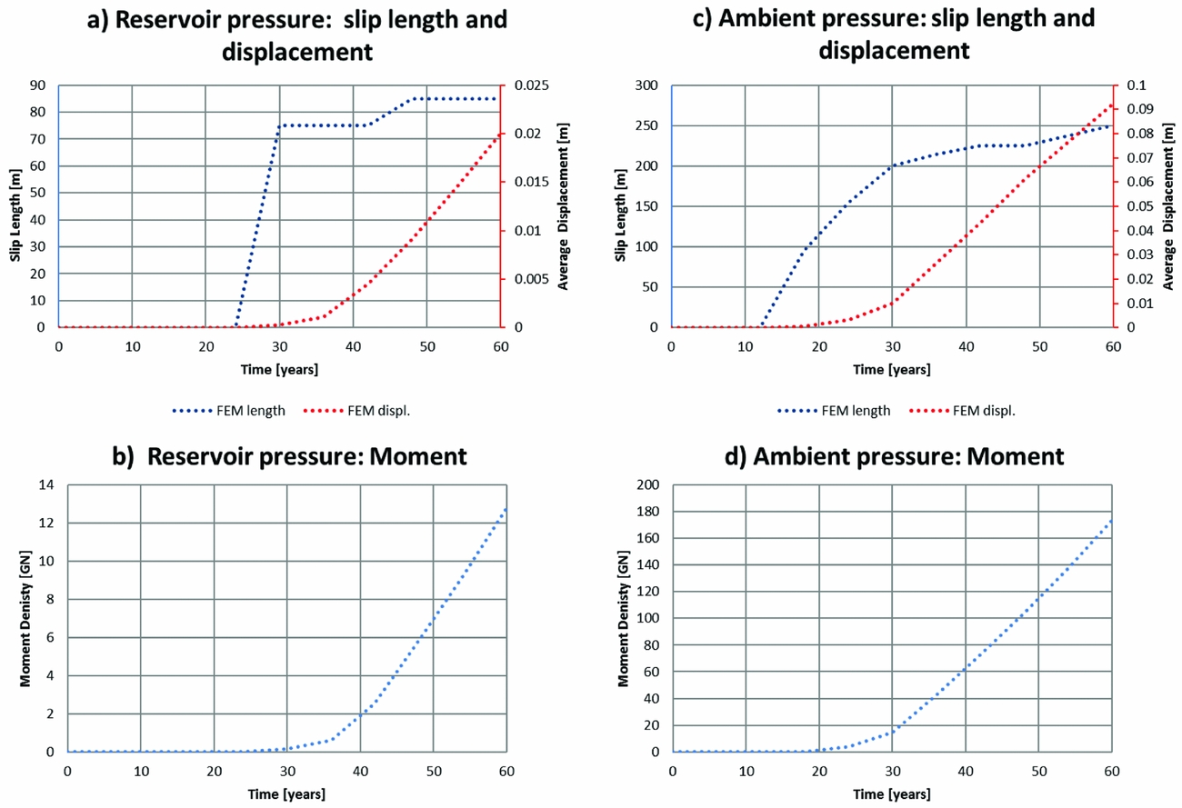
Fig. 9. Comparison of slip length, displacement and moment predicted by finite element analyses incorporating Mohr–Coulomb failure and slip.
Figures 10 and 11 show the results for subcritical in situ stress conditions in agreement with K0eff=0.45 for reservoir and ambient pressure conditions in the fault zone (Fig. 8a and b respectively). Figures 12 and 13 show model runs for critical in situ stress conditions in agreement with K0eff=0.4 for reservoir and ambient pressure conditions. Figure 14 compares the moment evolution for the model runs – referred to as base case – to alternative models. One of the alternative models is a run with a negligible friction angle drop of 0.1°, showing a close resemblance to the moments predicted by the finite element model (both in timing and magnitude), in Figure 9. The latter need to be multiplied by 3500m (the reservoir side length in the rupture models) to compare them to moments in Figure 14.

Fig. 10. Rupture model results for finite element stresses for 0.5D model with reservoir pressure. Stress is incremented in 1000 load steps. Left: dip-slip displacement; middle: Coulomb stress relative to Mohr–Coulomb failure (numbers are negative below failure); right: Gutenberg–Richter plot of resulting earthquake catalogue. Non-critical stress is assumed initially (K0eff=0.45).

Fig. 11. Rupture model results of 25MPa pressure depletion for finite element stresses for 0.5D model with ambient pressure, with non-critical in situ stress (K0eff=0.45).

Fig. 12. Rupture model results of 25MPa pressure depletion for finite element stresses for 0.5D model with reservoir pressure, with close to critical in situ stress (K0eff=0.4).

Fig. 13. Rupture model results of 25MPa pressure depletion for finite element stresses for 0.5D model with ambient pressure, with close to critical in situ stress (K0eff=0.4).

Fig. 14. Evolution of the cumulative seismic moment from the rupture models. The base case scenarios and critically stressed scenarios are according to K0eff=0.45 (Figs 10 and 11) and K0eff=0.4 (Figs 12 and 13) scenarios respectively. The cohesion scenario is marked by 3MPa cohesion relative to the base case. For reservoir pressure the cohesion scenario does not reach failure. The azimuth 60 scenario is marked by in situ stress conditions with minimum horizontal stress orientated at 60° from the strike of the fault, instead of 90° in the base case. The stress drop 0.1 scenario is marked by a friction angle drop of 0.1°, resembling the moment evolution depicted in Figure 9.
The rupture process can be considered as a domino effect in which the height of the dominos is given by reduction of friction angle through slip (also called stress drop), and the spacing between the dominos by the stability of the in situ stress (how far it is from failure). If faults are already critically stressed at the start of production, the dominos are close to each other, and create large rupture surfaces early in the depletion history. When the faults are not critically stressed initially, the dominos are further apart and will only result in larger rupture areas after some period of depletion. Rupture surfaces tend to be restricted to the part of the fault area where compaction-induced stresses build up.
The simple model highlights the strong sensitivity of the occurrence of events as a function of in situ stress on faults. In the case of a critically stressed fault (Figs 12 and 13), events occur almost immediately after onset of production and their magnitudes are more-or-less the same over the whole time interval. The highest magnitude corresponds to rupture extending to significant portions of the fault outside the reservoir level, clearly visible in Figure 13. Remarkably, when assuming reservoir pressures in the fault, the rupture surface is not capable of growing outside the reservoir level, strongly limiting the reservoir seismicity compared to the ambient pressure scenario. This contrast is related to the rims of strongly negative ΔCFF in the reservoir pressure scenario preventing stress transfer from resulting in avalanching of rupture over these rims.
In the case of a non-critically stressed fault, events only occur after some time and there is a build-up in the magnitude of the events that take place. The evolution of the Gutenberg–Richter characteristics for both the reservoir and the ambient pressure scenario shows an increase of the Gutenberg–Richter maximum magnitude with increasing depletion. The associated exponential increase in seismic moment appears more in line with observations than the critically stressed scenario. The long delay in onset of seismicity corresponds well to the Groningen field where seismicity was first registered in December 1991 while production was started in 1964. Additionally, a build-up of seismic events is also observed in Groningen (increasing event rates and increasing magnitudes). Even though this model only shows a single fault, the characteristics of the occurrence of the seismic events in Groningen are present.
The Gutenberg–Richter relationship of the different model runs is given in Figure 15 further below. In the Groningen field b-values are close to 1 (e.g. Van Wees et al., Reference Van Wees, Buijze, Van Thienen-Visser, Nepveu, Wassing, Orlic and Fokker2014). The modelled b-values are close to 1 throughout the depletion history for critically stressed scenarios (Figs 12 and 13), whereas for the subcritical in situ stress the b-values are close to 1 in the lower-magnitude range but the Gutenberg–Richter relationship appears truncated by a lower magnitude than the critically stressed scenarios. This is most likely related to the spatial confinement of the predicted events to the reservoir level in combination with the simplified geometry of the fault model.

Fig. 15. Gutenberg–Richter plots for seismic catalogues predicted by the rupture models. Scenarios as in Figure 14.
We performed various sensitivity runs of the rupture model. These are shown in Figures 14 and 15. The base case scenarios and critically stressed scenarios are according to K0eff=0.45 (Figs 10 and 11) and K0eff=0.4 (Figs 12 and 13) scenarios respectively. The scenario with fault cohesion is marked by 3MPa cohesion, whereas the base case does not include fault cohesion. The cohesion scenario with reservoir pressure on the fault is absent in the plot as it does not reach failure under the imposed loading conditions. The azimuth 60 scenario is marked by in situ stress conditions with minimum horizontal stress orientated at 60° from the strike of the fault, instead of 90° in the base case. The stress drop 0.1 scenario is marked by a friction angle drop of 0.1°, resembling the moment evolution depicted in Figure 9. Comparison of the moment evolution of the negligible stress drop scenario with other scenarios shows that increased stress drop causes the moment evolution to be rougher (as expected because of the increased moment release by individual seismic events) and markedly more upward concave. The strong sensitivity of timing and final total seismic moment to cohesion and relative orientation of the fault in the stress field shows that variability in these parameters can strongly control the spatial and temporal distribution of the cumulative moment of multiple faults. However, it should be noted that if deviation from optimal orientation would be too large, new faults could be formed.
The model results confirm the findings of Van Wees et al. (Reference Van Wees, Buijze, Van Thienen-Visser, Nepveu, Wassing, Orlic and Fokker2014) that a subcritical stress state is consistent with the observed late onset of seismicity and nonlinear growth of seismicity in the field.
The current accumulated total seismic moment in the Groningen field amounts to c. 1015Nm (e.g. Bourne et al., Reference Bourne, Oates, van Elk and Doornhof2014). The predicted moment in the models is order 1014Nm and 1015Nm for the base case reservoir and ambient pressure models respectively. In the geomechanical models, 4–40km of fault length would suffice to generate the observed cumulative moment. This is about one order lower than expected from the distribution of seismicity and faults in the field (Fig. 4). A factor 4 of this mismatch can be explained by the fact that evaporitic cap rock will absorb a significant portion of the seismic moment as explained in the previous section. Additionally, a Biot's coefficient lower than 1 has a significant effect on lowering stress change with pressure change. Furthermore, up to a factor of 10 of seismic moment may be absorbed by aseismic slip as suggested by applications of rupture models in other settings (e.g. Baisch et al., Reference Baisch, Vörös, Rothert, Stang, Jung and Schellschmidt2010; Wassing et al., Reference Wassing, Van Wees and Fokker2014).
The cumulative moment of all rupture models is marked by a concave pattern when plotted on logarithmic scale (Fig. 14) and seems to underestimate the observed increasing growth marked by more-or-less linear growth of log moment as a function of pressure depletion (Fig. 3) and compaction (cf. the partition coefficient in Bourne et al., Reference Bourne, Oates, van Elk and Doornhof2014). Various mechanisms can be considered which can explain this discrepancy, including:
-
• Cumulative effect of multiple faults with different orientation: the model considers a single fault. However, the Groningen field consists of multiple faults with different orientation in the stress field (Fig. 4). The progressive contribution of an increased number of faults will contribute to the enhancement of nonlinear growth.
-
• Evolutionary effects of slip to seismic transfer: it is likely that a fraction of the slip is seismic, and more sophisticated rupture models (e.g. Buijze et al., Reference Buijze, Van den Bogert, Wassing, Orlic and ten Veen2017) show that the ratio of seismic and aseismic slip is likely to increase as a function of rupture length.
-
• Rate-dependent effects: a transition from reservoir pressure support tow ambient pressure support could occur at relatively fast depletion rates, in the last 10 years of production.
-
• Matrix: faults which have not been mapped and are marked with negligible offset compared to thickness can become progressively critically stressed through the stress path for a laterally extensive reservoir (Fig. 5a). The stress path is dependent on Biot's coefficient and ν, which in turn may be strongly dependent on porosity (e.g. Lele et al., Reference Lele, Hsu, Garzon, DeDontney, Searles, Gist and Dale2016).
In addition, it should be stressed that the 2D model is far too simplified to capture the effects of spatial variability in fault strike, dip, reservoir offset and thickness, initial stress, etc.
Summarising, the numerical models indicate that the initial stress ratio in the Groningen field and the Dutch subsurface in general is most likely not close to the critical stress values for failure of existing faults. A critical stress state would trigger earthquakes from the start of gas production if faults are close to optimally oriented. The log moment is marked by a concave-upward growth of seismicity in time. This concave pattern is also predicted by 3D finite element studies of the Groningen field (Sanz et al., Reference Sanz, Lele, Searles, Hsu, Garzon, Burdette, Kline, Dale and Hector2015; Lele et al., Reference Lele, Hsu, Garzon, DeDontney, Searles, Gist and Dale2016). For future prediction, such upward-concave patterns strongly suggest, from a mechanical point of view, that seismic moment is highly unlikely to grow to 100 times higher values in the future, in the range of 1017Nm, as inferred by Bourne et al. (Reference Bourne, Oates, van Elk and Doornhof2014). However, this inference needs to be interpreted with care as the geomechanical models are simplified and do not take into account (spatial) uncertainty of underlying parameterisation.
The presented model serves to highlight key aspects of the interaction of initial stress and differential compaction in the framework of induced seismicity in Dutch gas fields. It is not intended as a predictive model for induced seismicity in a particular field. To this end, a much more detailed field-specific study, taking into account the full complexity of reservoir geometry, depletion history, mechanical properties and underlying uncertainty, is required.
Reduction of seismicity after production stop: the mechanical effects of creep
For a geomechanical model that does not incorporate reservoir creep (Fig. 8), the normalised stress changes and increase in seismic moment would completely arrest when production and associated pressure changes in the field stop. In this section, we address the stress evolution and seismic moment evolution during production and up to 40 years after a production stop, incorporating Kelvin-chain creep for reservoir creep (Table 2). This scenario incorporates a ratio of 1 for final reservoir creep compared to final elastic compaction. More details on the modelling procedure, results and underlying sensitivities can be found in Van Wees et al. (in press). Here we highlight the main outcomes of the modelling study.
Table 2. Viscoelastic parameters in the Kelvin-chain model (Fig. 7). Viscosity η1 is chosen such that it agrees with a relaxation time λ1=7.3 years (Mossop, Reference Mossop2012).

The details of incorporating time-dependent creep through a Kelvin-chain constitutive model are extensively described in Van Wees et al. (in press), and briefly outlined here. The Kelvin-chain model is a seasoned creep model in finite element approaches. For uniaxial strain, the Kelvin-chain model corresponds to the decay model proposed by Mossop (Reference Mossop2012) for time-dependent reservoir compaction. The Kelvin-chain model is marked by an exponential decay, predicting large time-dependent strain in the first years after a sudden halt in pressure change compared to rate type and linear compaction models (e.g. Pruiksma et al., Reference Pruiksma, Breunese, van Thienen-Visser and de Waal2015), for the same amount of final time-dependent compaction. In this sense, the Kelvin-chain model can be considered most pessimistic in terms of reservoir strains and stress changes associated with these strains.
The Kelvin chain contains an elastic component with spring constant E and dashpot with spring constant E 1 and Newtonian viscosity η 1 representing the time-dependent compaction (Fig. 16). The creep component of the uniaxial compaction strain is constructed by the convolution (Mossop, Reference Mossop2012; Van Wees et al., 2017):
 $$\begin{equation}
{\varepsilon _{cz}}\left( t \right) = f'*g
\end{equation}$$
$$\begin{equation}
{\varepsilon _{cz}}\left( t \right) = f'*g
\end{equation}$$
with
 $$\begin{equation*}
f\left( t \right) = \frac{1}{{{\lambda _1}}}{e^{ - t/{\lambda _1}}}\
\end{equation*}$$
$$\begin{equation*}
f\left( t \right) = \frac{1}{{{\lambda _1}}}{e^{ - t/{\lambda _1}}}\
\end{equation*}$$
 $$\begin{equation*}
g\left( t \right) = {C_{{\rm{tinf}}}}\ {\rm{\Delta }}P\left( t \right)
\end{equation*}$$
$$\begin{equation*}
g\left( t \right) = {C_{{\rm{tinf}}}}\ {\rm{\Delta }}P\left( t \right)
\end{equation*}$$
where C
tinf corresponds to time-dependent compaction coefficient at infinite time, ΔP represents pressure change, and
 ${\lambda _1} = \frac{{{\eta _1}}}{{{E_1}}}$
is the relaxation time of time-dependent compaction.
${\lambda _1} = \frac{{{\eta _1}}}{{{E_1}}}$
is the relaxation time of time-dependent compaction.

Fig. 16. Kelvin-chain constitutive model adopted for time-dependent compaction.
When studying the effects of time-dependent compaction on the evolution of seismicity before and after decrease in production (Equation 5), we adopt the Kelvin-chain parameters in Table 2, in accordance with 100% creep relative to elastic deformation. This relative contribution of creep to strain closely matches laboratory experiments (e.g. Hol et al., Reference Hol, Mossop, Van der Linden, Zuiderwijk and Makurat2015; Pruiksma et al., Reference Pruiksma, Breunese, van Thienen-Visser and de Waal2015). The parameters are chosen such that the final compaction of the reservoir matches the elastic model used to study the onset and growth of seismicity. More details of the Kelvin-chain finite element modelling procedure can be found in Van Wees et al. (in press).
Including Kelvin-chain creep is marked by ΔCFF increase during production (Fig. 17) which is very similar to the elastic model, excluding creep (Fig. 8) used for studying the onset and growth of seismicity. The main difference is a slight increase in the magnitude of ΔCFF and the occurrence of peaks in stress at structural interfaces of reservoir and ambient rock in the creep model relative to the elastic model. The change of ΔCFF after production stop is marked by a minor stress increase up to 1–2% relative to the ΔCFF which had been built up during production. Van Wees et al. (in press) show that the increase of ΔCFF quickly decays in the first few years after end of production. Stress paths in alternative constitutive models will quantitatively deviate from our prediction. However, the relative change in stress response upon cessation of depletion is not likely to change significantly, as this is primarily driven by the break in loading mechanism after an arrest of pressure changes.
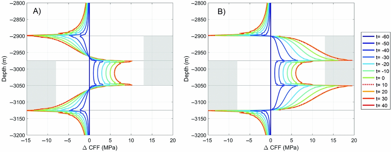
Fig. 17. Finite element model solution for change in Coulomb failure function on the fault assuming reservoir pore pressure (A; cf. Fig. 6A) and Kelvin-chain creep (B).
In Figure 18 we plot the evolution of time-dependent compaction and fault seismic moment density of the Kelvin-chain creep model, normalised to its value at end of production. Furthermore, the moment density has been constructed in accordance with the correlation of compaction strain and the logarithm of seismic moment increase (Bourne et al, Reference Bourne, Oates, van Elk and Doornhof2014, median in their fig. 18a). The time-dependent compaction in Figure 18 for the Kelvin-chain creep is marked by a strong discontinuity after production stop. This is supported by a clear discontinuity in GPS subsidence data in the central area of the Groningen field occurring 9 weeks after production stop (Pijpers & Van der Laan, Reference Pijpers and Van der Laan2016). Markedly, the ratio of seismic moment increase after and before production stop in the geomechanical models is 2–10 times lower and more than 10 times lower than those predicted from the heuristic approach, for the first few years and decades after shut-in respectively (Fig. 18; Van Wees et al., in press). This holds for different creep scenarios ranging from 50 to 500% of non-elastic strain (creep) relative to elastic strain, as well as for both the reservoir and ambient pressure conditions on the fault. The geomechanical predictions are in accordance with the strong reduction of induced events after 80% cut in production rates in the central area in the Groningen field (Fig. 4; Van Thienen-Visser & Breunese, Reference Van Thienen-Visser and Breunese2015; Nepveu et al., Reference Nepveu, van Thienen-Visser and Sijacic2016).

Fig. 18. Left vertical axis: (blue) compaction of the reservoir adopted for the Kelvin-chain creep model. Right vertical axis: (red) seismic moment density normalized to the seismic moment at t=0 using the Bourne et al. (Reference Bourne, Oates, van Elk and Doornhof2014) correlation of compaction strain and seismic moment vs (orange) the moment predicted by the stress changes in the Kelvin-chain creep model. Modified after Van Wees et al. (2017).
The simplified constitutive law for time-dependent compaction and geometry of the model does not allow us to thoroughly assess the sensitivities of the results to variability in geometrical aspects of the reservoir and alternative creep behaviour. However, the prediction of significant reduction of seismicity after cessation of production is expected to hold as well for alternative geometries and constitutive laws, as the first-order effects are determined by the arrest in pressure change (Equation 3).
Conclusions and discussion
We presented the outcomes of geomechanical models against observations of induced seismicity in gas depletion in the Netherlands, with a particular focus on the Groningen field. We focused on the onset and development of seismicity and the reaction due to a production decrease. The prime cause of induced seismicity by gas depletion is stress changes caused by pressure depletion and differential compaction. The observed onset of induced seismicity in the Netherlands occurs after a considerable pressure drop in the gas fields. Geomechanical studies indicate that largest seismicity is likely to be localised on pre-existing fault structures, due to accentuated stress path parameters at faults (Fig. 5). Predicted stress build-up and rupture models show that both the delay in the onset of induced seismicity and the nonlinear increase in seismic moment observed in the induced seismicity can be explained by a model of pressure depletion, if the faults involved in induced seismicity are not critically stressed at the onset of depletion. Upward-concave patterns of log moment with time for individual faults suggest that growth of future seismicity could be more limited than inferred from extrapolating the trend observed between compaction and seismicity to the future (Bourne et al., Reference Bourne, Oates, van Elk and Doornhof2014). The cumulative moment of all rupture models tends to be high compared to observations, which can be explained by the fact that our model neglects the effects of absorption of stress by the salt cap rock and energy losses through aseismic slip. The modelled moment evolution is marked by a concave pattern when plotted on logarithmic scale (Fig. 14). It seems to underestimate the observed more-or-less linear growth of log moment as a function of pressure depletion (Fig. 3) and compaction strains (cf. the partition coefficient in Bourne et al., Reference Bourne, Oates, van Elk and Doornhof2014). Various mechanisms have been proposed which can explain this discrepancy, including the effect of aggregating in time multiple faults with different times of onset of seismicity (cf. Fig. 4), evolutionary effects of rate and state rupture, rate-dependent effects affecting pressures in faults and matrix contributing to seismicity late in the production lifetime of the field.
For time-dependent compaction following a production stop, geomechanical models incorporating Kelvin-chain creep predict that seismic moment increase should slow down immediately after a production stop, independent of the decay rate of the compaction model. These findings are in agreement with low seismicity in the central area of the Groningen field immediately after production decrease on 17 January 2014. The geomechanical model findings therefore support scope for mitigating induced seismicity through adjusting rates of pressure change and production.
The simplified models cannot serve as a comprehensive model for predicting induced seismicity in the Groningen field or any other field. To this end, a more detailed field-specific study, taking into account the full complexity of reservoir geometry, depletion history, and mechanical properties is required. A major challenge for such 3D models is the numerical difficulty of incorporating sufficient resolution and uncertainty for data assimilation and probabilistic predictions. Semi-analytical geomechanical approaches provide a way forward for this challenge, and will be the topic of further study.
Acknowledgements
The data used in this paper are publicly available: seismicity data from the Royal Netherlands Meteorological Institute KNMI (www.knmi.nl); monthly production data from production wells in the Groningen field, available from TNO – Geological Survey of the Netherlands (www.nlog.nl). The Nederlandse Aardolie Maatschappij (NAM) accomplished the original collection of some of the data presented in this paper and is gratefully acknowledged for providing data for Figure 4. The paper benefited considerably from constructive comments from Art McGarr and an anonymous reviewer.


 Open access