


Introduction
Lake Untersee, an oligotrophic, perennially ice-covered freshwater lake in central Dronning Maud Land in East Antarctica, exhibits an unusual thermal structure (Wand et al. Reference Wand, Schwarz, Brüggemann and Bräuer1997). The lake consists of two basins, the northern basin with a maximum reported depth of 169 m is in contact with a glacial wall and is convectively mixed to the bottom (Steel et al. Reference Steel, McKay and Andersen2015), and a second basin to the south is an “anoxic trough”, which is partially shielded from the currents in the main water column (Fig. 1). The lake is ice-sealed, meaning that water does not enter the lake from streams. Instead, melt from the Anuchin Glacier is the primary source of water.
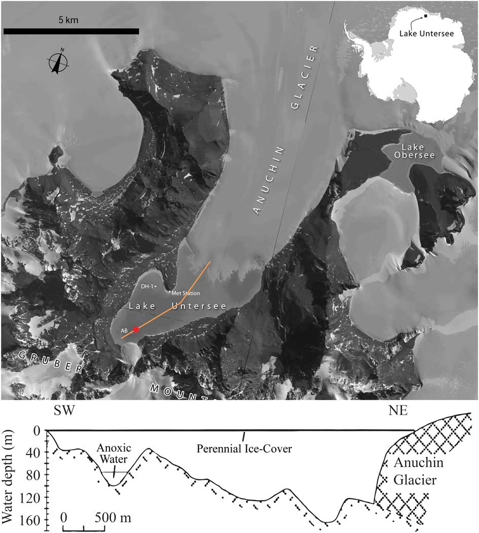
Fig. 1 Satellite imagery and cross-section of Lake Untersee. The cross-section follows the orange line marked on the satellite image. The northern basin is bounded by the Anuchin Glacier which provides a mixing force and thermal sink holding the main lake body near 0 °C. The geometry of the anoxic trough to the southwest end of the cross-section shields the water column from mixing currents in the main body which allows anoxic conditions to persist. The sampling location is marked with a red point. Satellite imagery copyright DigitalGlobe, Inc., provided by NGA Commercial Imagery Program. Profile based on Wand et al. Reference Wand, Samarkin, Nitzsche and Hubberten2006.
An anomalous temperature structure in the anoxic trough was first documented in 1987 (Wand et al. Reference Wand, Schwarz, Brüggemann and Bräuer1997), and the same anomaly has been observed since then (Wand et al. Reference Wand, Samarkin, Nitzsche and Hubberten2006, Andersen et al. Reference Andersen, Sumner, Hawes, Webster-Brown and McKay2011, Steel et al. Reference Steel, McKay and Andersen2015). The temperature profile in the anoxic basin is constant at 0.5°C to 50 m, indicating the depth where shielding from the main basin occurs. At 50 m the temperature increases sharply to ∼4°C, roughly the density maximum of freshwater. Between 50 m and ∼65 m the temperature is constant, implying a convective cell. From ∼65 m, temperature increases linearly to ∼5°C at ∼70 m where it remains constant to ∼80 m. Below 80 m temperature decreases linearly to ∼3.7°C at 100 m depth (Wand et al. Reference Wand, Schwarz, Brüggemann and Bräuer1997) (Fig. 2).
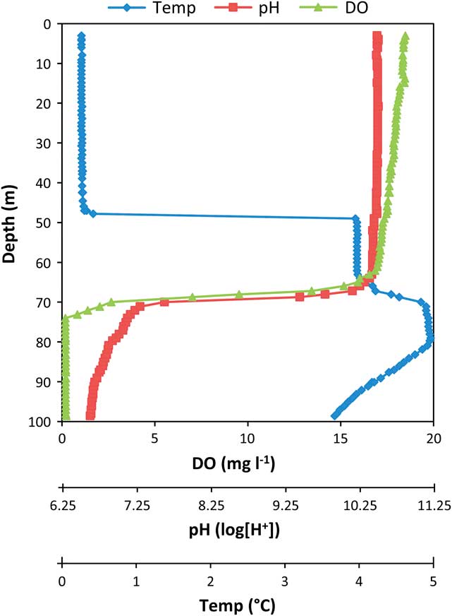
Fig. 2 Profiles of dissolved oxygen, pH and temperature from November 2011. The top portion is well mixed by glacially driven currents above the ridge at ∼50 m. The thermocline at 50 m is well above the oxycline at 68 m where pH and dissolved oxygen (DO) have sharp decreases. Between these depths, the water column is uniform. From 70−74 m is a suboxic region which gives way to anoxic conditions below.
Inverse thermal profiles have been reported in ice-covered lakes in the McMurdo Dry Valleys (Wilson & Wellman Reference Wilson and Wellman1962, Hoare et al. Reference Hoare, Popplewell, House, Henderson, Prebble and Wilson1964, Reference Hoare, Popplewell, House, Henderson, Prebble and Wilson1965, Shirtcliffe Reference Shirtcliffe1964, Bell Reference Bell1967). These thermal profiles have been explained by radiative heating through the lake, and by an increase in salinity with depth, which stabilizes the water column (Wilson & Wellman Reference Wilson and Wellman1962, Shirtcliffe Reference Shirtcliffe1964), even in lakes with very low salinity (Bell Reference Bell1967). Obryk et al. (Reference Obryk, Doran, Hicks, McKay and Priscu2016) demonstrated the importance of solar heating in determining the thermal structure of the perennially ice-covered Lake Fryxell and west lobe of Lake Bonny. In the McMurdo Dry Valleys lakes, temperature plays a minor role in water column stability compared to salinity because temperature ranges are small and they generally overlap with the temperature of maximum density near 4°C (Spigel & Priscu Reference Spigel and Priscu1998). However, water in Lake Untersee is fresh, so salinity is less efficient at stabilizing the water column. In addition, the maximum temperature (5°C) is above the density maximum of water (4°C).
Wand et al. (Reference Wand, Schwarz, Brüggemann and Bräuer1997, Reference Wand, Samarkin, Nitzsche and Hubberten2006) suggested that the thermal increase of 1°C between 70 m and 80 m depth might be explained by microbial metabolism associated with CH4 oxidation, sulfate reduction, and possibly sulfide oxidation, analogous to reports of microbial heating in marine environments (Schwabe & Herbert Reference Schwabe and Herbert2004) and compost heaps and landfills (Pirt Reference Pirt1978). If confirmed, the presence of microbially heated layers in Lake Untersee would be a first in Antarctic limnology.
The aim of this study was to investigate the water column stability and possible thermal sources to explain the unusual temperature profile between 70 m and 80 m depth in the anoxic trough of Lake Untersee. Using field measurements, heating due to absorption of solar insolation through the water column was compared to the theoretical heating derived from chemical energy generation due to aerobic methane oxidation.
Methods
Site description
Lake Untersee covers an area of 11.4 km2 (Loopmann et al. Reference Loopmann, Kaup, Klokov, Simonov and Haendel1988) making it one of the largest lakes in East Antarctica. It has an elevation of 563 m (Andersen et al. Reference Andersen, Sumner, Hawes, Webster-Brown and McKay2011) and average ice thickness of 3 m (Wand et al. Reference Wand, Schwarz, Brüggemann and Bräuer1997). Detailed bathymetry of the lake by Wand et al. (Reference Wand, Schwab, Samarkin and Schachtschneidek1996) revealed that the lake has a large and deep basin in contact with the Anuchin Glacier on the northern edge, which is separated by a narrow sill from the southern end where there is a relatively narrow basin that is not in contact with the shore or with any glaciers (Fig. 1).
The water column in the large basin is well mixed with nearly isothermal temperature profiles and has supersaturated, approximately uniform, concentrations of dissolved oxygen to depths of 169 m. Steel et al. (Reference Steel, McKay and Andersen2015) have shown that the presence of the ice wall of the Anuchin Glacier acts as a heat sink that prevents thermal stabilization of the main basin: water in contact with the glacier wall is cooled below 4°C and as a result is buoyant and rises. The currents driven by this process effectively mix the water column. However, in the smaller southern basin, there is no deep ice to drive convection and the deep and relatively narrow topography blocks these currents, creating stagnant conditions with anoxia developing at depth (Steel et al. Reference Steel, McKay and Andersen2015).
Water column measurements
Four profiles of temperature, depth, conductivity, dissolved oxygen, pH and fluorescence of chlorophyll a (chl a) were obtained using a Hydrolab DS5 multi-parameter water quality sonde (OTT Hydromet, 5600 Lindbergh Drive, Loveland, CO 80539, USA) connected to a field-portable computer. The sonde was factory calibrated four weeks prior to taking each profile, and pH and dissolved oxygen were calibrated in the field before each set of measurements. A 25 cm diameter hole was drilled through the ice to access the water column. Profiles of the water column were obtained on 22 November 2008, 28 November 2011, 5 December 2011 and 1 December 2015. The measurement uncertainty between profiles or casts (instrument uncertainties) was ±0.1°C for temperature, ±1% for conductivity, and ±0.05 m for depth, and it was a factor of two lower for measurements made in the same profile (relative uncertainties from point to point with a cast). The sonde was lowered or raised in 1 m increments and held at each for several measurements. An additional profile of temperature, depth and conductivity was obtained using a RBR concerto (RBR Ltd. 95 Hines Road, Ottawa, ON K2K 2M5 Canada) on 20 November 2016. The sonde was lowered at a rate of 0.13 m s-1 to 50 m, 0.07 m s-1 to the bottom, then raised at a rate of 0.19 m s-1 and had a sampling rate of 3 samples s-1. In the analysis, the 2016 profile was corrected for atmospheric pressure and low salinity in post processing. There is very little variability in the profiles spanning eight years.
Water column stability
Water density profiles were computed from temperature and conductivity profiles where points were binned into 1 m depth brackets (Fig. 3). Comparing repeated scans and upward and downward scans showed that the sampling method was slow enough to prevent hysteresis or memory effects, well below a few percent. In addition, binning minimizes hysteresis effects in the 2016 profile where the sonde was not rested between measurements. The UNESCO formula was used to convert conductivity to total dissolved solids and density (Chen & Millero Reference Chen and Millero1977, Lewis Reference Lewis1980, Millero & Poisson Reference Millero and Poisson1981, Fofonoff & Millard Reference Fofonoff and Millard1983, Chen & Millero Reference Chen and Millero1986, Spigel & Priscu Reference Spigel and Priscu1996, Reference Spigel and Priscu1998, Boehrer et al. Reference Boehrer, Herzsprung and Millero2010). The UNESCO formula is based on seawater, which has a different composition to the water in Lake Untersee. To correct for any errors in density estimation due to this compositional difference, density was directly computed at several depths using direct measurements of the chemical composition of the water (Table 1, Andersen et al. Reference Andersen, Sumner, Hawes, Webster-Brown and McKay2011) and the method of Boehrer et al. (Reference Boehrer, Herzsprung and Millero2010). Data from 95 m depth and below were not used because the density here was calculated to be significantly less than the layer above it. The density profiles computed from the sonde data with the UNESCO formula were then adjusted to agree with the directly computed values. To reach agreement, all profiles were shifted by the addition of a constant 0.034 kg m-3. This offset had no impact on stability analysis, which depends only on relative densities.
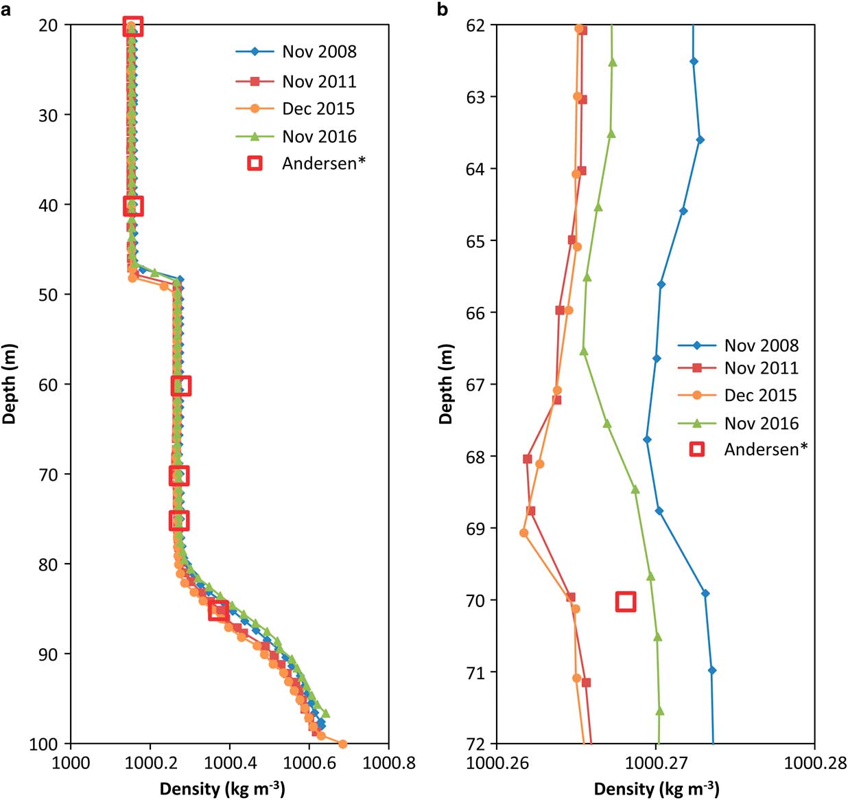
Fig. 3 Density profiles calculated using the UNESCO method shifted to match density calculated using the method of Boehrer et al. (Reference Boehrer, Herzsprung and Millero2010) and data from table 1, Andersen et al. (Reference Andersen, Sumner, Hawes, Webster-Brown and McKay2011). a. The zone above 50 m is connected to the main lake body which is well mixed. The middle zone from 50−68 m which sits between the thermocline and oxycline (chemocline) is a slightly mixed zone. From 68−80 m the column in neutrally stable and below 80 m, stable. b. There is a slight decrease in density from 64−69 m.
Table 1 Summary of energy fluxes, line fits and energy sources * .

* sources assumed to be point layers
Pressure effects on density were not considered because they do not contribute to the stability of stratification (Boehrer et al. Reference Boehrer, Herzsprung and Millero2010). Stability is determined as the difference between the actual density gradient and the gradient in density that would result from an adiabatic lapse rate in density with pressure and temperature. Consequently, in this paper (as in Boehrer et al. Reference Boehrer, Herzsprung and Millero2010) the density was computed with respect to atmospheric pressure, and stability was determined simply as an increase in density with depth.
Thermal analysis
The thermal analysis focused on the region from 70–100 m depth, which was assumed to be fully diffusive with no significant convective transport of heat. Mixing would stop the thermal structure from forming; thus, convection must be a minor component of heat transfer, if it is a factor at all. The thermal gradient was approximated by fitting regression lines to subsections of the measured temperature profiles. These regression lines facilitated numerical calculations by smoothing over noise in the data. The product of temperature gradient and the thermal conductivity coefficient (given as 0.577 W m-1 K-1 by Ramires et al. Reference Ramires, Nieto De Castro, Nagasaka, Nagashima, Assael and Wakeham1995) was used to estimate the thermal flux, and a change in gradient was taken to indicate a location of heat gain or loss. ${\rm Q}{\equals}{\rm k}\left( {{\rm dT}\,/\,{\rm dz}} \right)_{{{\rm upper}}} {\minus}{\rm k}\left( {{\rm dT}\,/\,{\rm dz}} \right)_{{{\rm lower}}}, $
where Q is the heat source, k is the thermal conductivity, T is the temperature, z is depth decreasing downward, and the subscripts “upper” and “lower” refer to segments defined with respect to the location of the heat source. Physically, this is equivalent to summing the fluxes out of a point layer which must be offset by energy input at that layer. For the lower and middle segments all points were included in the analysis, but the upper segment contained artefacts from a convective boundary (Fig. 3b), making determination of the slope of the segment difficult. Thus, the representative lines for the upper segment included only the deepest few points, which were most clearly in the diffusive regime. Fluxes derived from each of the five measured temperature profiles were then averaged.
Chemical and biological heat model
The methane profile reported in Wand et al. (Reference Wand, Samarkin, Nitzsche and Hubberten2006) was used to estimate the possible contribution of metabolic reactions to the water temperature profiles. In particular, Wand et al. (Reference Wand, Samarkin, Nitzsche and Hubberten2006) noted that the methane profile is separated into two regions. From the bottom to 80 m depth the methane concentration was linear with depth, indicating constant diffusion upward without significant loss. From 80 m depth upward to 70 m depth the methane concentration continued to decrease but at a decreasing rate, indicating diffusion upward with loss of methane. Fitting a line to the mostly linear segment from 80 m depth to the bottom provided an estimate of methane flux (slope multiplied by diffusion coefficient) into the consumption zone. To estimate an upper bound on chemical energy generation from methane consumption it was assumed that all consumption was due to oxidation by O2 to CO2 of all methane produced. The flux of methane was determined based on its diffusion coefficient in water of 9.8 × 10⁻⁶ cm2 s-1 at 0.85°C (Yaws Reference Yaws2009). The energy released by the reaction of CH4 with O2 was taken as 890 kJ mol-1 (Weast Reference Weast1976).
Radiative energy heat model
The gradient of the photosynthetically active radiation (PAR) profile was used as the basis for the radiative energy model because longer wavelengths are rapidly absorbed by ice and the first few metres of water (McKay et al. Reference McKay, Clow, Andersen and Wharton1994, Warren & Brandt Reference Warren and Brandt2008). A single profile of radiation in the PAR range (400–700 nm) was measured using a LI-193 spherical quantum sensor (LI-COR, Lincoln, NE 68504, USA) lowered through a hole drilled in the ice cover on 18 November 2011. Measurements were recorded at 5 m increments until 75 m where 1 m increments were used. To normalize the measurements in the water column for changing surface conditions, surface incident radiation was measured simultaneously using a LI-190 cosine corrected sensor (LI-COR, Lincoln, NE 68504, USA) and the percentage of incidence was calculated and used to normalize the underwater measurements. The measured PAR profile represented the proportion of photons in the PAR range reaching a particular depth, which was independent of the surface radiation on the day it was measured. To compute the mean annual radiation at depth, the profile was scaled such that the light level just below the ice at the top of the water column was 2.6 W m-2, is the estimate of the mean annual irradiance as determined from measured surface irradiance, PAR transmissivity, albedo of the ice cover and the theoretical absorption properties of ice over the solar spectrum (Steele et al. Reference Steel, McKay and Andersen2015). It was assumed that photons lost in the water column were completely converted to heat (i.e. negligible conversion to biological or chemical energy). The energy input at each depth was estimated by calculating the slope of the PAR profile.
Results
Water column stability
The temperature, oxygen and pH profiles (Fig. 2), and the computed density profile (Fig. 3), confirmed the existence of four temperature zones, defined below, in the water column of the anoxic trough. This structure was also reflected in the conductivity profiles (Fig. 4).
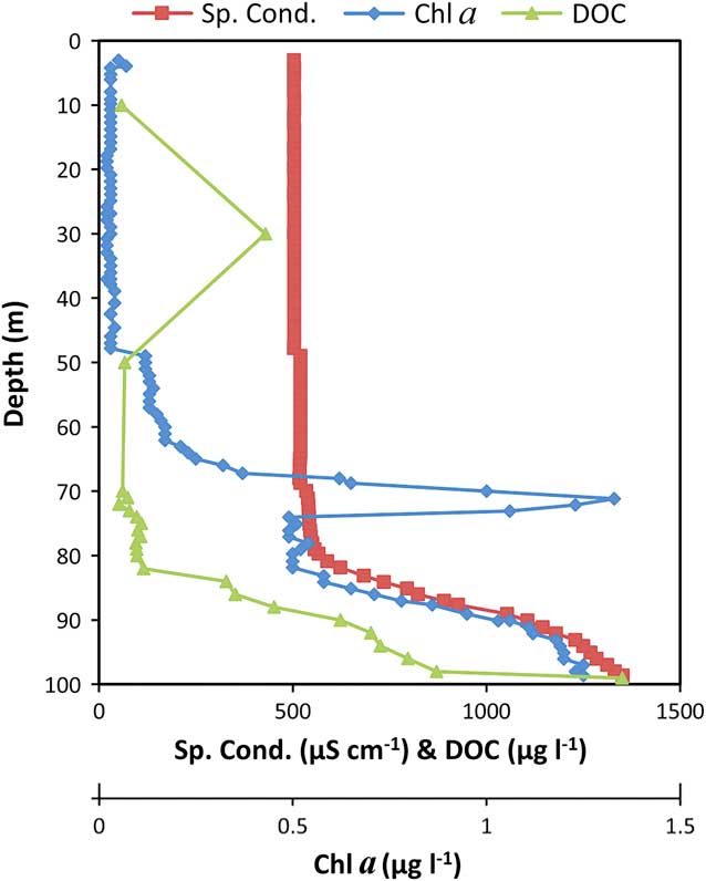
Fig. 4 Profiles of chlorophyll a (chl a), specific conductivity at 25 °C (Sp. Cond.) and dissolved organic carbon (DOC) (Wand et al. Reference Wand, Samarkin, Nitzsche and Hubberten2006) in the anoxic trough. The chl a profile shows a peak at 71.1 m corresponding to a layer of photosynthetic organisms just at the oxycline. The increase in chl a below 80 m may be an artefact of the organic molecules in the water. The conductivity profile shows an increase at 50 m, decrease at 68 m, and rapid increase below 80 m corresponding very closely to the density profile. The dissolved organic carbon profile represents organic molecules in the water column.
The water column was well mixed above the thermocline at 50 m depth. From 50–80 m depth, water density was uniform but higher than the density in the main lake body (Fig. 3). The slope of the density profile indicated that the water column was either mixed or neutral (not mixing but not stable). The chemocline/oxycline was observed within this region (∼68 m depth), which suggests that the water column from 50–68 m depth does not mix with the water column from 68–80 m depth. Below 80 m depth, water density increased to the bottom of the lake. Repeated measurements across eight years revealed identical profiles, suggesting that this portion of the water column must be fully diffusive and stable. A thermal maximum of 5°C occurred 10 m below a column of water at 4°C. This thermal rise could cause instability through a density decrease of ∼0.01 kg m-3, but a slight increase of about 0.012 kg m-3 observed in organic matter in the same zone (Fig. 4) should be sufficient to just stabilize the water column.
There was evidence of a slight unstable slope in density around 65 m depth (Fig. 3b). The persistence of this feature in profiles taken many years apart suggests that it cannot be attributed to sensor noise. When density inversions are very small, conduction is the mode of heat transfer (e.g. Heitz & Westwater Reference Heitz and Westwater1971). To provide a numerical estimate of the strength of convection, the Rayleigh number (Ra) was computed: ${\rm R}_{{\rm a}} {\equals}{\rm \alpha }\Delta \rm TgH^{3} \,/\,\rnu K,$
where α is the thermal expansion coefficient, g is gravity, ΔT, is the temperature difference across the layer of thickness H, ν is the kinematic viscosity and K is the thermal diffusivity. Noting that αΔT is the fractional change in specific volume, v, between the top and bottom of the layer, one can express this in terms of the density, ρ, such that ${\rm \alpha }\Delta {\rm T}{\equals}\Delta {\rm v}\,/\,{\rm v}{\equals}{\rm \rrho }\Delta \left\{ {1\,/\,{\rm \rrho }} \right\}\,\approx\,\Delta {\rm \rrho }\,/\,{\rm \rrho }.$
At 4°C, the kinematic viscosity of water is 1.6 × 10⁻⁶ m2 s-1 and the thermal diffusivity is 1.4 × 10⁻⁷ m2 s-1. From Fig. 3b, density values varied by about 0.002 kg m-3 (hence Δρ/ρ∼2 × 10-6) over a range of ∼1 m. Equations (1) and (2) yielded Ra ∼108, five orders of magnitude higher than the limit for heat transport due exclusively to molecular heat diffusion in horizontal layers with horizontal length scale much larger than the vertical length scale (Heitz & Westwater Reference Heitz and Westwater1971). Ra also exceeded the limit for transition from laminar natural convection to turbulent natural convection (105–106). Our analysis points to a small turbulent convective layer at ∼65 m depth that is persistent over many years but may vary in a location by a few metres.
Thermal analysis
The temperature profiles from 70–100 m depth showed a linear increase followed by a relatively flat plateau at the maximum temperature (5°C) and then a linear decrease (Fig. 5). Given the shape of the temperature maximum, our thermal analysis commenced by fitting three linear segments to the temperature maximum. For most segments, regression lines fitted their respective segments with an R 2 value greater than 0.9. Values of R 2 less than 0.9 were only found in middle segments of December 2011, December 2015 and November 2016. Methodically removing potential visual outliers from December 2011 revealed that the regression line was not strongly affected by these points as the slope and intercept values did not change significantly. The weakness of R 2 as an evaluation of fit quality is acknowledged but given the small number of data points more complex estimators were not practical.
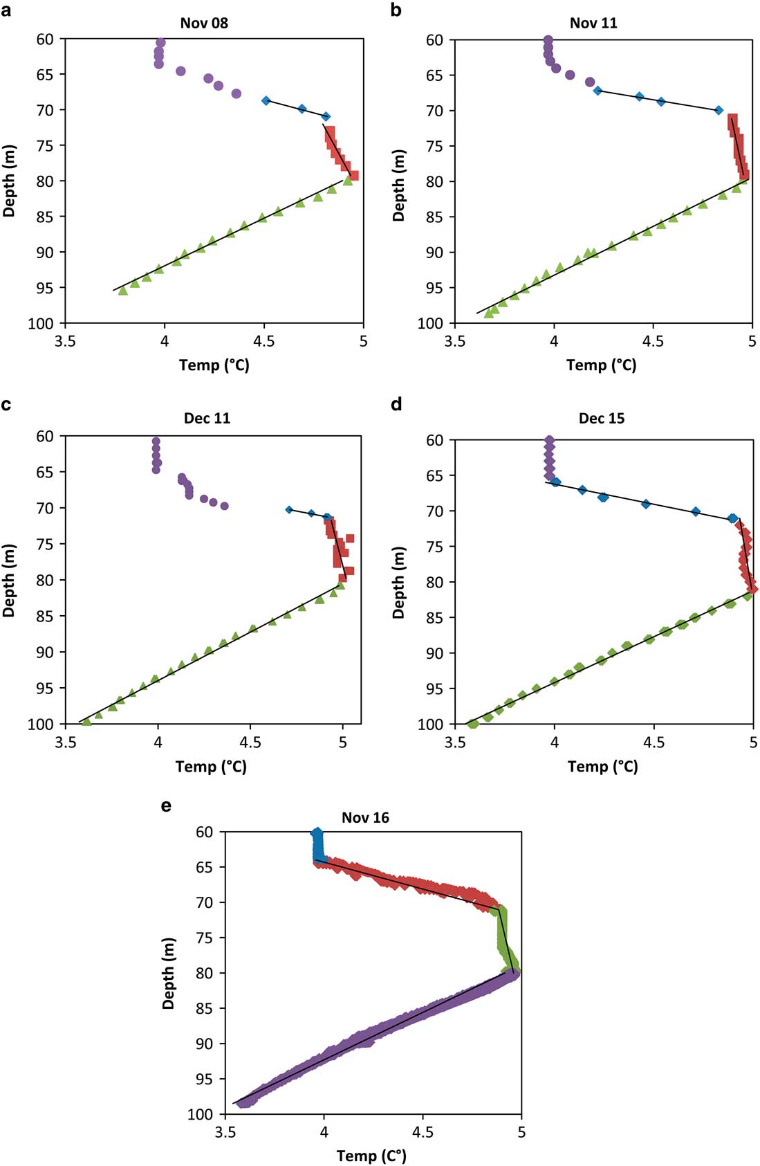
Fig. 5 Temperature profiles and fitted lines from five years. The uppermost points represent the convective transition region above 68 m. The three sections with fitted lines represent the upper, middle and lower segments of the thermal maximum. A noticeable difference is observed in the slope of the upper rise section and convective section where a sharp step occurs in some years. This is probably a result of the small convective layer near 65 m.
Results from all years were very similar to each other apart from the heat flux leaving the upper portion of the temperature maximum. These results are presented in Table I, which shows that the average upward heat flux from the top layer was 0.112 W m-2 and the range for the top was 0.078–0.139 W m-2 - a greater range than that for the other layers (Table I) - and reflects both the numerical resolution of the dataset and the variable physical processes. This upper segment (between ∼65 m and ∼70 m) was affected by the slight instability at ∼65 m depth (Fig. 3b), which resulted in a small convection zone. This convective boundary had an impact on the heat diffused from the layer and might slightly fluctuate in time. The variable magnitude of this upward flux also had a noticeable impact on the total energy requirement because the majority of the energy leaving the temperature maximum system did so from the top. To mitigate the effects of the convective boundary on the energy estimates, only the deepest few points were used in estimating the slope. Values of fluxes and source depths from all years were averaged together, which provided a better approximation than using a single value. Table I contains a summary of the heat fluxes, line fits, energy source depths (segment intersections) and magnitudes for all years. It also includes the averaged energy values used in subsequent sections. The total energy required to maintain the temperature maximum was 0.162 W m-2 and the larger portion was generated by the upper source. The upper source was predicted to be 0.106 W m-2 at a depth of approximately 70.9 m, while the lower source was predicted to be 0.056 W m-2 at a depth of approximately 80.2 m.
Chemical and biological heat model
There are several possible metabolic pathways that could produce energy in this zone of the water column. Of these aerobic methane oxidation is the largest producer of heat because of its high energy yield and the high methane flux through the water column. As discussed above, the linear profile of methane from 80–99 m depth implies a methane flux of ∼1 × 10⁻⁹ mol m-2 s-1 upward from lake bottom. If all of this methane reacted with oxygen to produce carbon dioxide and water, the resulting energy is ∼1 × 10⁻³ W m-2, about 1% of the energy needed to maintain the temperature maximum.
Radiative energy heat model
The bulk of the radiative energy was lost in the upper water column prior to reaching the temperature maximum (Fig. 6). Assuming a 100% conversion from radiative energy to heat, the net radiative flux into the diffusive zone below 70 m, as estimated by the scaled measured PAR profile, was 0.18 W m-2. This was 111% of the radiative flux (0.162 W m-2) required to maintain the temperature maximum given the computed diffusive loss of heat (Fig. 5) and well within the uncertainties of the calculations. In addition, the structure of the energy generation profile (Fig. 6b) had two peaks occurring at 72.5 m and 78.5 m depth, which were similar to the estimated locations from the thermal analysis pointing to heating sources at 70.9 m and 80.2 m depth.
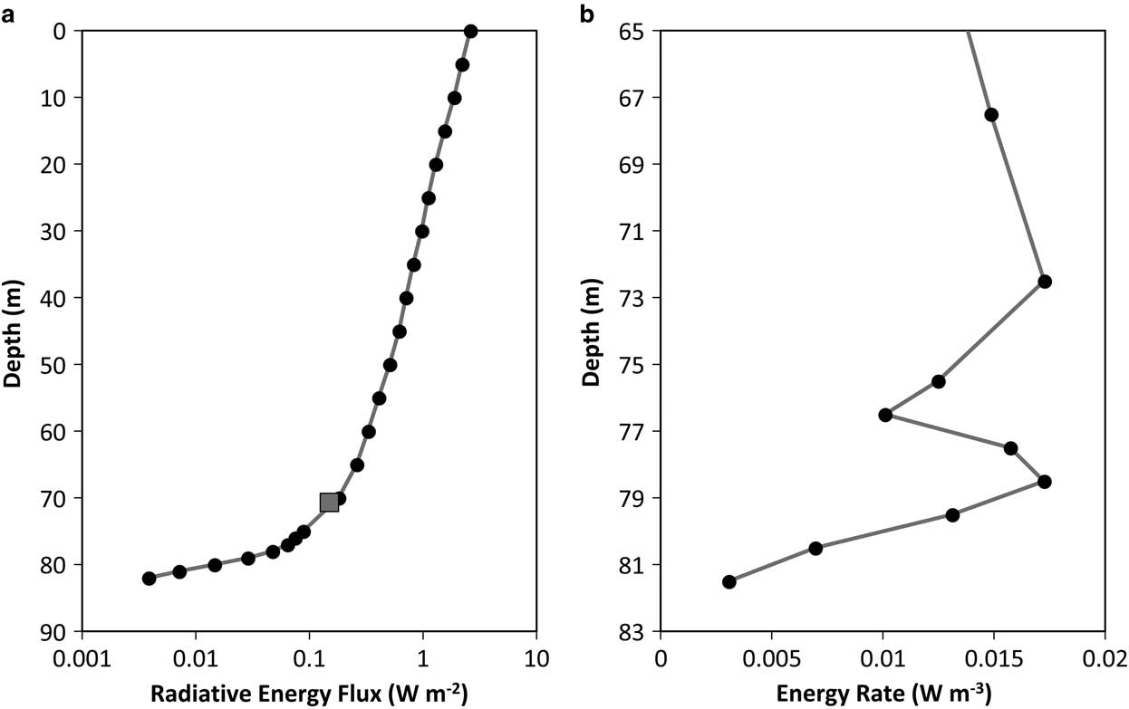
Fig. 6 a. Solar radiation in the anoxic trough scaled by setting the light level just below the ice to 2.6 W m-2, the mean annual irradiance (Steele et al. Reference Steel, McKay and Andersen2015). The square indicates the energy to maintain the thermal rise in the anoxic trough. b. Heating from solar radiation calculated from the slope of the profile. Most of the absorption occurs in the upper portion of the water column. At ∼70 m the profile deviates indicating additional opacity. The heating profile has peaks at 72.5 m and 78.5 m which agree with the predicted values of 70.5 and 79.9 m.
Discussion
Detailed temperature profiles of the anoxic zone span from February 1985 (Wand et al. Reference Wand, Samarkin, Nitzsche and Hubberten2006) to November 2016. Within the spacing of the measurements the structure of the deep temperature profiles are identical, placing a limit on any systematic changes in the level of the lake to <1 m over this two-decade period. In comparison, the level of Lake Vanda increased by 15 m from 1965–2015 (Fig. 4 and Castendyk et al. Reference Castendyk, Obryk, Leidman, Gooseff and Hawes2016) or approximately 3 m dec-1. Above 50 m depth in the anoxic trough, the lake is well mixed from convective currents that are driven by contact with the face of the Anuchin Glacier. This is evident in the uniform profiles above the sill that divides the anoxic trough from the main body at 50 m depth (Steel et al. Reference Steel, McKay and Andersen2015). There is a second mixed zone that sits between the thermocline (50 m) and chemocline (68 m). In this zone the temperature and density are higher than that of the main lake but the dissolved oxygen concentration is essentially the same. This suggests that the convective mixing in this zone can transport enough dissolved oxygen to maintain its concentration equal to the value in the upper layers of the lake. The mixing also maintains isothermal conditions, but apparently the mixing is not strong enough to keep the temperature equal to the temperature of the water in the upper layers of the lake, ∼0°C and the water is warmed to 4°C. This is probably due to the stability of water at its density maximum, 4°C, favouring this value of the temperature. There is no corresponding effect on the level of dissolved oxygen. However, just above the chemocline there is a small instability between 64 m and 69 m depth where density appears to decrease slightly (0.005 kg m-3). Stability through the profiles arises from an increase in salt concentrations, which offsets density changes from increasing temperature over the density maximum of water. In Antarctic lakes Vanda and Bonney, salts are the primary component to stability (Wilson & Wellman Reference Wilson and Wellman1962, Shirtcliffe & Benseman Reference Shirtcliffe and Benseman1964, Spigel et al. Reference Spigel, Priscu, Obryk, Stone and Doran2018). Though Lake Untersee has very low concentrations of salts compared to those systems, dissolved salts are also the stabilizing agent (table 2 in Wand et al. Reference Wand, Samarkin, Nitzsche and Hubberten2006 & table 1 in Andersen et al. Reference Andersen, Sumner, Hawes, Webster-Brown and McKay2011).
From the shape of the temperature profile (Fig. 5) it is clear that the heating structure required to explain the thermal maximum is more complex than in other Antarctic lakes that also show temperature rises with depth. The energy flux of 0.162 W m-2 required to explain the temperature maxima (71 m) is 5–10 times lower than estimated values for other Antarctic lakes, such as Vanda (Wilson & Wellman Reference Wilson and Wellman1962), Miers (Bell Reference Bell1967), and Bonney (Shirtcliffe Reference Shirtcliffe1964). One possible explanation for this difference is the magnitude of the temperature anomaly, which in the case of Lake Untersee is only 1°C while the anomalies in other lakes are much larger. As discussed above, a single distributed source does not adequately approximate the observed profile. Instead, two thin layers at 70.9 m and 80.2 m depth that act as point sources of heat in the water column are required to explain the profile. In the remainder of the paper and in Table I these will be referred to as point layers.
The thermal analysis provides boundaries and guidance for evaluating plausible energy sources to explain the temperature profile (Wand et al. Reference Wand, Samarkin, Nitzsche and Hubberten2006). The maximum heating from metabolic reactions (i.e. methane oxidation) is several orders of magnitude smaller than the energy required to cause the observed raise in temperature. Methane oxidation is the single largest chemical contributor to heating because of the high concentration of methane in the water column and a high-energy yield. Thus, one can conclude that chemical and biological reactions are not the primary heating source.
The dominant energy source is solar heating through the water column. In the case of Lake Untersee, the estimated radiative input of 0.18 W m-2 through the water column was 111% of the energy flux required to explain the temperature maxima. The discrepancy (11%) between estimated radiative input values and required radiative input values is similar to other studies in Antarctic lakes (Wilson & Wellman Reference Wilson and Wellman1962, Shirtcliffe Reference Shirtcliffe1964) and falls within the 20% error that is commensurate with the methods used in this analysis. However, the absolute discrepancy in the case of Lake Untersee (0.018 W m-2) is 3–5 times smaller than the 0.066 W m-2 reported by Wilson & Wellman (Reference Wilson and Wellman1962) and 0.106 W m-2 reported by Shirtcliffe (Reference Shirtcliffe1964) for Lake Vanda.
Energy input peaks are predicted from the solar radiation profile at 72.5 m and 78.5 m depth (Fig. 6b), which are similar to the estimates of 70.9 m and 80.2 m from the thermal analysis. The location of the upper peak is in a section where sampling resolution was 5 m for most of the profiles, so there is a large error associated with the true location. The lower peak is within a section of 1 m sampling resolution but occurs within 2 m of the estimated location, which given the uncertainty in the data is in good agreement.
The upper temperature point layer would receive a higher solar radiation flux, and only a relatively small portion of that solar radiation flux would need to be converted into heat to explain the observed change in temperature. The chl a profile from 2011 showed a distinct peak at the same location as the upper temperature peak (Fig. 4) and was similar to the profile of dissolved organic carbon reported by Wand et al. (Reference Wand, Samarkin, Nitzsche and Hubberten2006). This suggests that there is a high density of phytoplankton at this depth, which is located at the chemocline/oxycline. However, photosynthesis alone is probably not capable of converting this radiative energy into heat, because the energy used by the phytoplankton in Antarctic lakes is only 3–8% of the incoming radiative energy (Seaburg et al. Reference Seaburg, Kaspar and Parker1983). Instead, it is more likely that photosynthesis is a source of energy that supports the growth of phytoplankton and that the phytoplankton and the microbial community that it supports acts as a source of opacity in the water. A similar mechanism of heating is probably active in Lake Vanda (Wilson & Wellman Reference Wilson and Wellman1962, Vincent et al. Reference Vincent, Rae, Laurion, Howard-Williams and Priscu1998).
The lower thermal generation point layer would receive a solar radiation flux equivalent to 10% of the solar flux at the upper peak. Thus, the water column must be more opaque at the lower peak for a more efficient heat conversion. It is likely that this lower heat-absorbing layer is from particulate organic and/or inorganic matter and not from chl a, as it occurs at the depth where methane oxidation and sulfate production reach maximum values (Wand et al. Reference Wand, Samarkin, Nitzsche and Hubberten2006). Again, the depth spacing in our data makes precise determination of the location impossible, but it is plausible that there is a layer of chemotrophic microorganisms at this depth that are supported by chemical species in the water column. This microbial-rich layer and other associated organic molecules could act as a source of opacity to convert incoming radiative energy to heat (Markager & Vincent Reference Markager and Vincent2000, Thrane et al. Reference Thrane, Hessen and Andersen2014). Interestingly, the depths of the upper and lower heat peaks coincide with the upper and lower boundaries of the suboxic zone defined by Wand et al. (Reference Wand, Samarkin, Nitzsche and Hubberten2006). The top of this zone is the oxycline while the bottom is a transition to fully anoxic conditions.
The timescales required to generate the observed thermal profile can be estimated by dividing the amount of energy required to heat the water column by the observed energy flux into the water column. The time required to heat the water column below the well mixed zone at 50 m depth to the bottom at 100 m from 0°C to the first temperature step (4°C) by solar radiation (0.45 W m-2, as seen in Fig. 6) is approximately 60 years. The time required to heat the water column at the second temperature step (4–5°C) from 62–92 m from the predicted energy input (0.16 W m-2) is ∼14 years. This timescale is shorter than the 25-year time period for which the thermal rise has been observed suggesting that the heating mechanisms is active at the current time. The fact that it takes only 14 years to create a 1°C rise in temperature is also noteworthy because it shows how quickly the structure of the anoxic trough could change should solar radiation at depth increase as a result from changes in climate or lake level. Changes in the deep thermal structure of this magnitude over ∼80-year timescales have been reported for Lake Vanda (Castendyk et al. Reference Castendyk, Obryk, Leidman, Gooseff and Hawes2016).
Lake Untersee may be a sensitive indicator ecosystem for climate change. Andersen et al. (Reference Andersen, McKay and Lagun2015) found that a 1°C rise in mean air temperature would result in meltwater flowing down the Anuchin Glacier leading to the formation of runoff channels on the glacier, moats around the lake, and the introduction of dissolved CO2 into the water column. This in turn would drive down pH leading to the precipitation of carbonates and silicates. Streamflow derived from glacial runoff would dramatically increase the load of fine sediments transported into the extremely transparent water column. In this regard, it is interesting to note that the thermal structure of the anaerobic basin may dramatically alter in response to changes in the radiation balance of the surface of the lake and the opacity of the upper water column. The profiles over 20 years provide a baseline record of long-term stability.
Conclusion
Lake Untersee has a thermal structure that is unusual among ice-covered Antarctic lakes, due to the geometry of the lake and the resultant formation of an anoxic trough. The main lake body and the larger basin are all well mixed, isothermal and uniformly saturated with dissolved oxygen. The anoxic conditions in the trough persist because of the deep yet narrow geometry, which shields the water from mixing currents. There are distinct zones in the water column of the anoxic trough. The upper zone (0–50 m) is part of the main lake body and connected by current-driven mixing. The zone from 50–68 m is slightly mixed and maintains a separation of the oxycline from the thermocline. The zone from 68 m to the bottom at 100 m is purely diffusive and has an unexpected thermal temperature rise of 1°C. The structure of the profile in this region is best reproduced with two discrete sources acting at different depths. The top source coincides with a photosynthetic layer just at the oxycline while the second source overlays the depth where peak methane oxidation and sulfate reduction rates occur. While metabolic reactions could account for only 1% of the required energy, solar radiation can account for 111% of the required energy. Thus, heating of the anoxic basin is more likely due to these microbial populations acting as sources of opacity, which converts solar radiation into heat.
The stability of the temperature maximum is maintained by dissolved solids in the water column, which are most likely dissolved salts in low concentrations. The thermal rise in Lake Untersee is different from those found in Lake Vanda and Lake Bonney by being deeper, smaller in the maximum temperature, but similar in that stability is maintained by dissolved salts.
The combination of physical setting, a glacier wall, which induces mixing, topography of the anoxic trough that shields the basin to the mixing, and the depth of the anoxic trough, make Lake Untersee unusual among Antarctic lakes. These features result in a diffusion zone and the formation of an oxycline and chemocline. Biological entities respond to the availability of oxidants and reductants at the chemocline by creating biomass. This leads to opacity in the water, which then absorbs solar flux creating a thermal maximum.
Our analysis shows that the structure of the thermal profile depends on the penetration of surface radiation. If future climate change results in a change in solar radiation this will directly affect the thermal profile.
Acknowledgements
Primary support for this research was provided by the Tawani Foundation, the Trottier Family Foundation, the Arctic and Antarctic Research Institute/Russian Antarctic Expedition’s Subprogram “Study and Research of the Antarctic” of the Federal Target Program “World Ocean”, and NASA’s Astrobiology Program. Logistics support was provided by Antarctic Logistics Centre International (ALCI), Cape Town, South Africa. We are grateful to Colonel (IL) J. N. Pritzker, IL ARNG (retired), Lorne Trottier, and fellow field team members for their support during the expedition. The authors also thank Robert Spigel and a second anonymous reviewer for constructive comments on the text.
Author contributions
JB developed the conceptual model of heating and density stability. All authors contributed to the writing and analysis. Field work was conducted by DTA, CPM, AD, IH and YT.
Supplemental data
The raw data used in this manuscript are freely available as an excel file at https://doi.org/10.1017/S0954102018000354. The file includes data from various Lake Untersee column profiles for temperature conductivity, pH, Dissolved oxygen and light; and data used for water density and thermal flux calculations.


 Open access