


Introduction
Early high-frequency radar studies in alpine snowpacks indicated that the technique has great potential, particularly by facilitating spatially and temporally continuous measurements. Relatively few studies exist, however, when compared with oil exploration, road and building infrastructure, geotechnical engineering, and glaciology applications. Thus quantitative interpretation of radar measurements in snow remains challenging, as few inversion techniques have been developed for estimating snowpack properties. Conversely, snow is an advantageous medium, as excavation and ground-truth measurements can be made relatively quickly and easily.
Reference Vickers and RoseVickers and Rose (1973) first described the use of impulse radar (2–7 GHz) in an alpine snowpack for measuring snow stratigraphy at high resolution. Commercially available impulse radars have been used to accurately estimate total snow water equivalent (SWE) to 5–10% (Reference Sand and BrulandSand and Bruland, 1998; Reference Lundberg, Thunehed and BergströmLundberg and others, 2000). Reference Harper and BradfordHarper and Bradford (2003) recently made detailed measurements in a 20m × 20 m study plot and found good general agreement between detailed manual density profiles and the lower-resolution density profile estimated from a common midpoint (CMP) inversion (three modeled layers in 250 cm).
Reference Ellerbruch and BoyneEllerbruch and Boyne (1980) first published frequency-modulated continuous wave (FMCW) radar results for alpine snow. They identified ground and surface reflections, estimated SWE at many sites to ±5%, observed a strong reflection from a depth-hoar layer, and measured changes in the surface reflection during a day when the surface snow experienced some melting. In the early 1980s, Reference Gubler and HillerGubler and Hiller (1984) developed an FMCW system to measure the speed and heights of avalanches, and also were able to measure mean density ![]() to within ±5%. Gubler and Weilenmann (1987) made static measurements while removing layers sequentially from the surface, and also qualitatively compared FMCW radar measurements with ram and morphological profiles.
to within ±5%. Gubler and Weilenmann (1987) made static measurements while removing layers sequentially from the surface, and also qualitatively compared FMCW radar measurements with ram and morphological profiles.
In 1982, Reference Fujino, Wakahama, Suzuki, Matsumoto and KuroiwaFujino and others (1985) developed an FMCW system for use in alpine snow, and made both laboratory and continuous static field measurements. They found that correlating reflections with layer interfaces was difficult, and therefore inserted metal plates at layer interfaces as markers, but did not do any calculations with these measurements. Reference Forster, Davis, Rand and MooreForster and others (1991) made measurements of snow stratigraphy in the upper 6 m of a site at the Upstream B camp, West Antarctica, with an X-band FMCW radar. They observed reflections from depth-hoar/wind-crust pairs which were interpreted as annual layers, allowing calculation of accumulation rates. Reference Gubler and RychetnikGubler and Rychetnik (1991) present FMCW profiles that indicate significantly less snow layering in forest stands than in open fields.
Conditions that lead to an increase or decrease of snowwetness are of considerable interest to snow remote-sensing and avalanche formation, prompting Reference Koh and JordanKoh and Jordan (1995) to show that FMCW radar is capable of detecting small melt events. They combined FMCW measurements with the snowpack model SNTHERM, and observed subsurface melting on a calm, clear day when temperatures were near
but not above, freezing. The one-dimensional mass- and energy-balance model was able to reproduce the evidence of near-surface melting from the FMCW measurements. Reference Koh, Yankielun and BaptistaKoh and others (1996) made measurements at three different frequency ranges (C-, X- and Ka-bands) and showed that a multiband approach is required for FMCW measurements in a wide range of snowpack conditions. They state that this type of FMCW system has great potential for profiling stratigraphy, depth, SWE and for monitoring liquid water content, but found that signal interpretation remains challenging. Reference Holmgren, Sturm, Yankielun and KohHolmgren and others (1998) used an X-band FMCW system similar to that used by Reference Koh, Yankielun and BaptistaKoh and others (1996) to investigate the accuracy of making snow-depth measurements. They found the system usually reproduced snow depth accurately, but the ground reflection was sometimes ambiguous, which they attributed to an irregular ground surface and orientation of the antennas. Reference Kanagaratnam, Gogineni, Gundestrup and LarsenKanagaratnam and others (2001) have developed an FMCW system to map internal layers in Greenland, which they correlate with electrical conductivity measurement (ECM) recordings from an ice core.
Theory
FMCW radar
Because the accuracy of estimating target distance is inversely proportional to bandwidth B, broadband FMCW radars offer an advantage over impulse radars, without requiring a digital-to-analog converter with a high sample rate. The broad bandwidth possible with an FMCW system (≥4 GHz) results in a greater theoretical vertical resolution (δz ≈ 3 cm) compared to commercial impulse radars (δz ≈ 17 cm) which have a typical bandwidth B < 700 MHz. Although the highest frequencies are strongly attenuated by liquid water, we have always been able to identify ground reflections at our lowest frequency range (2–6 GHz), in snowpacks up to 3.5 m deep.
The FMCW technique has been described elsewhere (e.g. Reference StoveStove, 1992), and here we provide just a brief summary. A sinusoidal chirp waveform, whose frequency varies linearly with time for the duration of the pulse T pl, is transmitted. A sample of the transmitted pulse is mixed (i.e. multiplied) by the received signal before data acquisition, yielding a signal whose frequency spectrum contains the frequency differences between the two signals. The linearity of the frequency of the two signals forces the frequency difference Δf to be constant over the entire bandwidth B, and this difference is proportional to the two-way travel time T 2w to any given target. The distance d to a given target can be calculated if the velocity of propagation in snow v s is known:

where ![]() is the velocity of electromagnetic waves in snow, c = 3.0 × 10⁸ (m s-1) is the speed of light in a vacuum and
is the velocity of electromagnetic waves in snow, c = 3.0 × 10⁸ (m s-1) is the speed of light in a vacuum and ![]() is the mean dielectric constant of snow.
is the mean dielectric constant of snow.
Dielectric properties of snow
In the microwave frequency range, the dielectric constant of snow є depends on density ρ s and wetness W (e.g. Reference Ulaby, Moore and FungUlaby and others, 1981). Various empirical and physically based models have been proposed for dry snow (W ∼ 0), as shown in Figure 1. Because we do not have enough data yet to develop our own dielectric model, and since differences in the published models (Fig. 1) may result from differences in instrumentation (Reference Schneebeli, Coléou, Touvier and LesaffreSchneebeli and others, 1998), we perform our calculations with each model and indicate the range of results they produce.

Fig. 1. Dielectric properties of dry snow.
Estimating SWE
Four different methods have been used for estimating SWE from radar measurements. Each method uses radar measurements of the two-way travel time T 2w, calculated from difference in time between the reflection from the snow surface and that from the ground. This depends on both the velocity of propagation v s (which depends on density and wetness) and the snow depth d s
The first method, a strictly empirical approach, uses a linear fit to SWE measurements and radar T
2w at several control sites, and then assumes this relationship remains constant along a traverse (Reference Sand and BrulandSand and Bruland, 1998). Reference Lundberg, Thunehed and BergströmLundberg and others (2000) use a second method, which consists of measuring mean snow density ![]() at a few representative sites to estimate v
s, and assumes
at a few representative sites to estimate v
s, and assumes ![]() remains constant along a traverse. The radar measurements yield T
2w which can be used with v
s to calculate snow depth d
s and
remains constant along a traverse. The radar measurements yield T
2w which can be used with v
s to calculate snow depth d
s and ![]() where ρ
w = 1000 (kgm–3) is the density of water.
where ρ
w = 1000 (kgm–3) is the density of water.
The third method, described by Reference Ellerbruch and BoyneEllerbruch and Boyne (1980) and Gubler and Hiller (1984), uses the opposite technique, where snow depth d
s is measured and mean density ![]() is calculated from T
2w. Since the two-way travel time T
2w is much more sensitive to snow depth d
s than mean density
is calculated from T
2w. Since the two-way travel time T
2w is much more sensitive to snow depth d
s than mean density ![]() this technique is more prone to errors, but measuring d
s is much faster and can be done at a higher spatial density. The fourth method, described by Reference Gubler and WeilenmannGubler and Weilenmann (1986), uses an FMCW radar buried underneath the snow, and a corner reflector mounted above the snow surface. This technique can only be used at a fixed site, and produces accurate SWE estimates for thick snow covers with a SWE of >100 mm. Since we are interested in a method of estimating SWE in a wide range of snowpacks and along profiles rather than at fixed sites, below we discuss the accuracy of each of the first three methods.
this technique is more prone to errors, but measuring d
s is much faster and can be done at a higher spatial density. The fourth method, described by Reference Gubler and WeilenmannGubler and Weilenmann (1986), uses an FMCW radar buried underneath the snow, and a corner reflector mounted above the snow surface. This technique can only be used at a fixed site, and produces accurate SWE estimates for thick snow covers with a SWE of >100 mm. Since we are interested in a method of estimating SWE in a wide range of snowpacks and along profiles rather than at fixed sites, below we discuss the accuracy of each of the first three methods.
Methods
In our experiments we compare the FMCW radar signal to measurements we made using several more established techniques. We evaluate measurements at five different sites, where at each site we make radar measurements complemented by standard manual profiles which include measurements of layer hardness, grain-size and type, temperature, and density in a freshly excavated snow pit. The Finnish Snowfork (Reference Tiuri, Sihvola, Nyfors and HallikainenTiuri and others, 1984) was also used to make in situ measurements of the complex dielectric constant ![]() in the wall of the pit at 2 cm vertical intervals. The snow fork allows a higher-resolution density profile than can be made with manual measurements, and also gives quantitative information about the in situ dielectric properties that the FMCW radar responds to.
in the wall of the pit at 2 cm vertical intervals. The snow fork allows a higher-resolution density profile than can be made with manual measurements, and also gives quantitative information about the in situ dielectric properties that the FMCW radar responds to.
Finally, we inserted a thin piece of steel horizontally at all major layer interfaces, and then made static FMCW measurements. The steel caused obvious large reflections, which were used to identify the precise location within the snowpack of reflections in the original radar measurements, to calculate the average dielectric properties of the snow between the reflector and the surface, and to determine the accuracy of the previously calculated depth scale, which used just an average velocity for the entire snowpack.
Results
Measurements were made during winter 2002/03 at five sites, with SWE ranging from <18 to >90 cm, as part of the NASA Cold Land Processes (CLPX) Mission (Reference ClineCline, 2000; Reference Marshall, Koh and ForsterMarshall and others, 2004). We begin by using the two-way travel time T 2w within each snowpack to estimate SWE as described above. Then as an example, we compare the FMCW signal with detailed manual and in situ measurements at one site.
Snow water equivalent (SWE)
A vertical profile of manual density measurements was made at each site, where 100 cm3 samples were collected every 5 cm and weighed, and the measured SWE was calculated by integrating this profile. We developed an algorithm to automatically pick the surface and ground reflections from each radar dataset, and then calculate the two-way travel time T 2w between the two. We model the SWE at each site using each of the first three methods described above, and for each method the SWE is estimated using each of the dielectric models in Figure 1.
Table 1 lists the error associated with each method, and the variability depending on the dielectric model chosen (Fig. 1), for snowpacks with a SWE of 17–95 cm. Note that the first method (empirical T
2w models) has the highest variability depending on the model chosen, and indicates that, if this method is used, a local calibration is required. Since the propagation velocity is not extremely sensitive to density, using a measurement of mean density ![]() is much more accurate than using a measurement of depth. In addition, snow depth is much more spatially variable than mean snow density. Using just a typical dry snow density at all sites
is much more accurate than using a measurement of depth. In addition, snow depth is much more spatially variable than mean snow density. Using just a typical dry snow density at all sites ![]() still gives a reasonably accurate value (error <10%), while having the advantage of using the radar data alone.
still gives a reasonably accurate value (error <10%), while having the advantage of using the radar data alone.

Fig. 2. Comparison of measured and modeled SWE. A vertical manual density profile was integrated to calculate the measured SWE, and the modeled SWE was found by using a typical dry snow density of ![]() The vertical error bars indicate the error caused by choice of dielectric model when using radar measurements combined with a depth measurement, and the horizontal error bars indicate the estimated uncertainty in the measured SWE.
The vertical error bars indicate the error caused by choice of dielectric model when using radar measurements combined with a depth measurement, and the horizontal error bars indicate the estimated uncertainty in the measured SWE.
Table 1. SWE estimates. ‘Error’ shows the calculated error eachmethod had with our data, and ‘Model var.’ indicates the variability of the result due to the choice of dielectric model used

Figure 2 shows the SWE estimates, and the solid line indicates a perfect agreement between measured and modeled SWE. The circles show the results at each of the five sites using ![]() and the squares indicate the agreement between the SWE estimated from the two-way travel time to the metal reflectors and the integrated density profile above these reflectors. The error associated with the choice of dielectric model is within the size of the symbols for this method, and the error associated with the method of using a depth measurement is shown with the vertical error bars. The horizontal error bars indicate the estimated error in our measured SWE (10%).
and the squares indicate the agreement between the SWE estimated from the two-way travel time to the metal reflectors and the integrated density profile above these reflectors. The error associated with the choice of dielectric model is within the size of the symbols for this method, and the error associated with the method of using a depth measurement is shown with the vertical error bars. The horizontal error bars indicate the estimated error in our measured SWE (10%).
Comparison with manual and in situ measurements
Radar reflections from the snow surface and the ground can be used to estimate the total SWE. In this detailed example, we show in addition that the internal snowpack reflections mark major transitions in density and hardness. Figure 3a shows the measured hand hardness shaded in gray, along with the density profile (black circles) at the Local Scale Observation Site (LSOS) in the Frasier Experimental Forest on 28 March 2003. Grain-size and type are indicated on the left.

Fig. 3. (a) Manual snow pit showing visually identified layers, with hand hardness shown in gray (scale on top), and manual density measurements shown with circles (scale on bottom). Grain-size and type are indicated on the left. (b) In situ reflectivity calculated from snow-fork measurements. (c) Mean FMCW radar signal near snow pit. (d) FMCW radar measurements with metal reflectors at the surface, 48 and 56 cm.
In order to compare the radar measurements with the in situ electrical measurements, since the radar responds to changes in electrical properties, we calculate the in situ reflectivity Γ
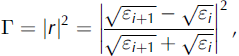
where єi +1 єi are the complex dielectric constants at the adjacent depths z i+1, zi . Figure 3b shows the in situ reflectivity Γ measured with the snow fork, and Figure 3c shows the average radar measurement. The radar signal shows an obvious surface reflection (z = 0), a reflection from the near-surface wind crust at z = 10 cm, three clear reflections between 30 and 60 cm depth near density and hardness transitions observed in the pit, two smaller reflections at 70 and 80 cm, and a clear ground reflection at 110 cm. Note that all but one of the reflections from within the 110 cm snowpack occur within 5 cm of regions of large reflectivity Г. This correlation is within the accuracy of the radar and the error in the co-registering of the two measurements, and confirms that the radar responds to the in situ electrical properties of the snowpack that were measured with established methods.
Metal reflector experiments
The depth scale for the radar measurement used above was calculated using the mean snowpack density ![]() neglecting that the velocity of propagation v
s is different within each layer. To investigate the error due to this assumption, measurements were made with a steel reflector placed at several well-defined layer interfaces. Figure 3d shows results with metal reflectors in the snowpack. The solid black line indicates a measurement with the reflector at the surface, and the dashed and gray lines show the result of the reflector placed at 48 and 56 cm, respectively. These two depths mark major layer interfaces observed in the snow pit. At z = 48 cm, there is an increase in density, hardness and grain-size, and at z = 56 cm there is a decrease in density, hardness and grain-size.
neglecting that the velocity of propagation v
s is different within each layer. To investigate the error due to this assumption, measurements were made with a steel reflector placed at several well-defined layer interfaces. Figure 3d shows results with metal reflectors in the snowpack. The solid black line indicates a measurement with the reflector at the surface, and the dashed and gray lines show the result of the reflector placed at 48 and 56 cm, respectively. These two depths mark major layer interfaces observed in the snow pit. At z = 48 cm, there is an increase in density, hardness and grain-size, and at z = 56 cm there is a decrease in density, hardness and grain-size.
The location of the metal reflector is obvious in the radar measurement, as the reflection is at least 20 dB above any other signals in each case, and agrees with the approximate depth scale to within 2 cm. The theoretical resolution of this radar, with a bandwidth B of 4 GHz, is 3.12 cm using the mean density ![]() for this particular snowpack. In addition, note that the measurement made before the snow pit was excavated (Fig. 3c) shows reflections at the same locations, indicating that the radar is responding to these changes in density and hardness.
for this particular snowpack. In addition, note that the measurement made before the snow pit was excavated (Fig. 3c) shows reflections at the same locations, indicating that the radar is responding to these changes in density and hardness.
Figure 4 shows the actual depth of the reflector as a function of the observed radar T
2w for measurements with the reflector at z = 0, 48, 56, 66.5, 74.5 and 100 cm. The slope of the dashed line is the mean velocity between each reflector, and the slope of the gray line indicates the mean velocity calculated from ![]() The location of each metal reflector can be estimated from the radar measurement to within 2 cm using this mean velocity, so using the mean density to estimate the mean velocity of propagation is quite accurate. These measurements clearly demonstrate that radar reflections occur within the snowpack at layer boundaries that can be visually identified in a nearby snow pit. The FMCW system therefore has the potential to be very useful for avalanche research, by detecting major changes in density and hardness that can be monitored along profiles in avalanche-prone terrain.
The location of each metal reflector can be estimated from the radar measurement to within 2 cm using this mean velocity, so using the mean density to estimate the mean velocity of propagation is quite accurate. These measurements clearly demonstrate that radar reflections occur within the snowpack at layer boundaries that can be visually identified in a nearby snow pit. The FMCW system therefore has the potential to be very useful for avalanche research, by detecting major changes in density and hardness that can be monitored along profiles in avalanche-prone terrain.

Fig. 4. TWT of large reflections caused by metal reflectors at various known depths.
FMCW profile
Using this approximate depth scale, an image of a radar scan at 2–6GHz is shown in Figure 5. This image is shown with a scale from white to black, where white indicates no reflection and black indicates a very strong reflection. This measurement was made by sweeping the radar horn antennas from left to right over a 3m distance, and then back again. This was done by hand, and every attempt was made to move the antenna horns at constant velocity. Therefore, the data from the left side of the image to the middle should approximate a mirror image of those from the middle to the righthand side. A large degree of variability exists within 3 m at this flat, wind-protected site, and more importantly this variability is repeatable (variability on left half can also be seen in approximately the same location on the right half). The measurement was repeated six times, and each produced a similar result. Note also the reflections on the lefthand side (nearest the snow pit), at ∼10, 48, 56, 70 cm, and the ground at 110cm are well correlated with transitions observed in the nearby snow pit (Fig. 3a), and indicate that significant variations in layer geometry and density can occur on a length scale of <3 m.

Fig. 5. FMCW radar scan, 2–6 GHz. Dark areas indicate strong reflections; light areas indicate no reflection. Distance scanned is approximately 3 m (trace 0–250). Measurement was made from left to right and then back again, illustrating the spatial variability present and the repeatability of the measurement.
Conclusion
FMCW radar provides a promising tool for measuring and monitoring snowpack stratigraphy and SWE. In agreement with previous radar work in alpine snowpacks, we have successfully measured SWE with an error of ∼10% when combined with a measurement of snow depth. The choice of dielectric model used has a large (∼10%) effect on the result when using this method, and thus may be a major cause of the error. We calculated SWE at each site using all of the models shown in Figure 1, producing results that range from the model of Reference Schneebeli, Coléou, Touvier and LesaffreSchneebeli and others (1998), which has the highest R 2 value (0.988), to the model of Reference MatzlerMatzler (1996), which agrees very well with theory. The variability in these models has been attributed to the instrument used, so a dielectric model developed from radar measurements may improve SWE estimates when using the method of combining radar and manual depth measurements.
When the radar measurement is combined with a measurement of the mean density ![]() (Reference Lundberg, Thunehed and BergströmLundberg and others, 2000), we can calculate SWE with an error of <2%, although this method is more time-consuming. Assuming the mean density
(Reference Lundberg, Thunehed and BergströmLundberg and others, 2000), we can calculate SWE with an error of <2%, although this method is more time-consuming. Assuming the mean density ![]() is always 250 kgm–3 still provides a useful estimate, with an error <10% for our measurements. Because the propagation velocity is not highly sensitive to density, the choice of dielectric model used produces much less uncertainty with these methods compared to using a depth measurement.
is always 250 kgm–3 still provides a useful estimate, with an error <10% for our measurements. Because the propagation velocity is not highly sensitive to density, the choice of dielectric model used produces much less uncertainty with these methods compared to using a depth measurement.
We also compared our radar measurements at one site with detailed in situ dielectric measurements, showing that the radar reflections occur near large changes in dielectric properties. Measurements made with metal reflectors inserted at layer interfaces located the cause of major reflections in the initial measurement, and showed that using a mean velocity for the snowpack introduces a vertical depth error of <2 cm.
We present the results of a 3 m scan at 2–6 GHz, which shows major reflections occurring near layer interfaces identified manually in the nearby snow pit. This scan also shows large, repeatable variations, indicating that variations in density and/or hardness may occur on length scales less than 1 m, similar to recent results from snow penetrometer measurements by Reference Kronholm, Schweizer and SchneebeliKronholm and others (2004). The ability to measure the degree of spatial variability is important for avalanche studies, as it strongly influences the avalanche formation process (Reference Kronholm and SchweizerKronholm and Schweizer, 2003), but this has been difficult in the past with the traditional, time-consuming techniques. This work shows that an FMCW radar can effectively measure SWE of an alpine snowpack, and that major transitions in density and hardness can be detected and their variations monitored along traverses.
Acknowledgements
The manuscript was greatly improved by the comments of S. O’Neil, M. Sturm, H. Conway and an anonymous reviewer. K. Elder and D. Cline helped facilitate the field measurements.


