


Introduction
Black Rapids Glacier is a surge-type temperate valley glacier located along the Denali fault in the Alaska Range of interior Alaska, U.S.A. It is 42 km long with an average width of 2.3 km and a mean slope of 2° (Fig. 1). Black Rapids Glacier last surged in 1936/37 and has been the subject of intensive field study from 1970 to the present (see in particular Reference Heinrichs, Mayo, Echelmeyer and HarrisonHeinrichs and others, 1996). The main trunk of the glacier makes a hairpin turn near the equilibrium line, but aside from this bend, it flows obliquely away from and later directly towards the European Remote-sensing Satellite-1 and-2 (ERS-1/-2) synthetic aperture radar (SAR) cross-track imaging direction, in the accumulation and ablation areas, respectively, making it an excellent subject for study using interferometric SAR (InSAR) (Reference Goldstein, Engelhardt, Kamb and FrolichGoldstein and others, 1993; Reference JoughinJoughin, 1995; Reference Joughin, Kwok and FahnestockJoughin and others, 1996a, Reference Joughin, Tulaczyk, Fahnestock and Kwokb; Reference Rignot, Forster and IsacksRignot and others, 1996; Reference Fatland and LingleFatland and Lingle, 1998,Reference Fatland and Lingle2002). Black Rapids Glacier has two other large tributaries just above its equilibrium line, each leading to an ice divide. The first is the divide with East Fork Susitna Glacier to the southwest, and the second is the divide with Susitna Glacier proper, to the west along the Denali fault (Fig. 2a). This second tributary extends only 4 km west from Black Rapids to the Susitna divide, where it is in turn fed by a steeper unnamed tributary to the north (nominally designated “Melville” herein). The Susitna tributary is of interest in this study because of an anomalous motion signal in the interferometric image phase that persists for at least 78 days in early 1992, and which appears again faintly in InSAR data from early 1996.

Fig. 1. Black Rapids Glacier, Alaska Range, interior Alaska. Lower right inset indicates glacier location. Upper right indicates glacier outline and principal tributaries, echoed by bold lines on the main figure. (UTM grid is a 10 km grid.)

Fig. 2. (a) Sar image of black rapids glacier with feature labels. tri is the “melville”tributary flowing into sus, susitna glacier, at the ice divide. efs is the east fork susitna tributary, also with ice divide indicated. acc is the accumulation area. numerical transect labels (8, 14, 17, etc.) are longitudinal distances from the head of the glacier. transect bars correspond to the plots in (b). abl indicates the upper ablation area. lok is the loket tributary, with its intrusive medial moraine loop visible in the sar image.

Fig. 2. (b) Lateral glacier-speed profiles from early 1992 (dashed lines) and late 1995 (solid lines). The direction sense of each profile is shown by compass labels at the plot extremes.
Before discussing this anomaly, we describe the derivation of surface velocity vector fields on Black Rapids Glacier from single-orbital-path InSAR. InSAR ice-velocity derivation uses multiple interferometric pairs under the assumption that the velocity field remains constant for the duration of two sequential observation periods, an assumption usually more valid for polar ice sheets than for temperate valley glaciers. Multiple pairs are used to isolate the motion signal from the topographic signal (see Reference Kwok and FahnestockKwok and Fahnestock, 1996; Reference Fatland and LingleFatland and Lingle, 1998). Failure of this constant-velocity assumption introduces errors and can highlight interesting dynamic behavior of the glacier, as described below. The principal SAR observations used herein are from winter 1991/92 (3 day repeat orbits using ERS-1) and from winter 1995/96 (1day repeat orbits using ERS-1/-2 tandem-mission image pairs). Data accuracy and errors are discussed throughout, with emphasis on the recurring theme of high local relative accuracy in contrast with lower absolute accuracy.
Surface Ice-Velocity Pattern
Methods
The derivation of a glacier surface velocity vector field from a single orbit path requires flow-direction information in addition to interferometric phase. This is in contrast to the preferred method where both ascending and descending orbit-path InSAR data are available (Reference Joughin, Kwok and FahnestockJoughin and others, 1998). Over larger regions of continuous ice such as on ice sheets, flow-direction unit vectors in the horizontal plane are obtained from image co-registration and speckle tracking. In the present case where the area of interest is relatively small (tens of pixels), a scheme for generating these unit vectors was adopted that makes use, instead, of known flow directions, constrained by valley walls and indicated by medial moraines. This method can be a useful alternative to co-registration “speckle tracking” for small areas with complex but fairly stable flow patterns.
We assume that flow along the surface is in the direction parallel to the glacier’s constraining valley walls (Reference Fatland and LingleFatland and Lingle, 1998). Flow direction for tributaries and confluences is determined by a spatially compartmentalized best-guess technique, with guidance from field data, image feature tracking, and moraines that can be treated as flow-lines. Once the flow-direction field is defined, the interferogram phase is translated to a radial distance vector pointing from the ice to the SAR, and this is in turn projected into the surface-tangent flow-direction vector. The result is divided by the observation time interval to produce a velocity vector field. Variations in glacier speed on a scale of days to weeks are the primary contributor to error in the derived velocities (see below). Flow-direction estimate errors and errors in interferometric baseline give second-order velocity errors.
Observations
Figures 2 and 3 show graphical representations of the Black Rapids Glacier surface velocity field. Data gaps both at the main Black Rapids Glacier bend near the equilibrium line and in the Loket tributary are due to orientation of the ice flow parallel to the SAR flight track (InSAR is least sensitive to this direction of flow). The longitudinal velocity profile in Figure 3b shows the expected extensional and compressional flows in the accumulation and ablation areas, respectively. Superimposed on this trend is a 50% (8 cm d−1) slow-down of the main glacier over about 2 km above the Loket tributary confluence. Continuing downstream, the velocity “recovers” immediately after the Loket confluence. The distance over which this slow-down occurs corresponds to 3–4 ice thicknesses, in good agreement with the longitudinal coupling scale suggested by Reference Kamb and EchelmeyerKamb and Echelmeyer (1986).

Fig. 3. (a) Black Rapids Glacier velocity profiles overlain on the SAR image of the glacier. (b) Inset shows a longitudinal profile down the center of the glacier. (c) Speed contour plot. Invalid data regions noted where glacier flow parallels flight path. (d) Proxy strain-rate details.
Figure 2b shows 17 transverse velocity profiles from the accumulation area (8 km) down-glacier to 10 km above the terminus (32 km). The southern margin profiles undergo a transition from parabolic shape, indicative of deformational flow (8 km group), to steep lateral gradient plug-flow shape (14–20km). Further downstream they transition again, back to parabolic shape above Loket tributary. In contrast, the profiles for the heavily debris-covered northern margin are consistently parabolic, with an outer inflection indicating stagnant ice.
The 1995/96 InSAR observations spanned a 67 day period from 1995-351 to 1996-056 (year-day). Survey cameras emplaced on the glacier margins at the 14 km site give a center speed increase of 20% from 9 to 11 cm d−1. The 20 km survey site speed increased from 11to 14 cm d−1, where errors are estimated at ±2 cm d−1. For purposes of precise comparison with InSAR, we used spot measurements of flow direction from Reference HeinrichsHeinrichs (1994), including positive emergence velocities. The InSAR average velocities were 12 and 10 cm d−1, respectively. This supports the contention that variations in temperate glacier flow velocity can lead to errors in the InSAR-derived speed, discussed further in the next subsection.
Error analysis
The objective of this analysis is to quantify errors in glacier surface speed estimation as derived from single-orbit-path differential InSAR. High-frequency signal noise and baseline estimation errors make relatively small contributions relative to the three main sources: variations in surface velocity, fixing the zero-velocity reference, and errors in estimation of flow direction.
Surface velocity variation errors
We consider two constitutive interferograms with a small relative variation in surface velocity. We take an ice motion
![]() resulting in a radial motion change ΔR to be reflected in the phase of the first interferogram. The second interferogram is produced from ice moving by
resulting in a radial motion change ΔR to be reflected in the phase of the first interferogram. The second interferogram is produced from ice moving by
![]() resulting in a radial distance change (ΔR + δR). The two interferogram phases are approximately
resulting in a radial distance change (ΔR + δR). The two interferogram phases are approximately

Here k is the SAR carrier-signal wavenumber, R the mean slant range, α the radar beam incidence angle, and h the terrain elevation. The Bi are respective interferometric baselines, where by writing the second as a scaling of the first, B 2 = FB 1, we can write the differential motion-only phase as
For two identical baselines, F = 1, and steady ice motion δR = 0, the motion signal vanishes. As B 2 varies from B 1 the proportional influence of δR changes accordingly. That is, if ΔR corresponds to a “correct” velocity v ΔR and δR is written as a fraction of ΔR, δr = EΔR, then from ψmotion we will calculate an “incorrect” velocity
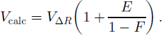
For example, using B 1 = 200 m and B 2 = 20 m with a velocity perturbation of 10% (E = 0.1), V calc will be in error by 11 %. However, we are free to reverse the baseline order, B 1 = 20 m and B 2 = 200 m, which reduces the error to 1 %. This legerdemain simply reflects the way InSAR baseline-dependent topographic sensitivity weights the differential motion signal. Ideally, the entire issue is avoided by using a single interferogram and a sufficiently accurate topographic model, but failing this solution, the effects of surface velocity variability can be accounted through some combination of multiple datasets and ground truth.
Zero-velocity reference-point errors
A Zero-velocity reference is the pixel phase over stationary terrain. It is used as a seed-point in extrapolating the velocity field across a nearby glacier where the terrain is moving. In this work, the Zero-velocity phase at the glacier margin for 1 day repeat data (ERS tandem mission) had an uncertainty of about 2% of one fringe (2π/50 rad). This value, when projected into the velocity field, gives an error of 1 mm d−1 for horizontal-plane motion in the direction of the SAR cross-track direction. As the flow-direction angle increases from 0° up to 75° relative to this axis, the error increases to 5 mm d–1 . (Surface motion at an angle > 75° is difficult to resolve using single-orbit-path InSAR data.)
Flow-direction and incidence-angle estimation errors
Two angles relate surface motion to SAR imaging geometry: the azimuthal (map projection) flow-direction angle θ relative to the SAR cross-track direction, and the radar-beam incidence angle α relative to the local flow direction. The latter value should properly include the emergent component of the ice motion, although this will be a small correction to the calculated velocity. The two angles θ and α relate the ice flow in three-dimensional space to the one-dimensional SAR look-axis. They can therefore be used to convert interferometric phase (i.e. path-length change ΔR along the look-axis due to ice motion
![]() to ice speed s via
to ice speed s via
where ΔR = -φ/2k and ΔT is the repeat-pass time interval. Glaciers flow approximately parallel to their constraining valley walls, with slight divergence in ablation areas and convergence in accumulation areas when considered in traverse from the center of the glacier to the margin. Flow directions are further complicated by variations in the bed and by the influence of tributaries (Reference RaymondRaymond, 1971; Reference EchelmeyerEchelmeyer, 1983). Here we estimate a combined worst-case flow direction error of 8°, giving velocity errors of about 15% in the Black Rapids Glacier accumulation area, 5 % in the plug-flow region above the Loket tributary moraine, and 2% below the moraine where the flow direction is closest to ideal.
Error summary
Consideration of all error sources gives an absolute velocity uncertainty of ∼20% on the Black Rapids Glacier accumulation area and ∼15% on the ablation area. This absolute error is due to changes in glacier speed between interferometric observation intervals and errors in estimation of flow direction, including surface slope and emergent velocity factors. Although 20% errors in absolute speeds are large, InSAR analysis does much better at showing relative aspects of glacier surface motion, for example through one-dimensional transverse and longitudinal profiles. Multiple-orbit-path analysis (when possible) will fare better, with the caveat that the time-varying velocity of temperate glaciers will contribute errors to any multiple-observation-interval based measurement.
Strain rates
Using a surface velocity vector field discussed above, it is straightforward to use the spatial derivative (∂u/∂x,∂u/∂y) as a proxy for the two-dimensional surface strain-rate field in which vertical strain is neglected (after Reference VaughanVaughan, 1993). On Black Rapids Glacier the maximum observed principal strain rate, found in the shear margins, is about 2.5×10⁻⁴ d−1 (Fig. 3d). Strain rates approximated in this manner are not subject to errors in absolute velocity.
Local Motion Anomalies
Observations
1992 InSAR images of the Susitna tributary to Black Rapids Glacier (Fig. 2a: SUS) contained an unusual localized phase pattern, prompting further investigation. Figure 4a shows an “expected” phase signal, no anomalous motion, from ERS-1/-2 tandem-mission data acquired in 1995. The phase in this image indicates very little ice motion over the course of 1day (1995-351/352, baseline 156 m). That is, most of the phase signal on the glacier is due to topography. The Susitna and East Fork Susitna ice divides are indicated with dashed lines in both Figure 4a and b, and the Melville tributary that flows north to south into the Susitna tributary at the ice divide is also labeled. Figure 4b, from late 1996 tandemmission data (27 m baseline), shows the same region with two faint motion anomalies marked with dashed lines. The first is on the Black Rapids accumulation area and is lakelike in shape. The second is associated with the east side of the Melville outlet into the Susitna tributary, just on the Black Rapids side of the Susitna divide.

Fig. 4. Two winter 19 95/96 interferograms of the Black Rapids Glacier equilibrium-line region, including the East Fork and Susitna tributaries and the Melville tributary. Upper image shows motion phase combined with glacier topography phase but no trace of the winter 1991/92 motion anomaly. This anomaly is, however, faintly visible in the lower image, emphasized with a dotted line. Another possible anomaly in the ablation area is similarly indicated.
The faint Susitna anomaly would be easy to dismiss were it not for the 1992 InSAR data. A series of 13 InSAR image pairs spanning 78 days show a persistent “bull’s-eye” pattern in the same location. These patterns have bigger amplitudes and vary in shape and position (Fig. 5). The center of the pattern (white dots) migrates fairly steadily over time out into the center of the ice channel and downstream towards Black Rapids. Figure 5l and n briefly reprise this migration at the end of the sequence from 1992-061 through 1992-070. In all cases, the phase curvature of the motion anomaly indicates that the center is moving towards the SAR with time. The anomalies have a typical diameter of about 2 km, elongated along the glacier flow direction, and each has a clear association with the Melville tributary, particularly its southeast corner.

Fig. 5. (a–m) a time sequence of winter 1991/92 interferograms in the black rapids glacier equilibrium-line area. labels give start times (year-day), insar repeat intervals (3 or 6 days) and baselines. white dots show center locations of the anomalies, summarized in ( n) as a migration path. ( n) also shows flow directions and the two ice divides “d”. the bar graph shows the vertical motion uplift at the bull’s-eye centers for each 3 day time interval.
Interpretation
We begin by defining three distinct interpretive frames for analyzing single-orbit-path InSAR phase signals. InSAR phase measures a one-dimensional radial component of three-dimensional motion, along the SAR line of sight. For typical glacier motion, one assumes the ice moves approximately within the horizontal surface plane, as described in the above section on velocity derivation. This assumption defines the standard interpretive frame for InSAR phase in terms of the normal flow of the glacier down-valley. In the standard interpretive frame, the SAR line-of-sight component of motion is projected into a near-horizontal glacier flow vector field to derive surface ice speed. A second interpretive frame, the vertical motion interpretive frame, ignores horizontal-plane motion and ascribes a phase signal to localized rise and fall of the surface ice. Vertical movement is a less common and less intuitive glacier phenomenon. Between these first two interpretive frames lies a third: a synthesized or combined interpretive frame in which the InSAR phase is attributed to some combination of vertical and horizontal motion.
The Susitna tributary motion anomalies can be interpreted as localized speed-up in horizontal flow using the standard interpretive frame (horizontal motion only). However, incompressibility of ice immediately necessitates a transition to the combined (horizontal + vertical) interpretive frame, since compression/extension longitudinally across the bull’s-eye expanse will change the ice thickness by a SAR-observable amount (cm). The question of which interpretive frame is correct is left open here, but this initial observation implies that some vertical motion is part of these anomalies, i.e. we are reduced to a choice between combined and vertical-motion interpretive frames.
If we adopt the vertical-motion interpretive frame to analyze the Susitna tributary anomalies, the nature of the motion/signal relationship is simplified. In this case, the surface of the glacier moves vertically upward by 3.1 cm for every fringe (2π rad) relative to the surrounding ice, but this introduces the physical problem of how several hundred meters of ice are going up like a slow elevator for 78 days in the middle of winter. To address this problem, we refer to temperate-glacier motion anomalies seen from InSAR phase of other glaciers.
In the case of bull’s-eyes found on the stagnant terminus ice of both Bering and Malaspina Glaciers, south central Alaska (Reference Fatland and LingleFatland and Lingle, 2002), a clear link has been established between the motion anomalies and subglacial hydrology.We suppose that on Black Rapids Glacier, by analogy, some mechanism increases the water pressure under the Susitna tributary to exceed the overburden pressure of the ice. Tending to further increase the overburden pressure would force more water under the glacier, raising the glacier surface as implied by the vertical-motion interpretation of these anomalies. Themechanismby which this could happen is not clear, but may be hinted at by the geometry of the situation: the Susitna tributary lies at the bottom of a long south-facing tributary (Melville) and sits below the Aurora Peak catchment to the north. It is conceivable that an aquifer or subglacial conduit exists with sufficient hydrological head to drive the hypothesized hydraulic jacking.
This hypothesis has interesting implications for subglacial hydrology. The migration of the anomaly down-glacier at about 30 m d− 1 implies a sort of creeping subglacial lake that grows over the course of mid-winter as it slowly makes its way downstream under the ice. Thevolume growth can be estimated from the interferometric phase by approximating the anomalous region as a conical volume and summing across 78 days of data, interpolating the missing values (see Fig. 5, bar chart). In this case, the vertical uplift over 3 days is approximately 3 cm per fringe, and the fringes are counted in both upstream and downstream directions and averaged to remove the local phase gradient bias. This calculation gives an average basal water influx rate of 0.23 m3 s−1.
An incident related to this implicit water-storage capacity occurred during a field campaign on Black Rapids Glacier in April 1996 (well before the onset of surface melt). Water was pumped from a 600m deep borehole (Fig. 2a, 14 km) with a water level 80 m below the surface (a hydraulic head at 96% of the overburden pressure). A total of 3000L of water, the approximate equivalent of the total borehole volume, were removed from the borehole in 20 min with no noticeable change in this water level. Later, 1000L were pumped back into the borehole in the same amount of time with the same result, indicating that the borehole was connected to a considerable aquifer.
The frequent initiation of surges in early winter seems to imply that a surging glacier must be capable of storing a substantial amount of water subglacially, after the end of the melt season. In support of this idea, observations on Gornergletscher, Swiss Alps, show hydraulic uplift to be the dominant component of vertical surface motion (Reference Iken, Fabri and FunkIken and others, 1996).
Discussion
We maintain that there are two prima facie equally valid interpretive frames for understanding the phase signal for the Black Rapids motion anomalies presented here. The vertical-motion interpretive frame is the simpler of the two and implies high subglacial water storage consistent with data from this and other glaciers. Thecombined (horizontal +vertical) interpretive frame does not require high subglacial water pressure but would necessitate a mechanism for the increase in horizontal motion during winter. A strictly horizontal-motion-based interpretation (standard frame) is ruled out as being physically unlikely.
Based on the larger body of interferometric glacier data we have processed, we favor the vertical-motion interpretive frame, which raises the interesting problem of how a large hydraulic head is established and maintained at the base of the glacier, apparently pumping 1.6×10⁶ m3 of water under the glacier over the course of 78 days. The interferogram time sequence of Figure 5 covers only 45 of these 78 days, but each interferogram indicates a surface rise, so lowering events during this time period seem unlikely; we surmise that the surface was continuously inflating. This notion of continuous inflation suggests an obvious connection to surge initiation, which also occurs in the middle of winter. We can speculate, for example, that the 1992 migrating-phase bull’seye sequence may have been the signature of a nascent surge initiation (glacier–bed decoupling) that dispersed before reaching a necessary critical instability. If the recurrence on a smaller scale in the 1995 data indicates a commonly recurring phenomenon, then it would be of interest to emplace global positioning system data recorders to unambiguously resolve the nature of the motion in question.
Conclusions
Building accurate velocity maps for temperate glaciers is quite feasible using single-orbit-path InSAR data with good absolute results (520% error) and very good relative speed measurements ( ≤ 4% error). This is best done using a very accurate elevation model, but in lieu of that, differential InSAR (two observation intervals) can be used to remove topography from the total phase signal. The residual signal, attributed to “standard interpretive frame” motion (i.e. downstream in the plane of the glacier surface), is affected by variations in the glacier speed over the constitutive time intervals. Beyond the basic procedures of InSAR processing, the majority of the work involved in velocity-field calculation consists in the generation of a reasonable flow-direction unit vector field. Strain-rate calculations are also easily made and are unaffected by errors in absolute velocity.
In the course of developing this procedure, a series of interferograms were found with phase that does not mesh easily with the standard interpretive frame, suggesting both the vertical- and the combined-motion interpretive frame. The combined-motion frame allows for localized regions of fast-moving ice. However, when these are treated as transient phenomena as indicated by the data, there must be an associated thickening of the ice due to volume conservation, hence the horizontal motion is combined with a vertical-motion component. This interpretive frame raises the problem of a mechanism to accelerate a circular mass of ice at the center of the glacier (bull’s-eye center) in such a way as to produce circular rings of phase.
In contrast, the vertical-motion interpretive frame is simpler to apply to the phase signal of these anomalies, and is also consistent with known cases of strict vertical motion on stagnant glacier termini elsewhere. An interesting possible implication, consistent with field observations on Black Rapids Glacier, is that water at the glacier bed is held at a pressure equal to or slightly above the ice overburden pressure and is behaving in mid-winter like a gradually growing, creeping subglacial lake. The source of this water might be an aquifer or conduit coupling the area to water stored at higher elevation. Since the anomaly is faintly apparent in 1996 data, it is reasonable to assume it is a fairly common occurrence, and perhaps represents a type of bid for surge initiation.
Acknowledgements
The authors would like to thank W. D. Harrison and K. A. Echelmeyer for valuable discussion and suggestions during the course of this work. This work was supported through the NASA ADRO program.We also thank our editor T. A. Scambos, an anonymous reviewer and C. F. Raymond for considerable assistance in preparing this paper.


