


INTRODUCTION
Accurate estimates of the mass balance of Antarctic ice grounded above flotation are important for constraining projections of global sea level rise. Accumulation of snow provides positive input to the mass balance, while Antarctica loses mass through wind-driven ablation, sublimation and discharge across the grounding line. The largest loss of ice is due to ice flowing across the grounding line into the floating ice shelves. These ice shelves provide an important buttressing back stress (Dupont and Alley, Reference Dupont and Alley2005) on the fast-flowing ice streams and glaciers, and their removal can lead to rapid ice stream acceleration (Scambos and others, Reference Scambos, Bohlander, Shuman and Skvarca2004) and sea level rise.
The removal of mass from ice shelves occurs through calving of icebergs from the terminus and melting at the ice shelf base. The amount of mass loss through basal melting is thought to be greater than that from calving, but estimates vary between studies (e.g. Depoorter and others, Reference Depoorter2013; Rignot and others, Reference Rignot, Jacobs, Mouginot and Scheuchl2013; Liu and others, Reference Liu2015). Iceberg calving can be observed from satellites and so its contribution to the Antarctic mass budget can be quantified (Liu and others, Reference Liu2015). Access to the ocean-filled cavity beneath ice shelves and measuring basal melting in situ is logistically difficult; sea ice impedes access from the open ocean; and, surface access through borehole drilling leads to sparse observations. Estimates of basal melting from satellite rely on assumptions, which can often limit accuracy (spatially and temporally) on small-scales. Ice shelf/ocean models allow small- and regional-scale interaction to be studied, leading to improved understanding of the physics involved, better wide-scale surveys of basal melt and improved estimates of Antarctic ice sheet mass budget for projecting sea level rise.
Ocean water above the in situ freezing point (which decreases with increasing pressure) melts ice at depth, producing a buoyant meltwater plume that can refreeze at shallower ice; thermohaline circulation produces vertical overturning circulation. This mechanism was described as an ‘ice pump’ (Lewis and Perkin, Reference Lewis and Perkin1986). Jacobs and others (Reference Jacobs, Hellmer, Doake, Jenkins and Frolich1992) expanded upon this and proposed three modes of melting: mode (1) dense water melts at depth and the resultant thermohaline circulation can produce refreezing at shallower locations (like the ‘ice pump’ mechanism), mode (2) warm water inflow at intermediate depth and mode (3) relatively shallow melting near to the ice front. The commonly used method for parameterising this melting takes into account the availability of heat and salt, and the magnitude of currents, which turbulently mix warmer ocean water to the ice/ocean interface (Holland and Jenkins, Reference Holland and Jenkins1999). The parameterisation indicates melting will occur where there is water substantially above the in situ freezing point and where an ocean current exists. Holland and others (Reference Holland, Jenkins and Holland2008) found melting to be proportional to the product of driving from water currents and temperature at the ice shelf base, and both to increase linearly with far-field ocean temperature. Hence, melt rate increases quadratically with ocean temperature. Little and others (Reference Little, Gnanadesikan and Oppenheimer2009) suggest that inefficiencies in converting entrained heat into melting increase as temperature is increased, and therefore the ocean temperature/melt relationship will be less-than-quadratic but greater-than-linear.
The sub-ice shelf oceanic environment can be divided into two broad classifications of ‘cold cavity’ or ‘hot cavity’ by the relative temperature of the inflowing water, following Joughin and others (Reference Joughin, Alley and Holland2012). Hot ocean cavity environments are roughly defined by water well above the in situ freezing point flowing beneath the ice shelf and driving strong melting with an area-averaged melt of ${\rm {\cal O}}(10)\;{\rm m}\;{\rm a}^{ - 1} $
. The archetypical hot ice shelf cavity is beneath the Pine Island Ice Shelf, where strong melting is driven by Circumpolar Deep Water nearly 4°C above the in situ freezing point (Jacobs and others, Reference Jacobs, Jenkins, Giulivi and Dutrieux2011). Cold ocean cavity environments are characterised by water having a temperature close to the surface freezing point entering the ice shelf cavity and driving weaker basal melting with an area-averaged melt of
${\rm {\cal O}}(10)\;{\rm m}\;{\rm a}^{ - 1} $
. The archetypical hot ice shelf cavity is beneath the Pine Island Ice Shelf, where strong melting is driven by Circumpolar Deep Water nearly 4°C above the in situ freezing point (Jacobs and others, Reference Jacobs, Jenkins, Giulivi and Dutrieux2011). Cold ocean cavity environments are characterised by water having a temperature close to the surface freezing point entering the ice shelf cavity and driving weaker basal melting with an area-averaged melt of ${\rm {\cal O}}(0.1 - 1)\;{\rm m}\;{\rm a}^{ - 1} $
. In the cold cavity environment, ascending buoyant meltwater can produce supercooling, frazil formation and significant marine ice accretion. Ice shelves that fit this classification include the Larsen C Ice Shelf and the three largest ice shelves, the Ross, Filchner-Ronne and Amery ice shelves.
${\rm {\cal O}}(0.1 - 1)\;{\rm m}\;{\rm a}^{ - 1} $
. In the cold cavity environment, ascending buoyant meltwater can produce supercooling, frazil formation and significant marine ice accretion. Ice shelves that fit this classification include the Larsen C Ice Shelf and the three largest ice shelves, the Ross, Filchner-Ronne and Amery ice shelves.
This study used numerical models to investigate melting and freezing under different ocean cavity environments, and the impact of tidal mixing on melting and freezing. Unlike previous realistic geometry simulations, an idealised geometry based upon the Ice Shelf/Ocean Model Intercomparison Project (ISOMIP) is used to simplify interpretation of ice shelf/ocean interaction. Previous 3-D idealised ice shelf studies have investigated the basics of cavity circulation and melting (Grosfeld and others, Reference Grosfeld, Gerdes and Determann1997; Holland and others, Reference Holland2008; Losch, Reference Losch2008; Little and others, Reference Little, Gnanadesikan and Hallberg2008, Reference Little, Gnanadesikan and Oppenheimer2009; Goldberg and others, Reference Goldberg2012; Dansereau and others, Reference Dansereau, Heimbach and Losch2014; Gwyther and others, Reference Gwyther, Galton-Fenzi, Dinniman, Roberts and Hunter2015), but have often chosen different model geometry or forcing conditions. Meanwhile, previous ISOMIP-like experiments have simulated a different cavity environment (Dansereau and others, Reference Dansereau, Heimbach and Losch2014) to that used here, or have included velocity-independent turbulent exchange (Losch, Reference Losch2008). In these velocity-independent simulations of a cold ocean cavity, melt rate distributions peaked in magnitude in the southeast corner; i.e., at the deep ice adjacent to the grounding line on the inflow side of the ice shelf. In this study, a range of different ocean cavity temperatures were simulated with a velocity-dependent melt rate, allowing for a more general understanding of the role of ocean cavity temperature and velocity in melting.
The effect of tides on models with realistic geometries is relatively well known (Galton-Fenzi, Reference Galton-Fenzi2009; Makinson and others, Reference Makinson, Holland, Jenkins, Nicholls and Holland2011; Mueller and others, Reference Mueller2012; Robertson, Reference Robertson2013; Arzeno and others, Reference Arzeno2014), however the effect on idealised models is not as well documented. The effect of simple tidal forcing on melting was investigated in an idealised environment. These results also explore the use of explicit tidal forcing as opposed to implicit tidal RMS forcing (e.g. Losch, Reference Losch2008), and further motivate the inclusion of tidal forcing in simulations of realistic ice shelves.
METHODS
Model setup
This study employs a modified version of the Regional Ocean Modeling System (ROMS; Shchepetkin and McWilliams, Reference Shchepetkin and McWilliams2005) to simulate ice shelf/ocean interaction. ROMS solves the 3-D primitive equations of fluid flow using finite difference methods with a terrain-following vertical coordinate system. This vertical coordinate system stretches the distribution of vertical cells to the water column thickness, thereby allowing high vertical resolution in shallow coastal environments and ice shelf cavities. ROMS is modified to include ice shelf mechanical pressure following others (Dinniman and others, Reference Dinniman, Klinck and Smith2007; Galton-Fenzi and others, Reference Galton-Fenzi, Hunter, Coleman, Marsland and Warner2012). Vertical momentum and tracer mixing through the ocean interior and the surface boundary layer are simulated with the K-Profile Parameterisation (KPP) mixing scheme (Large and others, Reference Large, McWilliams and Doney1994). Ice shelf basal drag is parameterised with a quadratic drag formulation, relating top layer velocity and friction velocity via a spatially-constant drag coefficient, C D = 0.003. Ice shelf/ocean thermodynamics are captured with the three-equation parameterisation (Hellmer and Olbers, Reference Hellmer and Olbers1989; Scheduikat and Olbers, Reference Scheduikat and Olbers1990; Holland and Jenkins, Reference Holland and Jenkins1999), which assumes thermodynamic equilibrium at the ice shelf/ocean interface to solve for the basal temperature and salinity and hence determine melting and freezing rates. The turbulent exchange of heat and salt across the boundary layer is captured with the use of exchange velocities for heat and salt, γT and γS, respectively. In this application, the exchange velocities are a function of the friction velocity (described under the section ‘Ice Shelf/Ocean Thermodynamics’).
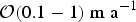
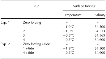
The design of the model geometry (see Fig. 1) is based on the ISOMIP Model 2 series of experiments (Hunter, Reference Hunter2006) with a modified geometry that is based on Grosfeld and others (Reference Grosfeld, Gerdes and Determann1997). A linearly sloping ice shelf covers the southern portion of the domain; it is 700 m at its deepest and 200 m at the ice front. The bathymetry is a constant 900 m depth. The horizontal grid resolution is ~10 km and the 24 vertical levels have a sigmoidal distribution, enhancing vertical resolution near both the upper and lower surfaces. For example, thicknesses of the upper, mid and lower cells are ~0.007, 0.078 and 0.02× the water column thickness, respectively. The model is initialised with a uniform temperature of −1.9°C and salinity of 34.4 (all salinities quoted are on the Practical Salinity Scale and are dimensionless). The model lateral boundaries are closed. The open ocean surface boundary is restored towards constant temperature and salinity values over a daily timescale, designed to create deep convection and develop a homogeneous water column. Cold cavity conditions are simulated by restoring the open ocean surface to −1.9°C and salinity of 34.5, while the hot cavity environment is simulated by relaxing the open ocean surface to 0.5°C and salinity of 34.6. The surface forcing conditions chosen for all model runs are approximately the same density.
Fig. 1. Model geometry from (a) side view, with bathymetry at 900 m below the surface and ice shelf shown in grey and every second sigma level shown in blue. (b) Ice shelf linearly slopes down to 700 m with a 200 m thick ice front at 76°S. Location of zones averaged for Fig. 3 are marked A and B.
Terrain-following vertical coordinate models, such as ROMS, are susceptible to pressure gradient errors where there are steep changes in water column thickness, for example at the ice shelf front. However, numerical algorithms employed in ROMS are designed to minimise the effect of pressure gradient errors (Shchepetkin and McWilliams, Reference Shchepetkin and McWilliams2003; Galton-Fenzi, Reference Galton-Fenzi2009). We have run a zero forcing test (results not shown) to determine the magnitude of pressure gradient errors; spurious currents are largest along the ice front, but are minimal (below 6 × 10⁻⁴ m s−1 for unstratified initial conditions) in comparison with the flow rate in the forced experiments. The change in ice thickness at the ice front occurs over one cell width, with a slope of ~1/50.
Ice shelf/ocean thermodynamics
Melting and freezing depends on the difference between the rate of ocean heat supplied to the ice/ocean interface, the rate of heat conducted into the ice shelf above and the in situ freezing point, which is modified by salinity and pressure. As the ocean flows past the ice interface, a boundary layer forms where the basal friction modifies the flow. The typical bottom boundary layer thickness is ${\rm \sim \!{\cal O}}(10)\;{\rm m}$
(Soulsby, Reference Soulsby and Johns1983), but will likely be somewhat different in the case of the ice/ocean boundary, due to the melting or freezing and the associated effects on stratification. Within the ice/ocean boundary layer (composed of an outer layer, log layer and viscous sublayer), velocity shear between the ice interface (at zero velocity) and the edge of the boundary layer (at the free-stream flow) generates turbulence. Heat and salt is then transported via turbulent exchange across the boundary layer, driving melting or freezing, which occurs at the thin liquid water layer adjacent to the interface (McDougall and others, Reference McDougall, Barker, Feistel and Galton-Fenzi2014). Modern numerical ocean models will typically have at least one cell in the boundary layer (the number will likely vary between models with different vertical coordinate systems and resolutions), and may or may not resolve the boundary layer/free-stream flow interface. Dynamics within the boundary layer, for example vertical turbulence-driven mixing of heat and salt, will not be resolved and hence must be parameterised.
${\rm \sim \!{\cal O}}(10)\;{\rm m}$
(Soulsby, Reference Soulsby and Johns1983), but will likely be somewhat different in the case of the ice/ocean boundary, due to the melting or freezing and the associated effects on stratification. Within the ice/ocean boundary layer (composed of an outer layer, log layer and viscous sublayer), velocity shear between the ice interface (at zero velocity) and the edge of the boundary layer (at the free-stream flow) generates turbulence. Heat and salt is then transported via turbulent exchange across the boundary layer, driving melting or freezing, which occurs at the thin liquid water layer adjacent to the interface (McDougall and others, Reference McDougall, Barker, Feistel and Galton-Fenzi2014). Modern numerical ocean models will typically have at least one cell in the boundary layer (the number will likely vary between models with different vertical coordinate systems and resolutions), and may or may not resolve the boundary layer/free-stream flow interface. Dynamics within the boundary layer, for example vertical turbulence-driven mixing of heat and salt, will not be resolved and hence must be parameterised.
Most current ice shelf/ocean models (e.g. Galton-Fenzi and others, Reference Galton-Fenzi, Hunter, Coleman, Marsland and Warner2012; Gladish and others, Reference Gladish, Holland, Holland and Price2012; Cougnon and others, Reference Cougnon, Galton-Fenzi, Meijers and Legrésy2013; Dansereau and others, Reference Dansereau, Heimbach and Losch2014; Gwyther and others, Reference Gwyther, Galton-Fenzi, Hunter and Roberts2014) simulate ice/ocean thermodynamic interaction using the three-equation parameterisation of Holland and Jenkins (Reference Holland and Jenkins1999), which assumes the ice shelf/ocean interface to be the local freezing point temperature. For more parameterisation details, see Holland and Jenkins (Reference Holland and Jenkins1999).
The heat flux across the boundary layer to the interface is given by $Q_{\rm M}^{\rm T} = {\rm \rho} _{\rm M} c_{{\rm p,M}} {\rm \gamma} _{\rm T} (T_{\rm B} - T_{\rm M} )$
, where ρM and c
p,M are the ocean density and heat capacity, respectively, and T
B and T
M are the temperatures at the ice shelf base and boundary layer, respectively. An analogous expression exists for
$Q_{\rm M}^{\rm T} = {\rm \rho} _{\rm M} c_{{\rm p,M}} {\rm \gamma} _{\rm T} (T_{\rm B} - T_{\rm M} )$
, where ρM and c
p,M are the ocean density and heat capacity, respectively, and T
B and T
M are the temperatures at the ice shelf base and boundary layer, respectively. An analogous expression exists for $Q_{\rm M}^{\rm S} $
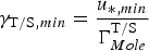
. Turbulent mixing to the ice/ocean interface is captured through turbulent exchange velocities,
$Q_{\rm M}^{\rm S} $
. Turbulent mixing to the ice/ocean interface is captured through turbulent exchange velocities,
 $$\gamma _{{\rm T/S}} = \displaystyle{{u_{\ast}} \over {\Gamma _{Turb} + \Gamma _{Mole}^{{\rm T/S}}}} $$
where T and S represent equations for heat and salt transfer respectively. The shear stress through the boundary layer, which creates turbulence, is described by the friction velocity, u
*. A quadratic drag formulation is commonly used to relate the friction velocity to the free-stream flow via a drag coefficient, C
D. Molecular diffusion through the thin, viscous sublayer ${\rm {\cal O}}(0.01)\;{\rm m}$
thick (Soulsby, Reference Soulsby and Johns1983) immediately adjacent to the ice interface is accounted for through
${\rm {\cal O}}(0.01)\;{\rm m}$
thick (Soulsby, Reference Soulsby and Johns1983) immediately adjacent to the ice interface is accounted for through $\Gamma _{Mole}^{{\rm T/S}} $
, while turbulent exchange across the boundary layer is parameterised with Γ
Turb
, following McPhee and others (Reference McPhee, Maykut and Morison1987) as,
$\Gamma _{Mole}^{{\rm T/S}} $
, while turbulent exchange across the boundary layer is parameterised with Γ
Turb
, following McPhee and others (Reference McPhee, Maykut and Morison1987) as,
 $$\Gamma _{Turb} = \displaystyle{1 \over \kappa} \ln \left( {\displaystyle{{u_{^\ast} \xi _{\rm N} {\rm \eta} _{^\ast}^2} \over {\,fh_{\rm \nu}}}} \right) + \displaystyle{1 \over {2\xi _{\rm N} {\rm \eta} _{^\ast}}} - \displaystyle{1 \over \kappa}, $$
where the von Kármán constant κ = 0.40, ξ N = 0.052 is a dimensionless stability constant, η* is the stability parameter (McPhee, Reference McPhee1981), h ν is the viscous sublayer thickness (Holland and Jenkins, Reference Holland and Jenkins1999) and f is the Coriolis parameter. We assume a destabilising buoyancy flux and set η* = 1, following others (Dansereau and others, Reference Dansereau, Heimbach and Losch2014). Since Γ Turb is undefined for u * = 0, we introduce a special condition as u * → 0, as discussed in section ‘Low-circulation limit’.
The turbulent exchange rates for heat and salt, γT/S, are often chosen to be velocity-independent, which assumes a non-realistic spatially and temporally constant flow rate past the ice/ocean interface. Including velocity-dependent turbulent exchange has been shown to improve accuracy of predicted melt rates in realistic geometry models, especially in the presence of strong currents and tides (e.g. Mueller and others, Reference Mueller2012; Dansereau and others, Reference Dansereau, Heimbach and Losch2014).
Low-circulation limit
The turbulent transfer coefficients introduced in the three-equation parameterisation (Holland and Jenkins, Reference Holland and Jenkins1999) were developed based on sea ice and laboratory studies (Kader and Yaglom, Reference Kader and Yaglom1972; McPhee and others, Reference McPhee, Maykut and Morison1987; McPhee, Reference McPhee1994). However, the sea ice/ocean interface is a different environment to the ice shelf/ocean interface, for example, the absence of wide-scale ice bottom slopes that lead to the strong buoyant plumes under ice shelves. The turbulent transfer coefficient scheme (McPhee and others, Reference McPhee, Maykut and Morison1987; Holland and Jenkins, Reference Holland and Jenkins1999) requires further investigation, for example, in the case of complex stratification (Kimura and others, Reference Kimura, Nicholls and Venables2015), for high vertical resolution models (Gwyther and others, Reference Gwyther, Galton-Fenzi, Dinniman, Roberts and Hunter2015), or for situations where a simpler parameterisation may suffice (Jenkins and others, Reference Jenkins, Nicholls and Corr2010). However, we wish to employ the melt parameterisation most often used by modellers, so as to make these results generally applicable or useful. As such, we apply a correction that accounts for the case of very weak flow with negligible turbulence.
The implementation of a lower limit on u
* in the three-equation parameterisation is necessary to ensure the melt rate does not become undefined. The turbulent transfer coefficient (Γ
Turb
; Eqn (2)) contains the natural logarithm of u
*, which is undefined for stationary water. (Note: Γ
Turb
is also undefined for f = 0, i.e. at the equator.) (u
* = 0), and approaches negative infinity as u
* → 0. It follows that the calculation of γT/S must be implemented with a conditional statement to set the turbulent transfer coefficient to zero if boundary layer flow reaches a minimum threshold, u
*,min
. This is achieved by setting Γ
turb
= 0 and enforcing u
* = u
*,min
, in which case Eqn (1) will simplify to ${\rm \gamma} _{{\rm T/S},min} = \displaystyle{{u_{*,min}} \over {\Gamma _{Mole}^{{\rm T/S}}}} $
.
${\rm \gamma} _{{\rm T/S},min} = \displaystyle{{u_{*,min}} \over {\Gamma _{Mole}^{{\rm T/S}}}} $
.
The justification for implementing a minimum friction velocity is the case where flow along the ice/ocean interface is laminar, and heat transfer can occur through diffusion alone. The rate of heat transfer across the unresolved portion of the log layer (from the centre of the top model cell to the interface) will result only from the molecular diffusion of heat in seawater (κ T = 1.4 × 10⁻⁷ m s−1). From Eqns (1) and (2), a value of u *,min = 2 × 10⁻⁵ m s−1 leads to γT/S,min being approximately equivalent to heat transfer by molecular thermal diffusion (κ T), to within an order of magnitude.
In reality, the presence of tidal currents will likely ensure currents are larger than the u *,min limit. However, at the shallow water column near grounding zones (Holland, Reference Holland2008) or at slack water, tidal currents may be weak enough that they fall below the u *,min limit; in these cases it is necessary to ensure that a lower limit is placed on u *. Furthermore, the definition of u *,min presented here may also be relevant for sea ice models.
Experimental design
Experiment 1: melt relationship with cavity temperature
This experiment investigates the changes in melt rate distribution and magnitude for four different thermal environments, from a cold to hot ocean cavity. For each run, the surface forcing is achieved by restoring the open ocean surface to a different set of salinity and temperature values (see Table 1) on a daily timescale. All simulations are run for 30 years, at which point they are in a pseudo steady state. A zero forcing run (no surface or lateral forcing, tides or ice shelf thermodynamics and unstratified ocean conditions) is conducted to test for spurious flow resulting from pressure gradient errors.
Table 1. Summary of experiments showing the surface forcing conditions that drive variation in oceanic environment
Experiment 2: tidal forcing
In a cold cavity environment, we expect low thermal driving will decrease melting and buoyant circulation and as a result circulation within the ice shelf cavity will be weak, as shown by many modelling studies (e.g. Holland and others, Reference Holland, Jacobs and Jenkins2003). However, as mentioned previously, it is likely that tidal currents are important for maintaining a significant background flow and will change the circulation within the cavity (Makinson and others, Reference Makinson, Holland, Jenkins, Nicholls and Holland2011; Mueller and others, Reference Mueller2012; Arzeno and others, Reference Arzeno2014). This study investigates how circulation and melting in a hot and cold ocean cavity are altered by the addition of a simple analogue of tides. Furthermore, we assess the friction velocity generated by tides in the absence of buoyancy-driven circulation by removing ice shelf thermodynamics and surface forcing (zero forcing + tide, Table 1).
There are several possibilities for incorporating the influence of tides. A common approach is to set constant turbulent exchange coefficients, ΓT/S, chosen such that they parameterise a constant background current representative of tidal flow (see Losch, Reference Losch2008). However, this will not allow spatial or temporal variation in turbulent exchanges due to buoyancy-driven flow or tidal variability. Another option is to add an offset in the calculation of the friction velocity, equivalent to a root-mean-square (RMS) tidal current. For example, by modifying the velocity u used in the calculation of u *, u = u′ + |u| tide , where u′ is the velocity without tides, and |u| tide is the constant value equal to the RMS tidal current. The offset will impose a lower threshold on currents, equivalent to the mean tidal flow (as suggested by Jenkins and others, Reference Jenkins, Nicholls and Corr2010). However, this approach does not capture other effects associated with tides, such as internal tides horizontal mixing and vertical shear driven mixing. We directly include tides by clamping the north-south vertically-integrated velocity on the northern boundary to be a sinusoid with amplitude 0.1 m s–1, and period of 12.00 h. This approach generates an idealised tidal wave with period exactly equivalent to the principal solar constituent (S 2). The critical latitude (where the tidal frequency equals the Coriolis or inertial frequency) for this modified S 2 tide is ~85.8°S, which is well south of the southern boundary of the model domain and therefore unlikely to cause more complex tidal dynamics as have been found in ice shelf cavities where the critical latitude is closer to the ice shelf (e.g. Makinson and others, Reference Makinson, Schröder and Østerhus2006; Robertson, Reference Robertson2013). The boundary remains closed to temperature and salinity, as in Experiment 1, and the surface forcing is identical to the respective run of Experiment 1 (see Table 1). Note that the model surface (including under the ice shelf) is free to move up and down. This approach will allow for tidal mixing by friction with the basal and bathymetric surfaces, as well as allow for spatial and temporal variation in turbulent exchange, and has been employed by various realistic applications (e.g. Galton-Fenzi and others, Reference Galton-Fenzi, Hunter, Coleman, Marsland and Warner2012; Mueller and others, Reference Mueller2012).
The time step and output frequency were chosen to be multiples of the tidal period to minimise tidal aliasing. The model is spun up for 29 years, and analysis is conducted on the temporal average of the 30th year of model output.
RESULTS
Experiment 1: melt relationship with cavity temperature
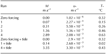
Between run 1 and run 4, the area-averaged melt rate increases ~41×, the area-averaged u * increases ~9× and the area-averaged T * increases ~4× (see Table 2). In line with Holland and others (Reference Holland, Jenkins and Holland2008) we find a quadratic increase in melt as the oceanic temperature is increased, resulting from the combined linear increases in friction velocity and thermal driving as ocean temperature is increased; melting increases approximately linearly with u * T * (slope of 7× 10⁻⁵°C−1). More data points would need to be added to confirm this quadratic trend.
Table 2. Summary of area averaged melt rate, friction velocity and thermal driving for each experiment
The spatial distribution of steady-state melting (positive) and freezing (negative) is shown in the first column of Figure 2. The location of highest melt moves eastward as the cavity environment is warmed. Likewise, melting along the ice front is stronger for the warmer cavities. For runs 2–4, melting and freezing at the northwest of the ice shelf displays some grid-scale noise; this is also seen in Losch (Reference Losch2008).
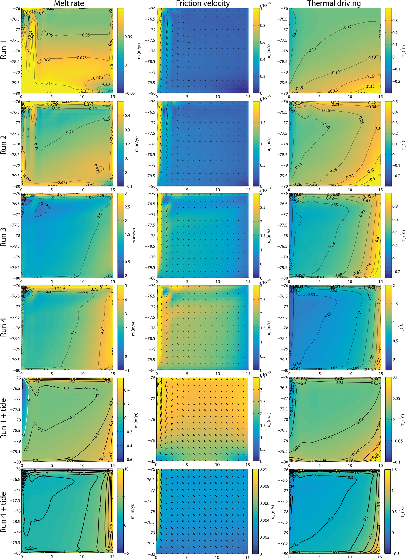
Fig. 2. Temporally-averaged melt rate (melting for m > 0; column 1), friction velocity (column 2) and thermal driving (column 3) are shown for each model run. Vectors in the friction velocity plot represent the temporally-averaged flow direction (every fourth grid cell) and are scaled to the maximum magnitude of u * for each plot. Run 1 represents the coldest conditions, and run 4 the warmest conditions. The fifth row (run 1 + tide) is identical to run 1 except for the addition of an analytic tide on the northern boundary. The sixth row (run 4 + tide) is identical to run 4 except for the addition of an analytic tide on the northern boundary. Note the changes in colour scale between some plots.
The spatial variation in melting for different cavity environments is further investigated with melt rate transects shown in Figure 1. These transects are calculated as the melt rate along each line of longitude/latitude within the bounds of the area A/B, as a proportion of the average melt rate over the total area of A/B. For the cold cavity, melting is strongest at the southern and western ends of the cavity. As the cavity warms, melting at the western edge (Fig. 3a) and in the southern half (Fig. 3b) of the cavity decreases relative to the mean, while melting along the eastern edge and close to the ice front increases relative to the mean.
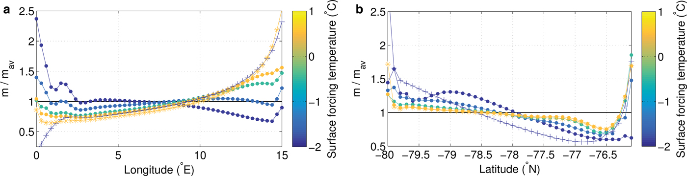
Fig. 3. (a) Melt/freeze rate along transect A as a proportion of the area averaged melt rate for the same transect. Melting along the transect is calculated as the meridional average within the area of A (see Fig. 1) for each point along the transect. (b) Melt/freeze rate along transect B as a proportion of the area averaged melt rate for the same transect. Melting along the transect is calculated as the zonal average within the area of B (see Fig. 1) for each point along the transect. Transects are coloured for the temperature of surface forcing. Runs 1–4 are represented with solid dots, while run 1 + tide is represented with + and run 4 + tide is represented with *. The horizontal black line at m/m av = 1 represents where melting along the transect is equal to the transect-average melt rate.
The friction velocity, u
*, is shown in the second column of Figure 2, and is calculated as the top layer speed multiplied by $\sqrt {C_{\rm D}} $
. In general, cavity circulation in the top model cells is from east to west, with strong acceleration as the flow intercepts the western boundary. At the western boundary, flow turns and increases to the north. As the cavity temperature increases, the magnitude of flow increases. Several interesting features appear: Stronger flow adjacent to the ice shelf front; and, a southward deviation in flow before flowing north along the western boundary (at approximately the 1.5°E meridian). The ice front jet is possibly formed by buoyancy-driven circulation exiting the cavity, combined with the meltwater formed by strong melting at the ice front. The southwards flow along the 1.5°E meridian is in response to the deep outflow plume that extends to the cavity floor: volume conservation drives weak inflow seen along the 1.5°E meridian; this is very similar to the clockwise-rotating gyre seen in Losch (Reference Losch2008). The 76.5°S zone has currents that fluctuate northwards to southwards as a result of influence from the meandering ice front jet. As a result, the time averaged u
* is lower.
$\sqrt {C_{\rm D}} $
. In general, cavity circulation in the top model cells is from east to west, with strong acceleration as the flow intercepts the western boundary. At the western boundary, flow turns and increases to the north. As the cavity temperature increases, the magnitude of flow increases. Several interesting features appear: Stronger flow adjacent to the ice shelf front; and, a southward deviation in flow before flowing north along the western boundary (at approximately the 1.5°E meridian). The ice front jet is possibly formed by buoyancy-driven circulation exiting the cavity, combined with the meltwater formed by strong melting at the ice front. The southwards flow along the 1.5°E meridian is in response to the deep outflow plume that extends to the cavity floor: volume conservation drives weak inflow seen along the 1.5°E meridian; this is very similar to the clockwise-rotating gyre seen in Losch (Reference Losch2008). The 76.5°S zone has currents that fluctuate northwards to southwards as a result of influence from the meandering ice front jet. As a result, the time averaged u
* is lower.
The thermal driving, T *, shown in the third column of Figure 2, is calculated as the difference between the in situ temperature and the in situ (pressure-dependent) freezing point. The magnitude of T * increases with the temperature of the cavity, and the thermal gradient in T * rotates counterclockwise as the cavity temperature is increased. The increased thermal driving present on the eastern boundary is the result of stronger overturning circulation delivering hotter cavity water to the ice shelf base.
The column averaged potential temperature increases as expected between run 1 and run 4 (Fig. 4), while the zonal average temperature shows a colder boundary layer region in the hotter cavity (Fig. 5). The warmer surface forcing conditions produce warmer water both in the open ocean (to the full depth of the model) and within the cavity. The barotropic and overturning streamfunction, shown as contours in Figures 4 and 5, respectively, are stronger in the hot cavity run than for the cold cavity run. Patterns of circulation for both cavity environments are similar; the barotropic streamfunction is clockwise within the cavity, while the overturning circulation is up the ice shelf slope and downwards in the open ocean. The increased circulation between run 1 and run 4 leads to divergent upwelling, which can be seen as the band of higher column average temperature along the southern and eastern boundary in run 4 (Fig. 4). The column averaged salinity has almost identical distribution to the column average potential temperature and therefore is not shown.
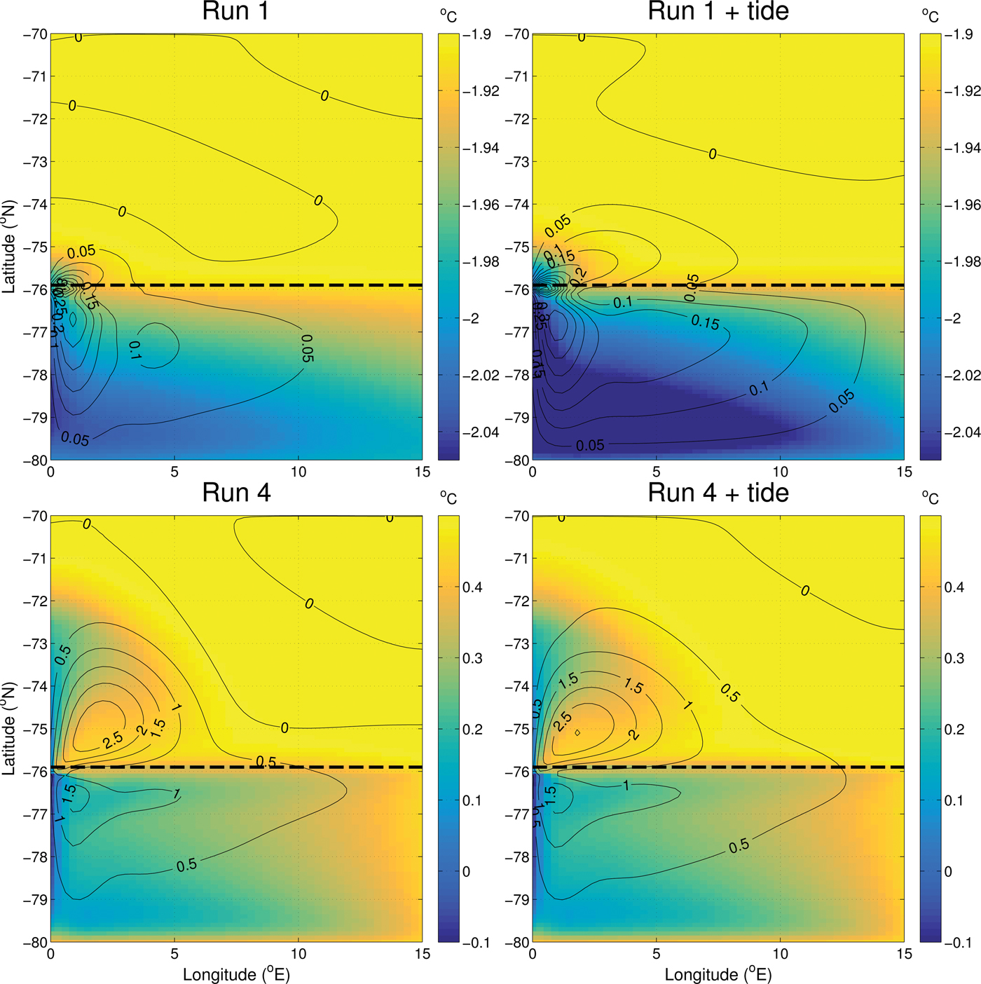
Fig. 4. Column averaged potential temperature, with contours showing the barotropic streamfunction for runs 1, 4, 1 + tide and run 4 + tide. Note the different colour scales between the cold and hot cavity model runs. Contours have units of Sverdrups and positive circulation is defined as clockwise.
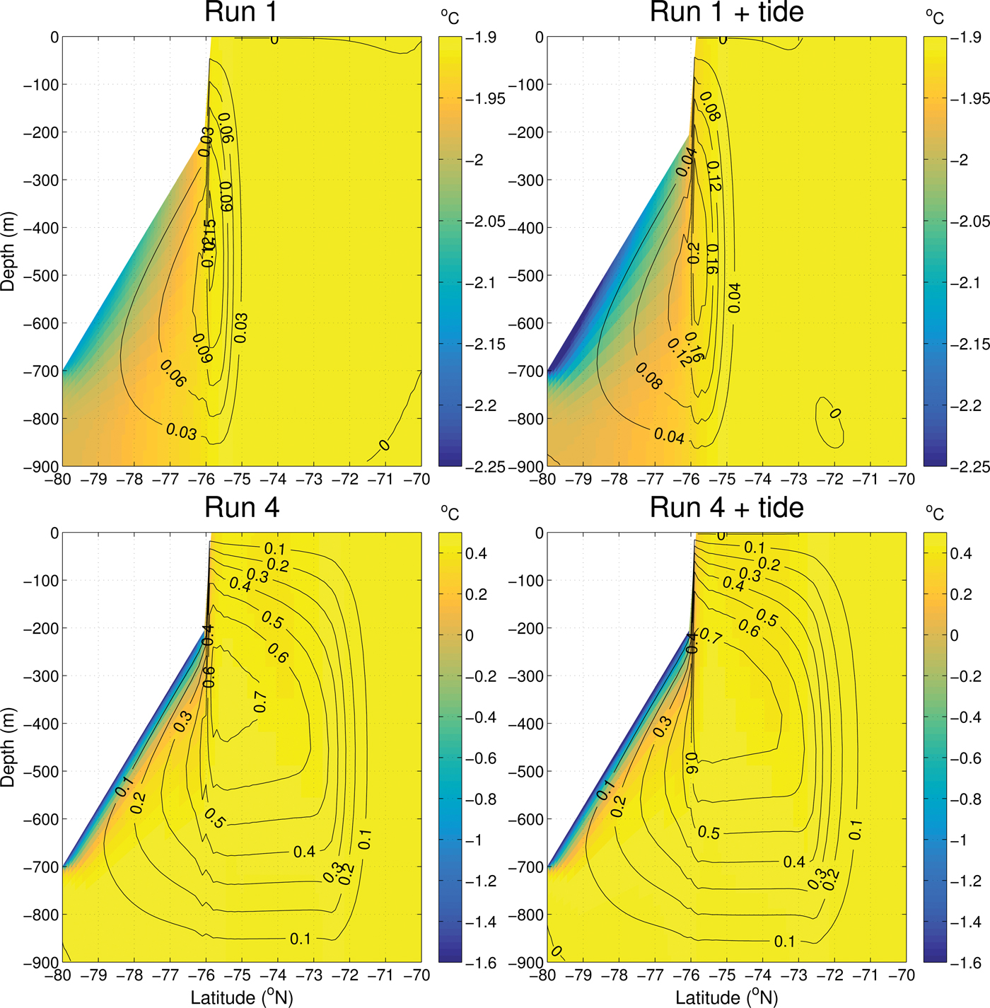
Fig. 5. Zonal average potential temperature, with contours showing the overturning streamfunction for runs 1, 4, 1 + tide and run 4 + tide. Note the different colour scales between the cold and hot cavity model runs. Contours have units of Sverdrups and positive circulation is defined as clockwise.
Experiment 2: tidal forcing
To investigate the impact that tides have on circulation, separate from the buoyancy-driven circulation, we have run a simulation with tides but without ice/ocean thermodynamics (zero forcing + tide; Table 1). The results of this simulation show how tidal currents are distributed. The magnitude of depth-averaged tidal currents (|u| tide ) is shown in Figure 6. Strongest tidal currents exist across the front half of the shelf (76°S to 78°S), and at the northwest and northeast boundaries. The southern region of the ice shelf experiences weakest tidal currents, with the southwest and southeast corners of the ice shelf experiencing almost negligible flow. The effective friction velocity is u *,tide = 3 × 10⁻³ m s−1, as calculated from the area-average |u| tide (see Table 1).
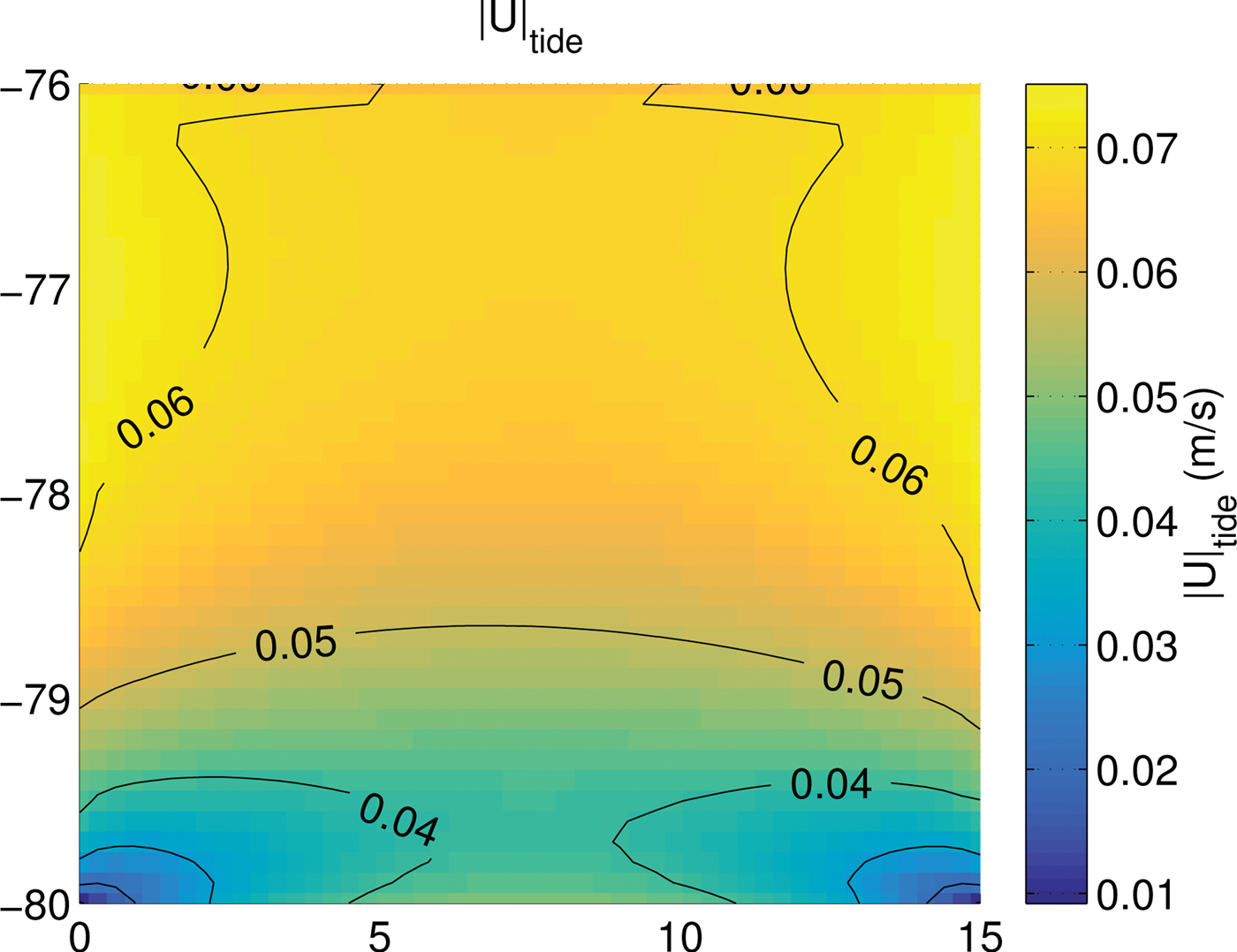
Fig. 6. The depth-averaged RMS tidal velocity for the zero forcing + tide run, showing strongest currents across the middle of the ice shelf. The currents are temporally-averaged across an integer number of tidal cycles.
The effects of idealised tidal forcing on the temporally averaged melt rate, friction velocity and thermal driving for the forced models are shown in the fifth and sixth rows of Figure 2. Distribution and magnitude of melting are dramatically altered, compared with the simulation with the same thermal forcing but without tidal forcing (compare run 1 against run 1 + tide and run 4 against run 4 + tide); melting is strong (m ~ 0.5 m a−1 for the cold cavity, m ~ 1.5 m a−1 for the hot cavity) at the deep grounding line in the southeast corner of the ice shelf and decreases in magnitude moving northwest. Melting is also strengthened along the ice shelf front. A significant patch of refreezing now forms along the western boundary of run 1 + tide. Compared with the run without tides, melting is below average in the southwest and above average in the southeast for both cold and hot cavities (Fig. 3a). The north-south transect in melting for the cold cavity displays stronger than average melting adjacent to the ice shelf front and towards the grounding line, compared to the run without tides (Fig. 3b). The proportional change in melting along the north-south transect for the hot cavity run when tides are added is very small.
Between run 1 + tide and run 4 + tide, the area-averaged melt rate increases ~24×, the area-averaged u * increases ~1.2× and the area-averaged T * increases ~22× (see Table 2). The run 1 + tide and run 4 + tide data, fit with a linear relationship given by m tide = α tide u *,tide T *,tide , has a slope of α tide = 7.5 × 10⁻⁵°C−1. This slope is marginally larger than for without tides. Given that only two data points are used for this regression, we cannot conclude that this slope is the same as that for the runs without tides (as would be expected), or if it is indicative of nonlinear dynamics within the ocean acting to increase u * or T *. There is also a larger relative increase in melting for the cold cavity (2× as much melting) than for the hot cavity (1.2× as much melting) when tides are included. The temporal evolution of velocity and melting (not shown) displays an exact proportionality between strong tidal flow and high melting.
The magnitude of friction velocity when tides are included is increased for the entire domain, except towards the grounding line with minima located in the southwest and southeast corners of the ice shelf.
For both the experiments, the thermal driving is reduced across the entire ice shelf, compared with the runs without tides. The maximum of T * still occurs in the southeast corner of the ice shelf, while the region along the western boundary, which displays negative T * in run 1 + tide is now increased in areal extent and magnitude.
The addition of tides leads to a colder column averaged temperature (Fig. 4), through increased meltwater discharge. A band of colder water is noticeable in the southwest of run 1 + tide. This results from the tidal currents driving stronger melting, and releasing cold meltwater, which flows westwards and then northwards along the western boundary. The colder meltwater plume is also noticeable in the zonal average temperature (Fig. 5). The overturning and barotropic streamfunctions increase in magnitude when tides are added.
DISCUSSION
Buoyant convection (resulting from the chosen surface forcing) delivers heat and salt to the bottom layers of the model, which are then advected to the base of the ice shelf. Strong stratification is only present within the meltwater plume, which is seen to rapidly mix into the open ocean via surface-flux driven convection. Tides have a minimal impact on the open ocean temperature and salinity, as mixing from the buoyant convection is already effective at homogenising the open ocean conditions. The barotropic streamfunction shows broad inflow into the cavity on the eastern side and a western boundary current outflow, similar to that shown by Losch (Reference Losch2008). The inflow into the east of the hot cavity is strong (between 0.25 and 0.5 Sv) and delivers the hot water to drive melting in this region. For all but the coldest cavity environments, melting along the ice shelf front is strong. The high thermal driving results from the presence of hot open ocean water at the ice front, which together with the presence of the ice front jet produces strong melting. The ice front jet is driven by circulation deflecting under the influence of the Coriolis effect combined with baroclinic flow resulting from the addition of fresh meltwater at the ice front. However, it is unclear how much the numerical issues associated with the vertical discretisation contribute to the formation of this jet, and so further investigation is warranted. Strong flow along the front of ice shelves have been observed (e.g. Ross Ice Shelf; Keys and others, Reference Keys, Jacobs and Barnett1990) and also shown in other models (e.g. Makinson and others, Reference Makinson, Holland, Jenkins, Nicholls and Holland2011; Mueller and others, Reference Mueller2012), but it is not certain if the same mechanisms are at play here.
The distribution of melting over the rest of the ice shelf changes as the cavity temperature warms: maximum melting shifts from the western boundary to the eastern boundary (compare runs 1 and 4 in Fig. 2). This is due to the increasing influence of the warmer oceanic waters driving stronger melting. In the cold cavity, the meltwater plume is weak, leading to limited upwelling at the eastern boundary due to divergent flow. Limited upwelling results in T * being small, however at depth, there is enough heat relative to the in situ freezing point to cause melting and removal of heat from the ocean; closer to the ice front the cold meltwater ascending from depth leads to refreezing. In the hot cavity, the strong westwards meltwater flow introduces warm sub-cavity water to the ice base via divergent flow at the eastern boundary. The stronger supply of warmer water drives greater melting at the eastern boundary relative to the cold cavity. The increased buoyant meltwater production and circulation forms a positive feedback on melting. However, In the presence of tidal currents, the change in melt between cold and hot cavities is less noticeable. For present day steady-state melting of ice shelves, we therefore expect different patterns of melting and locations of strongest melt, depending on the cavity environment.
In general, these results suggest that increasing the temperature of the ocean cavity environment will lead to a shift in the melt pattern. As the ocean temperature increases, melting and buoyant meltwater production increases, resulting in stronger circulation and therefore u *, driving a feedback which further enhances the supply of warm water to the ice shelf base. Melting shifts from the western to the eastern boundary as the wide-scale circulation becomes dominated by buoyancy-driven flow. As the circulation increases, there is a concurrent change in the amount of heat available to drive melting; increased circulation supplies more warm water to the ice shelf base, and release cold meltwater, which flows to the western boundary. Both effects combine to move the pattern of strongest melting from the western boundary to the eastern boundary as the cavity environment is warmed. For example, an ice shelf with a similar cavity environment to run 4 + tide (e.g. Pine Island Ice Shelf) that undergoes ocean warming, might experience only a small shift in the distribution of melting, as compared with a cold cavity ice shelf undergoing the same warming.
The faster currents that result from the tidal forcing act to increase melting. However, increased meltwater production and stronger tidal mixing cools the boundary layer and reduces thermal driving, as compared with the simulation without tides (Fig. 2). Melting at the ice front results from strong flow across and along the ice front combined with the proximity to the warm open ocean water. The increased production of meltwater results in stronger refreezing over a larger area for the cold cavity; indeed, the changes to the distribution of melting due to inclusion of tides is largest when the thermal environment of the cavity is cold. Barotropic tidal velocities go to zero at the corners, through both the standard response of flow at a corner, and increasing friction from the ice and bottom surfaces as the water column thins. Strong tidal currents near the ice front and weak tidal currents near the grounding line have also been shown in realistic simulations (Mueller and others, Reference Mueller2012). The effect on basal melting of including tides in idealised experiments is shown to be substantial, in agreement with realistic simulations (e.g. Galton-Fenzi, Reference Galton-Fenzi2009; Makinson and others, Reference Makinson, Holland, Jenkins, Nicholls and Holland2011; Mueller and others, Reference Mueller2012; Robertson, Reference Robertson2013; Arzeno and others, Reference Arzeno2014). These effects may change depending on how realistic geometry affects tidal currents. For example, in the thin water column near the grounding zone, a tidal front may protect the ice from inflowing oceanic heat and lead to reduced melting (Holland, Reference Holland2008). This does not occur in our simulations, as the water column thickness at the southern boundary is too great (200 m).
Previous idealised studies have shown an increase in melt as the ocean temperature is increased (Holland and others, Reference Holland2008; Goldberg and others, Reference Goldberg2012). However, the model architecture (isopycnal coordinates) of these studies differs from ROMS (terrain-following vertical coordinate). As such, the similar response of melting to increasing ocean temperature between these previous studies and this study is reassuring. Yet, spatial melt magnitude and distribution for cold and hot scenarios, as presented here, show some differences to other studies. The melt distribution in the cold cavity features a maximum along the outflow boundary. Losch (Reference Losch2008) did not show this distribution, potentially as a result of the velocity-dependent melt formulation chosen in this current study. The values of γT/S chosen in Losch (Reference Losch2008), with γT = 1 × 10⁻⁴ and γS = 5.05 × 10⁻⁷, are equivalent to an effective u * ≈ 9 × 10⁻³ m s−1. The magnitude of u * implicit in Losch (Reference Losch2008) is equivalent to very strong RMS tidal forcing (high compared with the effective u * simulated here: u *,tide = 3 × 10⁻³ m s−1; Table 2). The strong implicit RMS tidal forcing also explains why the melt distribution of Losch (Reference Losch2008) is similar to run 1 + tides in this study. This is because the temporal-average of our idealised tidal forcing is similar to increasing the mean circulation by the RMS tidal current, which in Losch (Reference Losch2008) is implicit by assuming constant exchange rates. Holland and others (Reference Holland, Jenkins and Holland2008) showed a similar location of maximum melt, which did however not extend further north along the outflow boundary. The reasons for this difference are unclear, but could be related to the different model framework. In the hot cavity, melting is strong in a narrow band along the inflow boundary, unlike in Dansereau and others (Reference Dansereau, Heimbach and Losch2014) where melting is strongest along the outflow boundary. This difference can be explained as a result of the velocity field responding to the strong inflow currents, which are a feature of the lateral boundary conditions chosen in Dansereau and others (Reference Dansereau, Heimbach and Losch2014). In this study, there is no forced inflow, and as a result the sub-ice velocity field is due to buoyancy-driven circulation.
This study shows a general distribution of melting for different cavity environments; maximum melting in a cold ice shelf cavity is likely to be distributed near to the outflow region, while in a hot cavity will be distributed nearer to the inflow. This result can be applied to an ice shelf, which is transitioning from a cold cavity to a hot cavity under the influence of warmer ocean conditions; melting will shift to a maximum near to the eastern side of the cavity. Our results suggest that an increase in ocean temperature by 2.4°C will increase melting by ~24× (~41× excluding tides); as an example, the total area-averaged melt rate for all ice shelves is 0.94 m a−1 (Depoorter and others, Reference Depoorter2013), which under 2.4°C of warming would increase to 22 m a−1. Realistic simulations of the cold to hot cavity transition of Filchner-Ronne Ice Shelf (due to a 2°C warming) found a change in area average melt from 0.2 to 4 m a−1, a 20× increase (Hellmer and others, Reference Hellmer, Kauker, Timmermann, Determann and Rae2012). While we urge caution in using results of an idealised simulation (with an accompanying idealised geometry and forcing scenario) to make realistic projections, we highlight the similarity of our results to the realistic simulation of Filchner-Ronne Ice Shelf. Like Hellmer and others (Reference Hellmer, Kauker, Timmermann, Determann and Rae2012), our results (0.2 m a–1 increasing to 4.8 m a–1) suggest that an ice shelf that undergoes a transition from cold to hot cavity conditions will experience a large increase in mass loss, leading to decreased buttressing and the retreat of tributary glaciers.
CONCLUSIONS
We use an adapted version of ROMS with the three-equation parameterisation, velocity-dependent turbulent exchange, and the KPP of vertical mixing to conduct idealised simulations of ice shelf/ocean interaction. These idealised simulations investigate the effect on melt distribution and magnitude as the cavity environment is altered.
Melting is driven by the availability of heat and the flow speed near the ice interface. However, this study suggests that a cold cavity ice shelf that undergoes a transition to a hot cavity will experience a change in the location of strongest melting. For example, in the absence of significant tides, buoyancy-driven circulation in a cold cavity environment is weak and there is minimal upwelling of heat, leading to weaker melting focused on the western outflow. As the cavity temperature is increased, buoyancy-driven circulation becomes stronger than the outflow current. Together with the increased upwelling of warmer water, this leads to increased melting located most strongly where the upwelling is occurring – at the eastern boundary. When significant tides are present, the pattern of basal melting still shifts although not as dramatically. We conclude that the pattern of melting will shift as the cavity temperature is increased. Warming ocean conditions will change melt distribution more for cold cavity ice shelves as compared with hot cavity ice shelves.
Idealised tidal forcing acts to increase barotropic and overturning circulation strength and hence melting. The increased meltwater production decreases thermal driving, but not enough to lower melting. Adding tidal forcing to an ice shelf/ocean model drives stronger currents across the front half of the ice shelf area and leads to an increase and redistribution in melting. However, the effect of tidal forcing on the relative increase in melt rate is greatest for a cold ocean cavity environment. These results further justify the inclusion of velocity-dependent turbulent exchange and tides in the application of an ice shelf/ocean model to a realistic domain.
The change in the magnitude and distribution of melting with the cavity thermal environment has implications in possible future warming scenarios. By warming the ocean cavity by 2.4°C, melting increased by ~24× when including tides (~41× without tides) and the distribution of melting shifted to the eastern side of the cavity. These experiments used idealised geometry and forcing conditions, and so must be understood in this context.
ACKNOWLEDGEMENTS
The authors acknowledge and thank Dr Laurie Padman and an anonymous reviewer as well as editors Dr Christopher Little and Dr Tony Payne for critique and suggestions. This work was supported through the Australian Government's Cooperative Research Centre Programme through the Antarctic Climate & Ecosystems Cooperative Research Centre and through the Australian Research Council's Special Research Initiative for Antarctic Gateway Partnership (Project ID SR140300001). David Gwyther was supported by the Australian Government CSIRO and University of Tasmania through the Quantitative Marine Science PhD program. Computing resources were provided by both the Tasmanian Partnership for Advanced Computing and the National Computational Infrastructure under grant m68.


 Open access