
Implications
The Global Livestock Environmental Assessment Model (GLEAM) is intended to provide a level of analysis that has sufficient technical rigour, but can also be translated into practical advice to decision-makers (e.g. governments, project planners, producers, industry and civil society organizations). It is hoped that its features, such as the ability to derive rations for livestock in developing countries, and to capture variation in livestock performance and management, will support improvement of the environmental performance of livestock production.
Introduction
The livestock sector is one of the fastest growing subsectors of the agricultural economy. Demand for all the main livestock commodities are forecast to increase significantly between now and 2050 (see Alexandratos and Bruinsma, Reference Alexandratos and Bruinsma2012). Although the livestock sector makes an important contribution to global food supply and economic development, it also uses significant amounts of natural resources and impacts on the environment (see e.g. Steinfeld et al., Reference Steinfeld, Gerber, Wassenaar, Castel, Rosales and de Haan2006; Herrero and Thornton, Reference Herrero and Thornton2013; Leip et al., 2015). One of the most important global impacts arises from the emission of greenhouse gases (GHG) along livestock supply chains, which are estimated to make a significant contribution to overall anthropogenic GHG emissions (Gerber et al., Reference Gerber, Steinfeld, Henderson, Mottet, Opio, Dijkman, Falcucci and Tempio2013).
If the GHG emissions intensities (Ei) (i.e. the kg of GHG per kg of animal product) of livestock commodities are not reduced, the forecast increases in production will lead to proportionate increases in GHG emissions, compromising efforts towards climate change mitigation. It is therefore essential that ways are found to improve efficiency and reduce the Ei of livestock production (while noting that such supply-side improvements may be complemented by measures to reduce demand, Bajželj et al., Reference Bajželj, Richards, Allwood, Smith, Dennis, Curmi and Gilligan2014; Lamb et al., Reference Lamb, Green, Bateman, Broadmeadow, Bruce, Burney, Carey, Chadwick, Crane, Field, Goulding, Griffiths, Hastings, Kasoar, Kindred, Phalan, Pickett, Smith, Wall, zu Ermgassen and Balmford2016). Improving our understanding of where and why emissions arise in livestock supply chains is an important step towards achieving this goal.
In order to improve our understanding of livestock’s environmental impact, the Food and Agriculture Organization of the United Nations (FAO) has developed GLEAM (http://www.fao.org/gleam/en/). The primary motivation behind GLEAM was the desire to have a tool that enabled comprehensive, disaggregated and consistent analysis of the environmental performance of global livestock production to support the identification of improvement options. This is important as methodological inconsistencies between studies can make it difficult to determine whether apparent differences in results arise from differences in actual emissions or in methodologies, thereby complicating the identification of mitigation options.
The global GHG emissions produced by livestock have been quantified in the assessment reports for the United Nations Framework Convention on Climate Change (Smith et al., Reference Smith, Bustamante, Ahammad, Clark, Dong, Elsiddig, Haberl, Harper, House, Jafari, Masera, Mbow, Ravindranath, Rice, Robledo Abad, Romanovskaya, Sperling and Tubiello2007 and Reference Smith, Martino, Cai, Gwary, Janzen, Kumar, McCarl, Ogle, O’Mara, Rice, Scholes and Sirotenko2014). In addition, there are several databases of global emissions, such as: US Environmental Protection Agency Global Emissions Database (EPA, 2012); European Commission Joint Research Centre’s Emissions Database for Global Atmospheric Research (EDGAR, 2012); the World Resource Institute’s CAIT (Climate Analysis Indicators Tool) (WRI, 2013); and the FAOSTAT online database of agricultural GHG emissions (Tubiello et al., Reference Tubiello, Salvatore, Rossi, Ferrara, Fitton and Smith2013). These analyses predominantly adopt IPCC (2006) Tier-1-type approaches to the quantification of livestock emissions and focus on the emissions produced in one part of the supply chain, that is on-farm. The Global Livestock Environmental Assessment Model seeks to complement and add value to these analyses by using a herd model coupled with an IPCC (2006) Tier 2 approach to computing emissions, thereby enabling key characteristics of the livestock populations (e.g. herd structures, animal performance, rations and manure management) to be captured in the calculations. Further, GLEAM adopts a life-cycle approach and calculates the emissions arising along the supply chain from cradle to retail point. This enables the Ei of specific commodities to be calculated rather than just the total emissions from an agricultural subsector. Finally the reliance on geographical information systems (GIS) provides spatially explicit analysis and flexibility in combining data sets and aggregating results.
Initial development of GLEAM has focussed on the GHG element, as FAO is committed to supporting member countries and stakeholders in the livestock sector to identify low-emission development pathways for animal production. The development of GLEAM is one part of continuing efforts by FAO to improve assessment of the sector’s GHG emissions. Three technical reports present the results of the global analysis undertaken with GLEAM to date for (a) the cattle dairy sector (Gerber et al., Reference Gerber, Opio, Vellinga, Henderson and Steinfeld2010); (b) the pig and chicken sectors (MacLeod et al., Reference MacLeod, Gerber, Vellinga, Opio, Falcucci, Tempio, Henderson, Mottet and Steinfeld2013); (c) the cattle, buffalo and small ruminant sectors (Opio et al., Reference Opio, Gerber, Vellinga, MacLeod, Falcucci, Henderson, Mottet, Tempio and Steinfeld2013). A fourth report provides a synthesis of the three technical reports and identifies options to reduce emissions (Gerber et al., Reference Gerber, Steinfeld, Henderson, Mottet, Opio, Dijkman, Falcucci and Tempio2013).
The purpose of this paper is to provide a review of GLEAM. Specifically, it presents an overview of the model architecture, methods and functionality. It then briefly compares GLEAM results with other studies and explains how differences can arise. In the last section, the advantages of GLEAM are discussed, along with challenges and priorities for development. The Global Livestock Environmental Assessment Model is undergoing continuous development, so any review can only provide a snapshot of the model at a given time. This review focuses on GLEAM version 1.0 (which was used to undertake the analysis for the reports cited in the previous paragraph), while highlighting some revisions introduced in version 2.0, and referring to the most up to date model description (FAO, 2017).
Overview of the Global Livestock Environmental Assessment Model architecture, methods and functionality
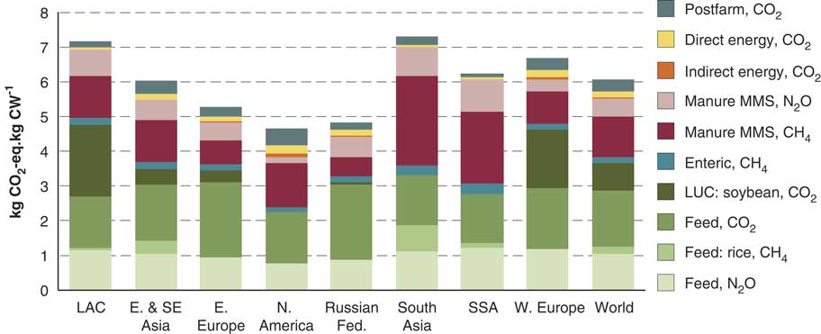
The Global Livestock Environmental Assessment Model includes the main livestock production activities and quantifies the related GHG emissions. It includes the following activities along the supply chain: (a) pre-farm emissions arising from the manufacture of inputs; (b) on-farm emissions during feed and animal production; and (c) post-farm emissions arising from the processing and transportation of products to the retail point. The GHG emissions included in GLEAM v1.0 are summarized in Table 1. The model differentiates 11 main global livestock commodities, which are: meat and milk from cattle, sheep, goats and buffalo; meat from pigs; and meat and eggs from chickens. It also distinguishes between the main production systems, for example three distinct pig systems are defined which differ in terms of their herd parameters, rations, excretion rates, manure management etc. (see FAO, 2017, section 1.5 for details of the production system classification used). It calculates the GHG emissions and commodity production for a given system within a grid of spatially defined cells, thereby enabling the calculation of the Ei for any desired combinations of commodities, farm systems and locations at different spatial scales. An example of GLEAM output is given in Figure 1.

Figure 1 Regional average emission intensity of pig meat production from all three systems (regions with <1% of total production are omitted). LAC=Latin America and Caribbean; SSA=Sub-Saharan Africa; Manure MMS=emissions arising from manure management and storage; LUC=land-use change. Source: MacLeod et al. (Reference MacLeod, Gerber, Vellinga, Opio, Falcucci, Tempio, Henderson, Mottet and Steinfeld2013, p. 25).
Table 1 Sources of greenhouse gases emissions included and excluded in the Global Livestock Environmental Assessment Model v1.0

HFC=hydrofluorocarbons.
a The emissions factor also includes a small amount of CH4 emissions arising during fuel extraction and processing.
This flexibility of GLEAM derives from it being based in a GIS environment consisting of: (a) input data layers; (b) routines written in Python (http://www.python.org/) that perform calculations; and (c) procedures for running the model, checking calculations and extracting output. The basic spatial unit used in the GIS is the 0.05×0.05 degree cell (which measure ca. 5 km by 5 km at the equator). The emissions and production are calculated for each cell using input data of varying levels of spatial resolution (FAO, 2017, section 1.4). The data used in GLEAM can be classified into (a) basic input data and (b) intermediate data. Basic input data is defined as primary data such as animal numbers, herd/flock parameters, mineral fertilizer application rates, temperature, etc. and are data taken from sources such as literature, databases and surveys. Intermediate data are values generated within GLEAM then used for subsequent calculations and include values for parameters such as herd structures and manure application rates.
Data availability, quality and resolution vary according to the parameter and country in question. In Organisation for Economic Co-operation and Development (OECD) countries there are often comprehensive national or regional data sets, and in some cases subnational data (e.g. for manure management in dairy in the United States). Conversely in non-OECD countries data are often unavailable, necessitating the use of regional default values (e.g. for many backyard pig and chicken physical performance parameters).
Livestock population sizes are based on FAOSTAT data and their geographic distribution is based on the Gridded Livestock of the World (GLW) model. Density maps from GLW are based on observed densities and explanatory variables such as climatic data, land cover and demographic parameters (Robinson et al., Reference Robinson, Wint, Conchedda, Van Boeckel, Ercoli and Palamara2014). Data on fresh matter yields per hectare of main crops and their respective land area were taken from a modified version of Global Agro-Ecological Zones (3.0) and Haberl et al. (Reference Haberl, Erb, Krausmann, Gaube, Bondeau, Plutzar, Gingrich, Lucht and Fischer-Kowalski2007) to estimate the above-ground net primary productivity for pasture. Further detail on the derivation of input values is provided in Opio et al. (Reference Opio, Gerber, Vellinga, MacLeod, Falcucci, Henderson, Mottet, Tempio and Steinfeld2013), MacLeod et al. (Reference MacLeod, Gerber, Vellinga, Opio, Falcucci, Tempio, Henderson, Mottet and Steinfeld2013); and FAO (2017).
The overall structure of GLEAM v1.0 is shown in Figure 2, and the purpose of each module is outlined below.

Figure 2 Schematic representation of the Global Livestock Environmental Assessment Model (GLEAM) v1.0.
Herd module
The functions of the Herd module are as follows:
-
1. calculation of the herd structure, that is the proportion of animals in each cohort, and the rate at which animals move between cohorts;
-
2. calculation of the characteristics of the animals in each cohort, that is the average weights and growth rates.
Emissions from livestock vary depending on animal type, weight, phase of production (e.g. whether lactating or pregnant) and feeding situation. Accounting for these variations in a population is important if emissions are to be accurately characterized. The use of the IPCC (2006) Tier 2 methodology requires the livestock population to be categorized into distinct cohorts. However, information on herd structure is generally not available from census data or from derived GIS maps. Consequently, a specific Herd module was developed to characterize the livestock population by cohort, defining the herd structure, dynamics and production.
The Herd module is based on GIS maps that define the total number of animals in each cell, by species and system (e.g. the number of backyard pigs). The total number of animals in a cell is disaggregated into distinct cohorts. For example, Figure 3 shows a cattle herd in which there are four cohorts of animals kept for breeding and production (in the box) plus animals that are ‘surplus’ to breeding requirements and kept for production only. The number of animals in each cohort, and the number entering (e.g. AFin), dying (e.g. AFx) and culled or sold (e.g. AFexit) are calculated using data on rate parameters such as mortality, fertility, growth and replacement rates. The Herd module also calculates growth rates and average weights for each cohort. The parameters and formulae used in the Herd module are given in FAO (2017) (large ruminants section 2.1, small ruminants 2.2, pigs 2.3 and chickens 2.4).

Figure 3 Schematic representation of the Herd module. This example shows a cattle herd with four cohorts kept for breeding and production (in the box, i.e. adult females, replacement females, adult males, replacement males) and two kept for production only (MF and MM). AFin is the number of animals entering the cohort each year. AFexit is the number exiting via sale or voluntary culling whereas AFx is the number exiting via mortality or involuntary culling. CFin and CMin are the number of female and male calves available for replacement or meat production after neonatal mortality.
Manure module
The Manure module calculates the rates at which excreted N is applied to grass and cropland by: (a) multiplying the number of each animal type (dairy cattle, beef cattle, sheep, goats, pigs and poultry) in the cell by the N excretion rates (based on Tier 1 values from IPCC (2006)), to calculate the amount of N excreted in each cell (N deposited directly on pasture by grazing animals is not included in this total, instead the N2O emissions arising from this are calculated separately in the Feed module); (b) calculating the proportion of the excreted N that is lost during manure management and subtracting it from the total N, to arrive at the net N available for application to land; (c) dividing the net N by the area of (arable and grass) land in the cell to determine the average rate of N application per hectare. Note that this approach is different to the System module, in which detailed calculations of Nx are performed for each animal type using an IPCC (2006) Tier 2 approach (i.e. by calculating each animal’s N intake, retention and excretion), which is then used to calculate the N2O emissions arising from subsequent manure management. The Tier 1 N excretion rates were used in the Manure module in order to simplify the modelling procedure (using the Tier 2 approach requires the model to be run for all the species simultaneously). In GLEAM v2.0 the Manure module uses Tier 2 N excretion rates. Soil N2O emissions from the deposition of organic N (via excretion and manure application) and synthetic N to grass and crops are calculated in the Feed module. N2O (and CH4) arising during manure management are calculated in the System module, using a Tier 2 approach (FAO 2017, section 4.4).
Feed module
The functions of the Feed module are as follows:
-
1. calculation of the composition of the ration for each species, cohort and system;
-
2. calculation of the nutritional values of the ration per kg of feed;
-
3. calculation of the GHG emissions and land use per kg of feed.
The Feed module determines the ration of the animal (i.e. the percentage of each feed material in the ration) and calculates the (N2O, CO2 and CH4) emissions arising from the production and processing of the feed. It allocates the emissions to crop co-products (such as crop residues or oil seed meals) and calculates the Ei per kg of feed (on a dry matter (DM) basis). It also calculates the nutritional value of the ration, in terms of its energy and N content.
Determination of the ration
Animal rations are generally a combination of different feed materials. In GLEAM, the rations are comprised of 30 to 40 feed materials (depending on the species and system), which fall into the following categories: fresh grasses or grass-legume mixtures (grazed or cut and carry), conserved grasses or grass-legume mixtures, crop residues (straws and stovers), other roughages (such as banana stems, sugar cane tops and leaves), grains, grain by-products (meals, brans, brewers grains and molasses), oils, compound feed, non-crop feed materials (fishmeal, lime and synthetic amino acids) and swill (this refers to household food waste, rather than food industry wastes) – see FAO (2017, sections 3.2 and 3.3). The composition of the feed ration depends on the animals’ nutritional requirements, the availability and the price of feed materials. In some systems, such as broilers, layers and industrial pigs, the ration is comprised primarily of compound feed. In these systems the materials are sourced from various locations and traded internationally, and there is little link between where the feed material is produced and where it is utilized by the animal. For these animals the ration compositions are based on country national inventory reports, and the literature. Gaps in the literature were filled through discussions with experts and through primary data gathering (questionnaire surveys were undertaken to augment the data on chicken and dairy cattle rations).
In contrast, the bulk of the ration of ruminants and backyard pigs and chickens is comprised of feed materials sourced locally. Where data is lacking, the proportions of these local feed materials are calculated based on what is available where the animals are located. Figure 4 provides an explanation of how the rations are derived for ruminants; in developing countries the quality of roughage is adjusted depending on the balance of feed supply and demand within a cell, and the types of roughage is defined based on what is grown locally. This approach to estimating the local feeds in the ration results in distinct geographical differences in rations composition and nutritional value.

Figure 4 Schematic representation of the way in which ruminant rations are determined in the Feed module.
Once the composition of the ration has been determined, the nutritional values of each feed material are multiplied by the percentage of each feed material in the ration, to arrive at the average digestible energy and N content per kg of DM for the ration as a whole (FAO, 2017, section 3.4). A single set of nutritional values is used for swill, although it is recognized that, in practice, the nutritional value of swill could vary considerably, depending on factors such as the human food diet from which the swill is derived.
Determination of the emissions per kg of feed
The methods used to quantify the emissions for each individual feed material are summarized in Table 2. The Global Livestock Environmental Assessment Model v1.0 quantifies the emissions arising from land-use change (LUC)-induced changes in three carbon pools: (a) biomass (above and below ground), (b) dead organic matter and (c) soil organic carbon. It focuses on the expansion of the areas of land used for soybean cultivation and for grazing cattle in Latin America, which have been two of the most import LUC processes since 1990. The Global Livestock Environmental Assessment Model v2.0 extends the scope to include the expansion of palm oil plantations in Southeast Asia. Emissions are generally quantified according to IPCC Tier 1 guidelines (IPCC, 2006) and PAS2050 tool (British Standards Institution, Reference Britz and Witzke2008), combined with land use and trade data from FAOSTAT. Details of the approach used are provided in FAO (2017, sections 6.1.5 and 6.1.6).
Table 2 Summary of the methods used to quantify feed emissions

EF=emission factors; GLEAM=Global Livestock Environmental Assessment Model; LUC=land-use change.
In order to calculate the Ei of the feed materials, the emissions need to be allocated between the grain and its co-products, that is the crop residue or by-products of crop processing. For example, once the total emissions arising from the growing of 1 ha of wheat have been calculated, the emissions have to be divided between the wheat grain and straw, in order to calculate the emission per kg of grain and of straw. An economic allocation approach is used, that is one based on the financial value of the co-products (FAO, 2017, section 6.5).
System module
The Systems module was renamed the ‘Animal emissions module’ in v2.0, in order to better reflect its functions, which are:
-
1. calculation of the average energy requirement (MJ) and feed intake (kg DM) of each animal cohort;
-
2. calculation of the total emissions and land use arising from the production, processing and transport of the feed;
-
3. calculation of the CH4 and N2O emissions arising during the management of manure;
-
4. calculation of enteric CH4 emissions.
Calculation of animal energy requirement
The System module calculates the energy requirement of each animal cohort, which is then used to determine the feed intake (kg of DM). The energy requirement and feed intake are calculated using an IPCC (2006) Tier-2-type approach, that is the energy required for each of the relevant metabolic functions is calculated separately then summed. The System module includes equations for the following metabolic functions: maintenance, growth, lactation, egg production, pregnancy, work and fibre production.
As the IPCC (2006) does not include equations for calculating the energy requirement of pigs or poultry, equations were derived from NRC (1998) for pigs and Sakomura (Reference Sakomura2004) for chickens (the formulae used to calculate energy requirements are given in FAO (2017, section 3.5)). Energy requirement is adjusted to reflect the animals’ level of activity, that is it is increased in situations where it is likely to be significantly higher, such as where ruminants are ranging rather than grazing, or for backyard pigs and poultry, which expend energy scavenging for food. The energy requirement of cattle and buffalo is also adjusted to reflect the amount of energy expended in field operations by animals that are used for draft.
Calculating feed intake, total feed emissions and land use
The feed intake of each animal cohort (kg DM/day) is calculated by dividing the animal’s energy requirement (MJ) by the ration energy density (i.e. MJ/kg DM). The feed intake per animal in each cohort is multiplied by the number of animals in each cohort to get the total daily feed intake for the flock/herd. The feed emissions and land use associated with the feed production are then calculated by multiplying the total feed intake for the flock/herd by the emissions or land use per kg of DM taken from the Feed module. Feed wastage (via spillage, losses in storage etc.) is not calculated, due to the lack of any comprehensive data set on this.
Calculation of CH4 emissions arising from enteric fermentation
The enteric emissions are calculated using the IPCC (2006) Tier 2 approach. To better reflect the wide-ranging diet quality and feeding characteristics globally, GLEAM calculates specific values of Y m (the per cent of gross energy intake converted to methane) for ruminants based on the following formulae:
 $$\eqalignno{ & Y_{{m\,{\rm Cattle}}} \, {\equals}\, 9.75{\minus}0.05{\rm } \cdot {\rm DE}\,\cr & Y_{{m\,{\rm mature}\,{\rm sheep}}} \, {\equals}\, 9.75{\minus}0.05 \cdot {\rm DE} \cr & Y_{{m\,{\rm lamb}\,\lt\,1\,year}} \, {\equals}\, 7.75{\minus}0.05 \cdot {\rm DE } $$
Where DE is the average digestibility of feed, calculated in the Feed module. These formulae are based on the assumption that Y m varies linearly with DE within the ranges defined in IPCC (2006, Table 10.12).
Two values of Y m were used for pigs: 1% for adult pigs and 0.39% for growing pigs, based on Jørgensen et al. (Reference Jørgensen, Theil and Knudsen2011, p. 617).
Calculation of CH4 emissions arising during manure management
The CH4 per head from manure is calculated using an IPCC (2006) Tier 2 approach, which entails (a) estimation of the volatile solids (VS) excretion rate per animal and (b) estimation of the proportion of the VS that are converted to CH4 (FAO, 2017, section 4.3). Once the VS excretion rate is known, the proportion of the VS converted to CH4 during manure management per animal per year can be calculated using equation 10.23 from IPCC (2006). The CH4 conversion factor (MCF) depends on how the manure is managed. The manure management categories and emission factors (EFs) in IPCC (2006, Table A7), see FAO (2017, section 4.1), are used in GLEAM. The proportion of manure in each animal waste management system is based on official statistics (such as the Annex 1 countries’ National Inventory Reports to the UNFCCC), other literature sources and expert judgement.
Calculation of N2O emissions arising during manure management
The N2O per head from manure is calculated using an IPCC (2006) Tier 2 approach, which requires (a) estimation of the rate of N excretion per animal and (b) estimation of the proportion of the excreted N that is converted to N2O. The N excretion rates are calculated using the formulae set out in FAO (2017, section 4.4). Nitrogen intake depends on the feed DM intake and the feed N content, which are calculated in the System module and Feed module, respectively. Nitrogen retention is the amount of N retained in tissue (either as growth, pregnancy live weight gain), milk or eggs. The rate of conversion of excreted N to N2O depends on the extent to which the conditions required for nitrification, denitrification, leaching and volatilization are present during manure management. The IPCC (2006) default EFs for direct N2O (IPCC, 2006, Table 10.21) and indirect N2O via NH3/NOx volatilization (IPCC, 2006, Table 10.22) are used in this study, along with variable N leaching rates. The N leaching rates were based on Velthof et al. (Reference Velthof, Oudendag, Witzke, Asman, Klimont and Oenema2009), adjusted for agro-ecological zone (lower leaching rates were assumed in arid areas) and regional trends in manure management (regional variation in the presence of floors and roofs were defined based on expert opinion). The resulting regional average leaching rates are given in FAO (2017, section 4.4.4).
Computation of other emissions along the supply chain
Emissions from direct (i.e. on-farm) energy use and indirect (embedded) energy
Indirect emissions arise in the extraction and processing of the materials (such as steel, concrete or wood) used to manufacture capital goods. The Global Livestock Environmental Assessment Model includes the emissions embedded in farm buildings, specifically animal housing and feed and manure storage facilities (FAO, 2017, section 7.1). Direct on-farm energy includes the emissions arising from energy use on-farm in livestock production, such as ventilation, lighting and heating. Emissions from the energy used in feed production and transport are already included in the feed CO2 category. The average rates of consumption of different energy sources per kg of commodity were estimated based on a review of published values. The average electricity consumption was then multiplied by the EF for electricity in each country, to calculate that county’s emissions (FAO, 2017, section 7.2).
Calculation of post-farm emissions
Emissions accounted for in the post-farm part of the supply chain include those arising from: (a) the transport and distribution of live animals and commodities (domestic and international), (b) processing and refrigeration, and (c) the production of packaging material. Excluded from the analysis were estimates of GHG emissions from on-site waste water treatment facilities, emissions from animal waste at the slaughter site and the consumption part of the food chain (household transport and preparation) and disposal of packaging and waste. Further details of the method used to quantify post-farm emissions are given in FAO (2017, section 8).
Allocation module
The functions of the Allocation module are (1) summation of the total emissions for each animal cohort; (2) calculation of the amount of each commodity (meat, milk, eggs and fibre) produced; (3) allocation of the emissions to each edible output (meat, milk, eggs), non-edible output (fibre and manure) and services (draft power); and (4) calculation of the total emissions and Ei of each commodity. Emissions are allocated based on the methods outlined in Table 3. Live weight is converted to carcass weight and to bone-free meat by multiplying by species and system-specific (and in some cases, country specific) conversion factors (FAO, 2017, section 9.1).
Table 3 Summary of the approaches used to allocate emissions to livestock outputs

Allocation to co-products and calculation of emissions intensities
Within a herd or flock, some animals only produce meat, while others such as dairy cows or laying hens produce more than one edible output. The emissions are allocated to these edible co-products on a protein basis, which is illustrated in Table 4. Emissions related to non-edible outputs (e.g. fibre, manure used for fuel, draft power) are first calculated separately then deducted from the overall system emissions, before emissions are attributed to the edible outputs. The emissions are allocated to non-edible products on the basis of their economic value or, in the case of draft power, on the basis of the extra energy and feed intake required for working animals. Economic and physical approaches to allocation have different strengths and weaknesses, depending on the specific situation, see Ardente and Cellura (Reference Ardente and Cellura2012) for a review.
Table 4 Formulae used to allocate emissions to meat and eggs on a protein basis (e.g. calculations, see FAO (2017, section 9.3))

Ei=emissions intensities.
Emissions are allocated to the main commodities produced, that is meat, milk, eggs and fibre. In reality, there are usually significant amounts of other materials produced during processing, such as feathers and offal. However, the values of these can vary markedly between countries, and, in the absence of global data sets on the value of slaughter by-products, it was decided to allocate all the emissions to the main commodities. It is recognized that allocating no emissions to these can lead to an over allocation to the main commodities, and that the results should be interpreted accordingly.
Comparison with other studies
The Ei of livestock commodities can vary a great deal depending on the commodity in question and how it is produced (see Table 5). The factors driving variation in Ei are explored in detail in MacLeod et al. (Reference MacLeod, Gerber, Vellinga, Opio, Falcucci, Tempio, Henderson, Mottet and Steinfeld2013) (pigs and chickens) and Opio et al. (Reference Opio, Gerber, Vellinga, MacLeod, Falcucci, Henderson, Mottet, Tempio and Steinfeld2013) (cattle, buffalo, sheep and goats). The total emissions arising from livestock production, and potential ways of reducing them, are summarized in Gerber et al. (Reference Gerber, Steinfeld, Henderson, Mottet, Opio, Dijkman, Falcucci and Tempio2013). Note that the emissions in Table 5 sum to 0.6 Gt less than the 7.1 Gt reported in Gerber et al. (Reference Gerber, Steinfeld, Henderson, Mottet, Opio, Dijkman, Falcucci and Tempio2013, p. 15), the difference being that Table 5 does not include emissions allocated to non-food goods and services, such as draught power performed by oxen.
Table 5 Total global production, emissions and emissions intensities (Ei) (from cradle to retail point)

FPCM=fat and protein corrected milk; CW=carcass weight.
Validation of GLEAM results is complicated by the absence of similar global livestock LCA studies with which to compare it. However, numerous national and regional level LCA studies exist, and the GLEAM results are compared with these in MacLeod et al. (Reference MacLeod, Gerber, Vellinga, Opio, Falcucci, Tempio, Henderson, Mottet and Steinfeld2013) and Opio et al. (Reference Opio, Gerber, Vellinga, MacLeod, Falcucci, Henderson, Mottet, Tempio and Steinfeld2013). In order to summarize these comparisons, the results for GLEAM were matched with other studies of the same location and system. The GLEAM results were adjusted (as far as possible) to have the same scope (i.e. the same system boundary and emissions categories) as the comparator study, and then plotted on scattergrams. The results of these comparisons are summarized in Table 6. The comparisons indicated that, while GLEAM produces quite different results from some individual studies, its overall results are broadly consistent with many other studies, and discrepancies can be explained with reference to the different methodologies and assumptions employed.
Table 6 Comparison of the Global Livestock Environmental Assessment Model (GLEAM) results with other studies

a 9% higher when Prudêncio da Silva et al. (Reference Prudêncio da Silva, van der Werf and Soares2010) is omitted.
Different studies often adopt different system boundaries, and include different emissions categories within their system boundary. An exact match between the study scope and GLEAM scope was not always possible, particularly where the fully disaggregated emissions were not reported.
Differences in ration compositions (i.e. the % of each feed material in the ration) can lead to significant differences in the feed and (to a lesser extent) the manure emissions. Assumptions made about some feed materials, such as soy, are particularly important. The expansion of soy production is argued to be one of the main drivers of LUC, and soy associated with LUC will have a much higher Ei than soy not associated with LUC. Therefore for livestock fed significant amounts of soy products, the total Ei is particularly sensitive to the assumptions made regarding: (a) the amount of soy in the ration, (b) where it is sourced from and (c) how the emissions per hectare of soy are determined. Feed emissions are also sensitive to the way in which soil N2O is calculated, as the assumptions made about nutrient application rates, crop yields and rates of transformation of N inputs to N2O.
Results for some species/systems can be sensitive to the assumptions made about how the manure is managed. For example, Figure 5 shows how the methane conversion factor for industrial pigs in East Asia varies between cells, in response to changing temperature, and between countries as the assumptions made about how manure is managed change.

Figure 5 Manure methane conversion factor for industrial pigs in South Asia, East Asia and Southeast Asia. Methane conversion factor is the percentage of Bo, the maximum methane producing capacity, that is achieved (see IPCC, 2006, p. 10.41).
Finally, the allocation required at different stages of analysis can produce significantly divergent results. For example, Nielsen et al. (Reference Nielsen, Jørgensen and Bahrndorff2011) used systems expansion to credit broilers with avoided emissions from reduced fertilizer manufacture (manure) and mink feed (slaughter by-products).
Discussion
Advantages and added-value of the Global Livestock Environmental Assessment Model
The Global Livestock Environmental Assessment Model is comprehensive in scope and uses geo-referenced information for computation. Geography is highly important to the assessment of agro-ecological processes, which depend on factors such as soil quality, climate and land use that have contrasting spatial patterns. This is an improvement on global assessments that rely on national averages, and the GIS platform provides flexibility in combining data sets and aggregating results. The Global Livestock Environmental Assessment Model can also compensate for the shortage of global data sets on animal production and related resource use by enabling livestock statistics to be disaggregated into different systems and animal cohorts, and enabling the determination of feed rations where no data sets are available. Furthermore, GLEAM allows a wide range of parameters to be varied, thus enabling predictive modelling and design of mitigation interventions. Below we provide three examples of the advantages of GLEAM.
Disaggregating livestock statistics and determining herd structures
Livestock statistics are not always sufficiently disaggregated to perform emissions calculations. For example FAOSTAT provides total numbers of cattle and total numbers of milked cows, but not the total size of the dairy herd or beef herd, or their age structures. The Global Livestock Environmental Assessment Model can overcome this problem by using the Herd module to calculate the size of the dairy herd from the number of milked cows. This then enables the size of the beef herd to be calculated by subtracting the dairy herd from the total head of cattle. Furthermore, for the Tier 2 approach, IPCC (2006, p. 10.10) recommend that it is ‘good practice to classify livestock populations into subcategories for each species according to age, type of production and sex’, so that the emissions calculations take into account differences in animal productivity and diet quality. The Global Livestock Environmental Assessment Model addresses the lack of data on livestock subcategory populations by using the Herd module to determine the number of animals in each subcategory. This allows the emissions for each subcategory (or cohort) to be calculated separately, ensuring that breeding animals (and their replacements) are included in the calculations.
Investigating the effect of variation in key parameters
The inclusion of a wide range of parameters in the Herd module (FAO, 2017, section 2.1 to 2.4) provides significant scope for understanding how the physical performance and management of livestock influence Ei. For example, it enables us to compare the performance of two (or more) different systems or to undertake predictive modelling, that is, to compare the performance of a system before and after a change.
Figure 6 illustrates how herd dynamics combine with other factors to determine Ei for two cattle systems in East Africa. The lines in the bottom half of each Sankey diagram represent movements of cattle between cohorts (including calves entering the herd). The number of cattle in each cohort is given in brackets, and is determined by the rates at which animals enter and exit the cohort, and their residence time in the cohort. For example, in the mixed system there are more cattle entering the ‘meat males’ cohort than the ‘draft males’ cohort each year, but the latter has a greater population due to the longer residence time in this cohort.

Figure 6 The herd dynamics, protein production and greenhouse gases (GHG) emissions and emissions intensity (EI) for two East African cattle systems: mixed (crop/livestock) and pastoral. The number of animals in each cohort is given in brackets, and the width of the arrows are proportional to the number of animals or the mass or protein/GHG emissions.
The number of cattle in each cohort is important as each produces protein and emissions at a different rate, depending on factors such as milk yield, growth rates and feed digestibility. For example, adult females emit less GHG per kg of protein produced than the draft males, and consequently have lower Ei. The greater number of draft males in the mixed system is one of the reasons for this system’s higher overall Ei.
The capacity of GLEAM to capture the effects of herd structure makes it a useful tool for evaluating mitigation measures. These evaluations can be achieved through either the direct inclusion of economic data and parameters in the GLEAM framework (e.g. Mottet et al., Reference Mottet, Henderson, Opio, Falcucci, Tempio, Silvestri, Chesterman and Gerber2016), or by coupling GLEAM with existing economic models (such as GTAP (Hertel et al., Reference Hertel1999); CAPRI (Britz & Witzke, 2008); GLOBIOM (Havlík et al., Reference Havlík, Valin, Herrero, Obersteiner, Schmid, Rufino, Mosnier, Thornton, Böttcher, Conant, Frank, Fritz, Fuss, Kraxner and Notenbaert2014), IMPACT (Rosegrant et al., Reference Rosegrant, Ringler, Msangi, Sulser, Zhu and Cline2008) or IMAGE (Stehfest et al., Reference Stehfest, van Vuuren, Kram, Bouwman, Alkemade, Bakkenes, Biemans, Bouwman, den Elzen, Janse, van Minnen, Muller and Prins2014)) in a fashion similar to the way MITERRA links CAPRI and GAINS (Lesschen et al., Reference Lesschen, van den Berg, Westhoek, Witzke and Oenema2011).
Determination of local feed rations
An understanding of ration composition is essential as it influences the emissions arising from feed production, enteric fermentation and manure management. For some systems, particularly in developing countries, a significant proportion of the ration consists of locally produced feed materials; however there is a lack of data on the composition of these rations. The Global Livestock Environmental Assessment Model addresses this problem by determining the local rations based on the spatial distributions of livestock and crops. This approach (summarized in Figure 4) enables rations to be derived which, at least partially, reflect what is grown locally and the overall balance of roughage supply and demand.
Challenges and priorities for the improvement of the Global Livestock Environmental Assessment Model
Livestock supply chains involve numerous and interdependent activities that are carried out with a variety of technology and resource implications across the globe. Developing GLEAM and its related database is an effort that will require commitment over time. While the model is operational for GHG emission and mitigation analysis, a number of priorities for improvement have already been identified: (a) continuously improving GHG calculations, (b) improving the utility of GLEAM output, (c) extending the scope to non-GHG flows and impacts and (d) improving the capacity to undertake predictive modelling.
Continuously improving greenhouse gases calculations
Performing global analyses of livestock is a data-intensive task, and the development of GLEAM necessitated the use of numerous generalizations and projections. One of the priorities is therefore to improve the data quality and availability for key parameters in order to perform existing calculations with more valid input data and enable development of calculation methods. For example, priority areas include improving information on feed ration composition (particularly the amounts of feed materials associated with LUC and the seasonality in ration composition and availability), manure management (for key species/systems/locations such as pigs in East Asia) and on rates of energy use in crop production. The use of GLEAM to support country-level assessments is an effective way to progressively improve the model’s database.
Improving data is particularly important when GLEAM is used to inform policy decisions in developing countries, where data quality can be poor and agriculture central to much of the population’s livelihoods. Various projects have been carried out with GLEAM in developing countries, using the same approach and formulations, but adjusting it to the specific local requirements (see http://www.fao.org/gleam/in-practice/en/). In each project, the input data were revised and verified.
Improved data could enable better determination of feed rations and potentially the introduction of formulae that better reflected the relationships between feed quality and animal productivity. Given the importance of soil N2O, improving the EFs used to calculate soil N2O emissions should also be a priority. The use of default Tier 1 EFs obscures actual patterns of GHG emissions and may introduce bias against certain farm systems, locations etc. Recent studies have determined Tier 2 EFs for the UK and China based on experimentation (Bell et al., Reference Bell, Hinton, Rees, Cloy, Topp, Cardenas, Scott, Webster, Whitmore, Williams, Balshaw, Paine and Chadwick2015) and analysis of existing data (Shepherd et al., Reference Shepherd, Yan, Nayak, Newbold, Moran, Dhanoa, Goulding, Smith and Cardenas2015). However lack of empirical evidence is a problem, particularly in sub-Saharan Africa where ‘fewer than 15 studies of nitrous oxide emissions from soils have taken place’ (Rosenstock et al., Reference Rosenstock, Rufino, Butterbach-Bahl and Wollenberg2013), although Kim et al. (Reference Kim, Thomas, Pelster, Rosenstock and Sanz-Cobena2016) have recently updated the research on N2O in Sub-Saharan Africa.
Improving the utility of the Global Livestock Environmental Assessment Model output
In order to make the results more comprehensible, and of greater utility in decision-making, methods of characterizing and communicating the uncertainty in the results need to be developed. The calculations in GLEAM involve hundreds of parameters, the values of which are subject to some degree of uncertainty and can have a significant impact on the results. Quantifying the uncertainty for the global results would require uncertainty ranges for many parameters, and is beyond the scope of the model at present. Instead, partial uncertainty analyses, for selected countries and systems, have been undertaken to illustrate the likely uncertainty ranges in the results and to highlight the parameters that make the greatest contribution to uncertainty (see MacLeod et al., Reference MacLeod, Gerber, Vellinga, Opio, Falcucci, Tempio, Henderson, Mottet and Steinfeld2013, p. 36, p. 60 and Opio et al., Reference Opio, Gerber, Vellinga, MacLeod, Falcucci, Henderson, Mottet, Tempio and Steinfeld2013, p. 74). Such approaches will be part of the ongoing development of GLEAM.
Extending the scope to non-greenhouse gases flows and impacts, and improving the capacity to undertake predictive modelling
While estimating GHG emissions from the livestock sector is important, focusing on one dimension of environmental performance could lead to undesired policy outcomes. In order to avoid this, GLEAM is progressively being developed to measure non-GHG physical flows and impacts in terms of, for example, nutrient management, water consumption, water quality and biodiversity. Work to develop methods for quantifying nutrient use efficiency is underway (see Powell et al., Reference Powell, MacLeod, Vellinga, Opio, Falcucci, Tempio, Steinfeld and Gerber2013). The Global Livestock Environmental Assessment Model is a potentially powerful tool for predictive modelling, for example, for quantifying the impact of GHG mitigation measures (Henderson et al., Reference Henderson, Falcucci, Mottet, Early, Werner, Steinfeld and Gerber2017), but fully realizing this potential will require development of some of the formulae and improved data quality.
The Global Livestock Environmental Assessment Model is being developed at FAO, with support from partner organizations and related initiatives, such as the Livestock Environment Assessment and Performance partnership. In order to facilitate the development process, an interactive, user-friendly version of the model (‘GLEAM-i’) has recently been made publically available. GLEAM-i brings the core functionalities of GLEAM together in a single Excel file (available at: http://www.fao.org/gleam/resources/en/) enabling users to calculate the Ei for a specified region (i.e. a single cell). It is hoped that GLEAM-i will raise awareness of the role that agri-environmental modelling can play in policy formulation.
Conclusions
Improvements in our understanding of the ways in which GHG emissions arise in livestock supply chains are required in order to help the sector contribute to the overall climate change mitigation effort. To date, most studies have either focused on global emissions arising on-farm, or on the life-cycle emissions of specific commodities, locations and production systems. Although such studies provide many valuable insights, they provide a limited basis for quantifying global emissions and judging the potential scale of mitigation. Furthermore, differences in methods can make inter-study comparison difficult, as different approaches, input data and assumptions can produce quite different results. The Global Livestock Environmental Assessment Model is therefore designed to complement existing studies by providing a spatially and temporally consistent and comprehensive way of quantifying the GHG emissions arising from global livestock production. Improving data quality for non-OECD countries and validating the results, will be a priority for GLEAM. This is important given that much of the agriculture mitigation potential lies in non-OECD regions (Smith et al., Reference Smith, Bustamante, Ahammad, Clark, Dong, Elsiddig, Haberl, Harper, House, Jafari, Masera, Mbow, Ravindranath, Rice, Robledo Abad, Romanovskaya, Sperling and Tubiello2007, p. 499). The Global Livestock Environmental Assessment Model is both a comprehensive and spatially explicit database on the livestock sector and a tool to perform detailed biophysical analysis along the supply chains. It is hoped that its features, such as the ability to derive rations for livestock in developing countries, and to capture variation in livestock performance and management will support progress towards the improvement of the environmental performance of livestock production.
Acknowledgements
The authors thank the Governments of Germany and Norway for their generous funding of ‘Monitoring and Assessment of GHG Emissions and Mitigation Potential from Agriculture’, FAO Trust Fund Projects GCP/GLO/GER/286 and GCP/GLO/NOR/325. The views expressed in this publication are those of the author(s) and do not necessarily reflect the views of the Food and Agriculture Organization of the United Nations. The development of GLEAM relied on a large team, and we would like to thank the following people for their valuable contributions: Klaas Dietze, Guya Gianni, Olaf Thieme and Viola Weiler. Finally, the authors would like to thank the reviewers for their helpful suggestions.