

1 Introduction
1.1 Background
1.1.1. Some UK insurers have been using economic capital models to perform their own assessment of the capital required to support their risk exposures and to assist in the management of those risks for a number of years. The implementation on 31 December 2004 of realistic reporting for some UK with-profits firms and the Individual Capital Adequacy Standards (ICAS) framework introduced a risk-sensitive approach to the determination of regulatory capital requirements for UK life insurers, supplementing the factor-based approach that applied previously under Solvency I.
1.1.2. One of the most fundamental choices to be made in the construction of any economic capital model is how to aggregate together the capital requirements for the individual risk factors and take account of the effects of diversification. The reported value of the effects of diversification is a balancing item. It depends on the final aggregate economic capital requirement and the level of granularity at which the standalone capital requirements for initial “pre-diversification” risk factors are presented, as well as assumptions made regarding the dependency between movements in those risk factors; the undertaking’s exposures to those risk factors; and how they interact to compound or reduce losses. The reported effect of diversification is therefore, taken in isolation, not necessarily a meaningful figure. Nevertheless, starting from the level at which risk factors are typically modelled separately, the effects of diversification can be very significant. Under the ICAS framework, the effect of diversification was typically one of the largest single items in the build-up of the ICA of a typical life insurer, representing a reduction of 40%–60% of the sum of individual capital requirements. For example, the KPMG LLP (2015) indicates that, for the majority of firms, the effects of diversification represented a reduction of 41%–51% in capital requirements. The survey covered 29 respondents, all of which were UK life insurers, though not all of which applied to use an Internal Model for the calculation of their solvency capital requirement (SCR) under Solvency II. However, this result is consistent with the range quoted in other industry surveys whose results are not publicly available. At the time of writing, it is not yet clear what level of granularity those firms using an Internal Model to calculate their SCR will use for the presentation of the effects of diversification in public reporting.
1.1.3. A common approach to aggregation under the ICAS framework was to calculate standalone capital requirements for individual risk factors by applying stress tests – one for each individual risk factor identified by the undertaking. These individual capital requirements were then combined using a correlation matrix to determine an aggregate capital requirement allowing for the effects of diversification. It was not uncommon to adopt a multi-tiered approach to aggregation under which subsets of risk factors within one or more categories were first aggregated to the level of that category prior to aggregation with the corresponding results for other categories.
The correlation matrix approach to capital aggregation and its limitations are well known. In particular, it is accurate if:
-
∙ the underlying multivariate distribution of risk factor changes is elliptic (e.g. if they follow a Normal, Student’s t or some other elliptic distribution), and
-
∙ the measure of economic capital available responds linearly to shocks in the risk factors and the changes in the risk factors do not interact to compound or reduce losses in economic capital.
See for example, Shaw et al. (Reference Shaw, Smith and Spivak2011).
1.1.4. It was common practice under the ICAS framework to adjust the result produced by the correlation matrix approach to allow for non-linear interactions between risks using a refinement based on a scenario. For example, under the assumptions of section 1.1.3 it is possible to determine a ‘most likely’ scenario which gives rise to a loss equal to the aggregate economic capital requirement. The scenario can be expressed in terms of a closed form formula involving matrix multiplication. The standalone stresses to each of the individual risks are scaled by a risk-specific factor (a function of the capital requirements for all risks and the entries in the row of the correlation matrix corresponding to that specific risk factor). This scenario is then run through the full actuarial model suite (or ‘heavy model’) in order to determine a scaling factor to be applied to the correlation matrix result or to simply replace it.
1.1.5. Following the implementation of Solvency II on 1 January 2016, all UK insurers which are subject to Solvency II regulations must calculate their SCR using a Standard Formula approach, or subject to supervisory approval, use results produced by an Internal Model to substitute all or part of the Standard Formula calculation. The Standard Formula approach of Solvency II uses a multi-tiered correlation matrix approach for the calculation of the SCR but, unlike under the ICAS framework, the stress tests to be applied and the correlation assumptions to be assumed are prescribed.
1.1.6. In order for an Internal Model to be used in the calculation of the SCR, the Solvency II regulations require that the model meets certain minimum standards, which are described in Articles 120–126 of the Solvency II Framework Directive (2009/138/EC). These include standards relating to the statistical quality of the model, its calibration, a requirement for independent validation and the ‘use test’, that is, that the model plays an important role in informing decisions regarding the management of risk in the business. In particular, Article 122(2) requires that the SCR must be derived, where practicable, directly from the Probability Distribution Forecast generated by the Internal Model. Article 13(38) of the Directive defines the Probability Distribution Forecast as “a mathematical function which assigns to a set of mutually exclusive future events a probability of realisation”. This is clarified in Article 228(1) of the Solvency II Delegated Regulations (2015) which states that “the exhaustive set of mutually exclusive events … shall contain a sufficient number of events to reflect the risk profile of the undertaking”. Article 234(b)(i) adds “the system for measuring diversification takes into account … any non-linear dependence and any lack of diversification under extreme scenarios”. (The full text of Articles 228 and 234 is reproduced in Appendix B.) Guidelines 24–27 of the European Insurance and Occupational Pensions Authority (EIOPA) Guidelines on the use of internal models (EIOPA, Reference Embrechts, Lindskog and McNeil2015) provide further guidance on interpretation of ‘richness of the Probability Distribution Forecast’ stressing (inter alia) that ‘the Probability Distribution Forecast should be rich enough to capture all the relevant characteristics of [an undertaking’s] risk profile’ and ensure the reliability of the estimate of adverse quantiles is not impaired, whilst ‘taking care not to introduce … unfounded richness’.
1.1.7. Some UK life insurance undertakings have taken the view that, due to the nature of their risk exposures and the Solvency II requirements for use of a “full Probability Distribution Forecast”, an aggregation approach based on a correlation matrix with scenario-based refinements would not be adequate to meet the Internal Model standards due to the limitations outlined in section 1.1.3. This has led some life insurers that use internal models to use more sophisticated approaches to the aggregation of capital requirements. The most common of these is the so-called “copula + proxy model” approach.
This approach is comprised of the following two components:
1.1.7.1. Multivariate risk factor model
This uses simulation techniques to generate a large number of (pseudoFootnote 1 ) random scenarios from an assumed multivariate distribution of changes in risk factors. The most common approach is to define the distribution of changes in each individual (marginal) risk factor separately (either in the form of a parametric distribution or in the form of simulated values) and to “glue” these together using a copula which defines the dependency structure.
1.1.7.2. Proxy model
For many UK life insurers, it is not currently practical to revalue assets and liabilities in the large number of simulated scenarios generated in the previous step. This is because certain liabilities relating to with-profits business (such as the cost of guarantees) are usually valued using stochastic techniques. The resulting nested stochastic valuation is not currently practical due to technological limitations. Instead, a proxy model is used to approximate the profits and losses that would be produced by the “heavy” actuarial models in those scenarios. The proxy model typically consists of a number of “proxy functions” which describe the changes in values of assets and liabilities in response to changes in the risk factors. The proxy functions are defined at the level of sub-portfolios of risks (which collectively cover the whole undertaking) and are calibrated using standard fitting techniques such as least squares regression.
These two components combine to produce a large number of simulated values of profits and losses from which the required measure of risk can be deduced. Figure 1 provides an illustration of how the various components of the “copula + proxy model” approach fit together.
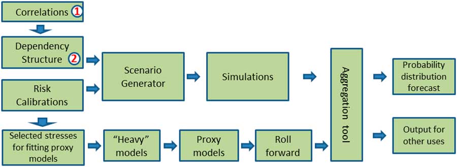
Figure 1 Overview of copula + proxy model approach
1.1.8. The aim of the proxy model is to reflect non-linear responses to changes in risk factors and the interaction between changes in risk factors. The copula-based risk factor simulation model is aimed at producing a full probability distribution forecast by generating a sufficiently large number of scenarios (rather than just a small number of stress tests) which more appropriately reflects the underlying distribution. It permits departure from the assumption of an elliptic distribution by allowing separate choices of the marginal risk factors and the dependency structure between them (i.e. the copula). For example, the copula could be chosen to explicitly include tail dependence and, at least in theory, belong to a non-elliptic family.
1.1.9. The greater complexity of such techniques, the assumptions underlying them and the financial significance of those assumptions means that they are likely to come under greater scrutiny from the users of the models, such as senior management and the Boards of the undertakings. Where the models are to be used to determine regulatory capital requirements under Solvency II, they will also be subject to scrutiny by the supervisory authorities who will expect undertakings to be able to produce evidence that the approach meets all the relevant standards of Solvency II.
1.1.10. Some of the judgements which are likely to come under particular scrutiny include:
-
∙ whether the model which describes the association or dependency between changes in risk factors and its calibration is appropriate – in particular, whether individual parameters (e.g. correlations) can be justified by reference to expert judgement and relevant data (where available) and whether the model and its parameterisation makes adequate allowance for the association between extreme changes in the risk factors (“tail dependence”);
-
∙ whether the fitting error resulting from the use of the proxy model is material and whether appropriate adjustments are made to mitigate the effects of such errors.
1.2 Objective of the Working Party
1.2.1. The objective of the Life Aggregation and Simulations Techniques Working Party was to set out different techniques by which actuaries and insurers could assess and choose between the range of aggregation approaches available. In particular, the Working Party was asked to focus on how insurers could test, communicate and justify those choices to the various stakeholders involved.
1.2.2. The purpose of this paper is to provide UK life insurance actuaries with some examples of techniques which could be used to test and justify recommendations relating to the aggregation approach. Throughout the text we also provide some practical examples of how those techniques may be communicated effectively to stakeholders. (Readers who wish to proceed directly to these sections should refer to section 1.3.) Whilst the techniques involved are more complex than those which have been common under the ICAS framework, the Working Party believes that the underlying concepts can be explained in a manner which is accessible to financially literate stakeholders without going into unnecessary technical detail. We believe that graphical techniques can be a powerful tool in explaining and justifying the assumptions made and include some examples. We have tried to avoid discussion on the technical details and relative merits of specific techniques. However, we have included technical material or appropriate references where we believed this would provide helpful context for the reader.
1.2.3. The Working Party understands that that the “Copula and Proxy Model” method is the most common of the more sophisticated aggregation approaches used in those internal models for whose use some UK life insurers received supervisory approval in December 2015. We have therefore focussed our attention on the challenges faced by actuaries when testing, justifying and communicating choices in relation to this particular approach. We hope the paper will prove useful for actuaries involved in the preparation of internal model applications by undertakings seeking supervisory approval at a future date.
1.2.4. The paper contains examples of some techniques which the Working Party understands have been effective in practice. However, these do not necessarily represent a comprehensive set of tools, use of which will guarantee success. Other techniques may exist which are equally, if not more, effective. Actuaries should choose techniques which are most appropriate to the specific circumstances of the individual undertaking and the users of the model outputs.
1.2.5. The Prudential Regulation Authority (PRA) provided a summary of some aspects of the Quantitative Framework it used when assessing internal model applications during 2015 in two executive updates: “Solvency II: internal model and matching adjustment update” dated 9 March 2015 (PRA, 2015a) and “Reflections on the 2015 Solvency II internal model approval process” dated 15 January 2016 (PRA, 2016). This letter included an overview of the PRA’s quantitative indicators for dependencies. Actuaries involved in the recommendation of a dependency structure and its parameterisation may wish to consult this letter for more information regarding the expectations of the UK supervisory authorities.
1.3 Structure of the Paper
1.3.1. Section 2 provides an overview of the principal stakeholders, their role and interests and ways in which actuaries might approach the communication challenges.
1.3.2. Section 3 describes how the parameters of a copula may be selected using a combination of expert judgement and relevant data (where available). We discuss how the choices may be justified and tested, including the use of statistical and graphical techniques. In particular, we discuss techniques by which allowance can be made for tail dependence. We have focussed on the Gaussian and Student’s t copula as we understand these are the two copulas which have been included in internal models of UK life insurers approved to date. Readers already familiar with the concept of tail dependence may wish to proceed directly to section 3.8. Sections 3.5.1, 3.5.5, 3.6.3, 3.7.1, 3.7.2, 3.8, 3.9 and 3.10 provides some examples of how the underlying concepts and techniques may be communicated, including worked examples based on a specific data set. Section 3.15 discusses “top-down” reasonableness checks.
1.3.3. Section 4 describes the practical aspects associated with fitting and validating a proxy model. We also highlight the key challenges practitioners face in communicating their proxy model results to stakeholders such as senior management, and consider how these can be addressed in sections 4.6.9 and 4.8.
1.3.4. We have assumed that the reader is familiar with the concepts of copulas and proxy models. References to background reading material are provided in the corresponding sections. For the purposes of this paper, we have focussed on the calculation of SCR under Solvency II. The SCR is defined as the Value at Risk (VAR) of basic Own Funds at a confidence level of 99.5% over a 1-year time horizon. The considerations for other measures of economic capital requirements are similar, although the tests and standards of Solvency II may not necessarily apply. Readers should take into account the specific circumstances when applying any of the techniques discussed in this paper.
2 Stakeholders and Communication
In this section we list the principal stakeholders involved in making or reviewing decisions relating to the choice of aggregation techniques and the related assumptions, and the implications for communicating and justifying recommendations to two sets of key stakeholders: members of the Board and the supervisory authorities. Further commentary specific to the dependency structure and proxy models is included in sections 3 and 4, respectively.
2.1 Stakeholders
There are various groups of stakeholders who may be involved in the review of recommendations made regarding aggregations techniques (as well as other components of an Internal Model) and their implementation into the day to day operation of the Internal Model:
2.1.1 Boards
The Board of a company is ultimately responsible for approving the firm’s Internal Model for use. It needs to ensure that on an ongoing basis the design and operations of the Internal Model are fit for purpose; that the model appropriately reflects the company’s risk profile; the model meets the relevant tests and standards and that the output from the model is credible for use in managing the business and for regulatory purposes.
2.1.2 Supervisory authorities
The supervisory authorities will wish to be provided with evidence which demonstrates that the model meets all the relevant tests and standards of Solvency II in order that they are able to approve the model for use in calculating regulatory capital requirements.
2.1.3 Risk committees, senior management
The Board may use the output from reviews by its risk committees to inform its final decision on whether to accept the model or to require changes to it. Senior management will be users of the model in the day to day management of risk in the business and have a role in ensuring it is fit for purpose. Members of senior management will also need to have a detailed understanding of the components of the Internal Model used in their own areas of the business. Senior management may establish technical committees whose membership includes executives from different parts of the business to ensure that recommendations made to the Board on the methodology and assumptions used in the model take appropriate account of business needs in addition to being technically sound.
2.1.4 Risk management function
Under Solvency II, the risk management function is responsible for putting in place an effective risk management system to identify, measure, monitor, manage and report on the risks to which a company is exposed and their interdependencies.
Where an Internal Model has been approved by the supervisory authorities for the calculation of the SCR, the Solvency II Directive states that the risk management function is responsible for the design and implementation of that Internal Model as well as for its testing and validation. This includes the documentation of the Internal Model together with any subsequent changes made to it. The risk management function is also required to analyse the performance of the model and produce corresponding reports. These reports include informing the Board about the performance of the model, areas that need improvement and providing updates on actions aimed at improvement of previously identified weaknesses.
The risk management function is also responsible for the policies relating to the governance of the Internal Model, including the policy for changes to the Internal Model and the framework for validation of the Internal Model.
In practice, the risk management function may delegate some of the day to day activities to the actuarial function, subject to oversight by the risk management function. For example, due to the requirement of Solvency II for independent validation (see section 2.1.6), the design and implementation of the Internal Model together with responsibility for maintaining the related documentation is often delegated to the actuarial function, with oversight provided by the risk management function.
The risk management function is responsible for the developing of proposals for the validation framework for review, challenge and, ultimately, approval by the Board and for the production of regular validation reports to the Board. The resulting validation process will often include a review of the choice of copula and its parameterisation by individuals independent of the development of those proposals. It will also typically include (i) an assessment of the adequacy of the fit of the proxy model by the risk management function or (ii) the definition of a set of tests to be performed by the actuarial function to assess the fit of the proxy model and the criteria for any subsequent adjustments to model outputs with a review of the outcome by the risk management function.
2.1.5 Actuarial function
The actuarial function is often responsible for the design, maintenance, testing and day to day operation of the Internal Model under oversight of the risk management function. The actuarial function will have an interest not only in ensuring the technical soundness of the model and its compliance with the company’s own policies and the relevant regulatory tests and standards, but also that it is appropriate for use in the business. This means that the model should not only be suitable for the calculation of regulatory capital requirements, but also that it does not contain unnecessary areas of prudence which could lead to inappropriate decisions or result in unnecessary constraints on the business. The actuarial function is therefore likely to establish its own “first line” system of review which may include peer review by other technical specialists, technical review forums including other finance experts on areas such as asset liability management, tax or IFRS reporting, and final review by the Chief Actuary. The actuarial function will therefore be highly interested in both the technical soundness of the model as well as ensuring that the outputs it produces provide a realistic measure of the risks.
The actuarial function may also be responsible for maintaining the documentation of the Internal Model, subject to review and approval by the risk management function. This could include preparing papers recommending methodology and assumptions for approval by the Board, together with papers seeking approval from the Board for the results of the Internal Model, including the SCR. These papers should include an assessment of the strengths and limitations of the Internal Model, a description of the significant expert judgements and sensitivities to valid alternative assumptions. In particular, documentation provided to the Board should draw out key judgements relating to the choice of copula, its parameters, how account has been taken of tail dependence, the rationale for those judgements, the associated limitations and sensitivities to valid alternative judgements. The documentation should also draw the attention of the Board to limitations of the proxy model including fitting errors and, where applicable, how these limitations have been allowed for through adjustments to the proxy model result together with the rationale for those adjustments. These judgements should be communicated in a way which is accessible and engaging and which identifies the judgements where the Board can significantly influence the outputs of the model by choosing alternative assumptions.
2.1.6 Independent validation
The Solvency II regulations require regular validation of the Internal Model, including its specification, performance and comparison of its results against actual experience, through a validation process which is independent of those responsible for the development and operation of the model. Responsibility for the validation of the model lies with the risk management function. As indicated in section 2.1.4, the requirement for independence of validation process from those responsible from the development and operation of the Internal Model often means that the latter responsibilities are delegated to the actuarial function under oversight of the risk management function.
Personnel involved in the validation process will be interested in ensuring that the model meets all the relevant tests and standards and is suitable for use in managing the business. Personnel charged with the validation process must regularly report on the outcome of their reviews to the Board. They will therefore wish to have a good understanding of the mathematical basis for the model, detailed evidence which demonstrates that the model it meets the tests and standards of Solvency II, and that the outputs from the model provide a reasonable basis for the measurement and management of risk. They will also be interested in understanding the limitations of the model and circumstances under which it may not be effective, whether an appropriate range of alternative methods have been considered and how the limitations are mitigated.
2.1.7 Internal audit
The internal audit function is responsible for the evaluation of the adequacy and effectiveness of the company’s internal control system, including whether the actuarial function and risk management function have properly performed their respective roles. The internal audit function may therefore carry out its own testing in order to provide assurance to the Board. This could include aspects such as a review of the effectiveness of the processes and controls designed to ensure the Internal Model meets the required tests and standards, the processes around expert judgement (e.g. the selection of correlation assumptions) and whether the process for calibration and adjustment of the output from a proxy model is operated in accordance with the approved specification.
2.1.8 External advisors
Some firms may seek additional assurance from external advisors regarding the design of the model or the underlying assumptions, in particular in specialist areas where the firm feels it does not have sufficient expertise internally or where it wishes to obtain additional insight into market practice.
2.1.9 External auditors
Where the SCR is calculated using an approved Internal Model, according to PRA Consultation Paper CP 43/15 “Solvency II: external audit of the public disclosure requirement” (2015b) (the consultation on which had not been concluded at the time of writing this paper), the PRA does not intend to require the SCR to be subject to external audit. This avoids duplication of the independent validation and the PRA’s own Internal Model approval process. It is for the Boards of such firms to determine the extent of involvement of external auditors in review of the SCR. For example, the Board of some firms may determine that no further external assurance is required. Alternatively, a Board may request external auditors to perform one of a range of possible assurance exercises: (i) review and comment on specific aspects of the SCR calculation; (ii) provide a limited assurance opinion on whether specific items of the SCR have been calculated in accordance with a basis of preparation defined by the firm; or (iii) provide a reasonable assurance opinion on whether the full SCR calculation has been performed in accordance with a basis of preparation defined by the firm. In each case, the basis of preparation would be the specification of the Internal Model approved by the college of supervisors.
2.2 Communication
There is a wide range of potential audiences for communications related to the judgements involved in the aggregation of risks and the Internal Model more widely. Each of these audiences plays a different role and has different interests. In any form of communication, it is important that the communication has a clear purpose, the needs of the audience are taken into account and that essential information is not obscured by material which is not relevant to the decisions being made. The language, style and medium of communication should also be appropriate to the needs of the audience. Some audiences do not require technical details, whilst other audiences may be highly interested in the mathematical theory underlying a particular model. Some audiences may prefer detailed written documentation, whilst for others, the messages may be more effectively conveyed in the form of pictures or diagrams in a slide pack, for example. The structure of any communication is also important. The way any form of communication is organised should be logical and provide a clear path through the material presented in support of the recommendations. Different approaches are therefore needed when communicating with different audiences. It may be appropriate to have several “layers” or “strands” of documentation to meet the needs of different audiences.
The Solvency II regulations provide standards on documentation and the content which must be provided to certain stakeholders. Actuaries should also comply with the relevant professional standards in their communications, in particular with the appropriate Technical Actuarial Standards.
In the remainder of this section, we consider differences in the approach to communication to two key groups of stakeholders: members of the Board and the supervisory authorities.
2.2.1 Board members
Where the Internal Model is used for calculating the SCR under Solvency II, the Board are collectively responsible for ensuring that the Internal Model is fit for purpose and that it meets all the relevant tests and standards. They will therefore wish to make sure that it is appropriate for use in the management of risk in the business as well as for the production of regulatory capital requirements.
This does not mean that members of the Board have to be experts in the mathematics and statistics underlying the capital models. Rather they will need to understand at a high level why a particular model was selected, what that model does, its key features, its strengths and limitations, the significant judgements involved, the related uncertainties and the impacts of reasonable alternative models and assumptions so they can exercise review and challenge where appropriate.
It will therefore be important when explaining recommendations to the Board to focus on the most significant areas of judgement and to avoid technical jargon. Graphical techniques such as scatter plots, charts and histograms provide effective tools to explain and motivate choices in a compact way. Simple worked examples may also be helpful to illustrate concepts. Boards must ensure that they have sufficient understanding of the model, the underlying judgements, their limitations and the sensitivities of the outputs to valid alternative in order to form a view on whether the model is fit for purpose. The Board will also need to be involved in the design of the independent validation process and approve it for use to ensure that proposals have received an appropriate level of technical challenge.
In addition to submitting proposals for approval by the Board at a formal meeting, it will be appropriate to ensure that the Board is well informed in advance of the meeting. A series of educational events, exploring different aspects of the model, may therefore be useful to allow members to build up an understanding and have the opportunity to ask questions prior to making a decision.
Members of Boards are likely to have diverse backgrounds and experience, as well as differing levels of interest in the components of the model. It may therefore be appropriate to offer one-to-one sessions with individual members to provide an opportunity for more detailed exploration of specific areas of interest.
The membership of a Board also changes over time. Firms may therefore wish to maintain an appropriate suite of educational material which can be used to support new directors or as the basis of regular Board “refreshes”.
For the purposes of evidencing effective governance by the Board, it will be appropriate to keep a record of the review and challenge exercised by the Board and track progress against any actions. Firms may also wish to maintain a log of the educational support provided to members of the Board.
2.2.2 Supervisory authorities
Regulators will wish to ensure that the Internal Model meets all the relevant tests and standards of Solvency II prior to approval for use to calculate the SCR. They will therefore expect to be provided with documentation which demonstrates that the model meets the requirements of Articles 120–126 of the Solvency II Framework Directive (2009/138/EC) together with the related requirements of the Delegated Regulations and EIOPA Guidelines. It may therefore be useful to use a checklist or standard documentation template to verify that the documentation to be provided does evidence compliance with all the relevant standards.
The supervisory authorities will want to ensure that the undertaking has a thorough understanding of the techniques used (including the mathematical basis), their limitations and what measures the undertaking has taken to mitigate those limitations. This will include evidence of having taken account of relevant data and the application of appropriate validation tests, including statistical testing, where relevant. The supervisory authorities also have teams of technical specialists whose expertise can be drawn upon to review submissions from firms. Therefore, undertakings may expect to have to present detailed technical documentation to support their methodology.
Regulators will also expect undertakings to have identified all the choices made, the potential impact of alternatives and understand why an undertaking has chosen to go down one particular route rather than another. This includes the identification of the most significant assumptions (e.g. correlations) and a quantification of the impact on the SCR of adopting plausible alternative assumptions.
The selection of a dependency structure and the approach to calibration and adjustment of a proxy model necessarily involve expert judgement. Undertakings should be able to demonstrate that there is a robust and systematic process in place for the selection of those assumptions and their validation, including the adjustment of any assumptions or the outputs to allow for limitations of the model (e.g. the lack of tail dependence in a Gaussian copula; fitting error in a proxy model).
The supervisory authorities will also expect users of the outputs of the model to be aware of any significant limitations of the model so that appropriate account of these limitations can be taken when making decisions informed by the model. They will therefore expect documentation provided to the users to highlight such limitations.
The PRA published some principles on creating good-quality documentation in December 2013 (PRA, 2013). The PRA has also developed a Quantitative Framework which it has used in its assessment of Internal Model applications. It has released some details of the Quantitative Indicators which form part of that framework in two executive director updates dated 9 March 2015 (PRA, 2015a) and 15 January 2016 (PRA, 2016). These updates include an outline of some of the factors considered in the PRA’s assessment of dependency structures. Actuaries involved in the development of internal models may wish to refer to these documents to help understand the PRA’s expectations.
3 Calibration of Copulas and Allowance for Tail Dependence
3.1 Introduction
Most UK life assurance companies that use internal models to calculate their SCR have chosen to use a copula-based approach to aggregation according to recent industry surveys (Ernst and Young LLP, 2015; KPMG LLP, 2015; PricewaterhouseCoopers LLP, 2015; Towers Watson Limited, 2015). Of these, the majority have opted for the Gaussian model with a minority (three, according to the surveys of Towers Watson and KPMG) adopting a Student’s t copula for all or a subset of the risk factors.
The use of the Gaussian or Student’s t copula is likely to be a result of primarily practical considerations:
-
∙ Scarcity of relevant data to reliably inform the choice of a copula family;
-
∙ Transparency – elliptic copulas such as the Gaussian and Student’s t have a correlation matrix as a parameter. A correlation matrix approach to aggregation was commonly used for the Individual Capital Assessment so correlations are likely to be well understood by users of the model;
-
∙ Ease of modelling – these copulas are straightforward to simulate from using spreadsheets or statistical packages and come as standard within some proprietary aggregation tools;
-
∙ Ease of parameterisation – the large number of risk factors, particularly for a more complex group of companies – combined with the previous factors, leads to a preference for models which are no more complex and have as few parameters as is necessary to appropriately reflect the dependencies.
The choice between a Gaussian or Student’s t copula is likely to be determined by a firm’s prior beliefs regarding tail dependence and preference for modelling this explicitly using the Student’s t copula or using the simpler Gaussian copula with appropriate adjustments to the correlation parameters to make allowance for tail dependence.
In this section we assume that the choice to use either a Gaussian or a Student’s t copula has already been made (i.e. the choice of dependency structure in the box labelled ‘2’ in Figure 1). We focus on techniques that may be used to inform and justify the selection of the parameters of these two copulas (i.e. the correlations and any other parameters in the box labelled ‘1’ in Figure 1). In particular, we consider how allowance can be made in the parameterisation, explicitly or implicitly depending on the choice of model, for tail dependence.
We have assumed that the reader is familiar with the basics of copulas. There are numerous good references. McNeil et al. (Reference McNeil, Frey and Embrechts2015), Cherubini et al. (Reference Cherubini, Luciano and Vecchiato2004), Joubert & Dorey (Reference Joubert and Dorey2005), Sweeting & Fotiou (Reference Sweeting and Fotiou2013) and Shaw et al. (Reference Shaw, Smith and Spivak2011) provide accessible accounts in a finance context. Nelsen (Reference Nelsen1998) and Joe (Reference Joe2015) are standard, but more technical, reference works. The paper by Demarta & McNeil (Reference Demarta and McNeil2005) provides a comprehensive review of the Student’s t copula while the paper by Aas (Reference Aas2004) provides a practical introduction to simulation from copulas.
3.2 Overview of Section
In this section, we cover the following:
-
1. Bottom-up parameterisation:
-
a. Use of data to inform the parameterisation
-
i. Inspection of the data using graphical techniques – section 3.5.1.
-
ii. Different time periods – section 3.6.1.
-
iii. Confidence intervals – section 3.6.2.
-
-
b. Parametric fitting techniques
-
i. Method of moments (MoMs) type approaches based on first-order rank statistics – section 3.5.3.
-
ii. Maximum pseudo-likelihood (MPL) – section 3.5.4.
-
-
c. Allowing for tail dependence
-
i. Definition and communication – section 3.7.
-
ii. Coefficients of finite tail dependence – section 3.8.
-
iii. Targeting conditional probabilities – section 3.9.
-
iv. Techniques based on matching high-order rank statistics – section 3.10.
-
-
d. Overlay of expert judgement and selection of assumptions in the absence of relevant data – sections 3.12 and 3.13.
-
-
2. Adjustments for internal consistency (positive semi-definiteness (PSD)) – section 3.14.
-
3. Top-down validation – section 3.15.
We end the section by commenting briefly on techniques for testing the choice of copula.
Readers who are already familiar with the estimation of correlations and tail dependence may wish to proceed directly to section 3.8.
3.3 Relevance of Data and Statistical Techniques
Given the scarcity of data, even for pairs of market risks, one may suspect it would be a futile exercise to apply statistical techniques to whatever data are available in order to inform the choice of assumptions. Whilst the uncertainty in parameters derived using data means that the selection of copula parameters should never be a purely data-driven exercise and therefore necessarily relies on expert judgement, use of statistical techniques can help inform the choice of assumptions and support the judgements made.
The statistical quality standards of Solvency II also indicate that relevant data should be used where possible. For example, Article 231 of the Solvency II Delegated Regulations (2015) states “… no such relevant data [is] excluded from the use in the internal model without justification”. Article 234 of the Delegated Regulations requires that “the assumptions underlying the system used for measuring diversification effects are justified on an empirical basis”. Article 230(2)(c) of the Delegated Regulations states “assumptions shall only be considered realistic … where they meet all of the following conditions … insurance and reinsurance undertakings establish and maintain a written explanation of the methodology used to set those assumptions”. (See Appendix B for the full text of Article 230.)
The Working Party has interpreted these regulations as requiring an undertaking to have a documented process for the selection of the copula parameters that includes an appropriate analysis of the relevant data combined with the use of expert judgement.
3.4 Communication and Validation
When explaining statistical concepts to stakeholders as well as the selection and validation of assumptions informed by these techniques, members of the Working Party has found that visualisation techniques tend to result in the greatest level of engagement. They can be used in explaining technical terms in a way which is more readily accessible than formulae. They also provide a compact format for illustrating the choices which is straightforward to interpret. Moreover, the effect of a different set of assumptions can be illustrated by superimposition on the same chart or even using simple animation techniques (e.g. by flicking through a set of slides showing graphically how the output of the model compares to data as the parameters of the model are varied). However, one of the drawbacks of visualisation techniques is that they naturally tend to be useful only in two or three dimensions. Nevertheless, this limitation is often accepted and combined with expert judgement to choose correlation assumptions.
Where the analysis is less amenable to visualisation (e.g. parametric fitting techniques such as those described in section 3.5.5), the level of information required may vary more according to the stakeholder. Personnel responsible for independent validation and the supervisory authorities will expect documentation to evidence a detailed understanding of the technique, its strengths and its limitations, and provide sufficient evidence to demonstrate the model and assumptions meet the statistical quality standards of Solvency II. The Board is ultimately responsible for the appropriateness of the design and operations of the Internal Model. Therefore, whilst the Board and senior management do not need to be experts on the underlying mathematics, they will want to understand at a high level how a copula works; the significant choices and judgements involved in selecting and parameterising a copula (such as making allowance for tail dependence) and their implications; the impact of alternative but nonetheless reasonable assumptions and the process by which those have been validated. An explanation of a copula in terms of matching ranks of values of the marginal distributions according to an algorithm which reflects the dependency structure and illustrating this concept by means of scatter plots of the copula may be helpful (see e.g. Simulation and Aggregation Techniques Working Party, 2015). The Board and senior management may also wish to see the rationale for certain key assumptions explained at a high level, included the general reasoning and economic arguments supporting correlations (see section 3.12) and the types of real-life scenarios that can give rise to losses of similar magnitude to the SCR (see section 3.15).
In order to illustrate how the visualisation and quantitative techniques described in this section may be used in the communication and justification of assumptions, we have provided a number of worked examples of approaches which we understand have been effective in discussions with some stakeholders. The majority of these examples are based on a set of three risk factors representing monthly increases in equity values (EQ), corporate bond spreads (CR) and the first principal component of the UK nominal government bond yield curve (PC1). This data set has been chosen as it represents a set of risk factors to which most life assurance undertakings have some exposure and for which the data available are comparatively rich. A description of the data is provided in Appendix A.1.
Irrespective of the data, it is important that the choice of assumptions can be explained and justified by economic arguments or general reasoning. Such arguments form an important part of the validation of any assumption suggested by data and may be more accessible to some stakeholders.
It is common to build up the parameterisation of a copula using a “bottom-up” approach which considers relationships between pairs of risk factors. It is therefore important that the final set of assumptions is coherent and “stacks up” collectively. We discuss top-down validation in section 3.12 but note here that one of the most significant advantages of a simulation-based approach to capital aggregation is the ability to identify one or more “real life” individual scenarios giving rise to losses of magnitude similar to the SCR. These scenarios (expressed as changes in risk factors in terms which are accessible, e.g. increases in life expectancy at specific ages, reductions in interest rate at specific terms) can allow stakeholders to form a view of whether the model outcomes are consistent with the risk profile of the business and so assist in the validation of assumptions.
Finally, we observe that in the selection of copula parameters, the boundary between “calibration” and “validation” is somewhat blurred. This is because “calibration” necessarily involves the exercise of judgement, so the process of calibration itself involves thinking through the rationale and possible alternatives. For example, one could “calibrate” a correlation using a single statistical process, such as the relationship described in equation (1), use the approach described in section 3.8 to “validate” and, if appropriate, adjust the original calibration, with an overall sense check using the approach of section 3.15. Alternatively, the approach described in section 3.8 could just as well be described as one part of the calibration process.
3.5 Bottom-Up Approach to Parameter Selection
3.5.1 Data inspection
A first step in illustrating dependency is through plots of time series and scatter plots. These relatively simple charts are often the simplest and most effective tool in demonstrating evidence of association to stakeholders and motivating subsequent choices.
Scatter plots of the data can assist in:
-
∙ The identification of the presence of a relationship.
-
∙ The nature of that relationship (e.g. the sign and broad magnitude of any correlation, the extent of any symmetry or lack of it, and any clustering of extreme values that may indicate the presence of tail dependence).
-
∙ Identification of any data points, which could be outliers.
Charts of both the raw observations and pseudo-observations are useful. The pseudo-observations (defined in Appendix A.2) use a non-parametric transformation of ranks to filter out the marginal distributions and can be compared with scatter charts of standard copulas.
As noted in Shaw et al. (Reference Shaw, Smith and Spivak2011), by excluding the time dimension, scatter plots mask temporal effects which may be present in the data and which one may wish to take in account when selecting assumptions (e.g. trends or a change in regime).
Figure 2 shows a time series plot of equity returns versus increases in credit spreads. Figure 3 shows scatter plots of pairs of increases in value of our three risk factors and the corresponding pseudo-observations.

Figure 2 Monthly equity returns and increases in credit spreads over period 31 December 1996 to 31 December 2014

Figure 3 Equity returns and credit spreads raw and pseudo-observations
Figure 2 shows no obvious trend in the relationship between equity returns and credit spreads. There is an obvious anti-symmetry in the “peaks” with increases in credit spreads frequently being mirrored by negative equity returns. The strong negative correlation is also apparent in Figure 3. The chart of pseudo-observations for EQ/CR shows some clustering in the upper left and lower right tails along the “−45% ray” – that is, extreme falls in equity values show a greater tendency to be accompanied by extreme increases in credit spreads (and vice versa). However, it also shows some clustering along the other diagonal (the “+45% ray”) giving rise to “star” shape. This behaviour is typical of a Student’s t copula with a low degrees of freedom parameter and indicates the presence of “arachnitude” – see section 3.10.
From the charts of pseudo-observations, at least visually, the assumption of an elliptic copula for each pair does not appear unreasonable.
3.5.2 Parametric fitting techniques
There are various statistical techniques for estimation of the copula parameters which extend the MoM or maximum likelihood estimate (MLE) method that are familiar in fitting models for one-dimensional random variables. We describe these techniques briefly here. Readers are referred to standard texts, for example, section 7.5 of McNeil et al. (Reference McNeil, Frey and Embrechts2015), for further details.
3.5.3 MoMs type approaches
These are based on (first order) rank invariants of the copula such as Spearman’s rank correlation or Kendall’s τ statistic.
For the d-dimensional Gaussian copula, one can calculate Spearman’s rank correlation or Kendall’s τ for the sample data and invert to solve for the correlation parameter using the formulae below:
 $$\rho \,\, {\equals}\, \,2\sin \left( {{{\pi \rho _{S} } \over 6}} \right)$$
 $$\rho \,\, {\equals}\, \,\sin \left( {{{\pi \rho _{\tau } } \over 2}} \right)$$
where, for a given pair of risk factors, ρ S is the Spearman’s rank correlation, ρ τ the Kendall’s τ statistic and ρ the corresponding parameter of the correlation matrix underlying the copula. The relationship in equation (1) is precise only for the Gaussian copula, although in practical situations, it does not appear to lead to significantly different conclusions.
The approach based on the relationship involving Kendall’s τ statistic described by equation (2) (the “inverse Kendall’s τ” technique) holds more generally for any elliptic copula such as the Student’s t copula. However, pairwise inversion of the Kendall’s τ statistic using equation (2) may not produce a PSD copula correlation matrix. It may therefore be necessary to adjust the resulting matrix using techniques such as those described in section 3.14 to obtain a PSD correlation matrix. This technique also results only in values for the correlation matrix. Other techniques such as maximum likelihood estimation or use of higher order rank statistics such as those described in section 3.10 must be used to estimate the degrees of freedom parameter.
3.5.4 Maximum likelihood approaches
There are two slightly different approaches to the estimation of copula parameters using maximum likelihood techniques:
-
(a) Inference from margins (IFM) approach – see Joe (Reference Joe2015)
This approach assumes parametric models for each of the distributions of changes in individual risk factors as well as for the copula. The usual maximum likelihood approach, given a set of sample data for changes in the risk factors, would then be to express the likelihood (or log likelihood) of the joint distribution as a function in the parameters of the copula and all the marginal distributions. This will generally result in a high-dimensional space in which to seek a solution.
The IFM approach splits this optimisation process into two separate steps:
-
∙ First, the parameters of each of the one-dimensional marginal distributions of changes in risk factors are estimated using maximum likelihood.
-
∙ The fitted parameters of the marginal distributions are then kept fixed so that the (log) likelihood function is then expressed in terms of the copula parameters only. The values of these parameters are then chosen to maximise the (log) likelihood.
The values of the copula parameters therefore depend on the models and parameters chosen for the individual risk factor distributions.
-
-
(b) MPL – see Genest & Rivest (Reference Genest, Rémillard and Beaudoin1993) and McNeil et al. (Reference McNeil, Frey and Embrechts2015)
This method avoids making assumptions about the marginal distributions by using non-parametric techniques to estimate their distributions. The sample data are replaced by the corresponding “pseudo-observations” – see Appendix A.2 for definitions. The corresponding pseudo-observations are then used as inputs to the probability density function of the copula when forming the (log) likelihood function. The resulting likelihood function then depends only on the parameters of the copula and, unlike the IFM approach, not on the assumed models and parameters of the marginal distributions. The copula parameters can then be selected using optimisation techniques.
3.5.5 Worked example
We have fitted correlation parameters (“ρ”) and degrees of freedom parameters (“Nu”) of the Gaussian and Student’s t copulas to our data set using:
-
(a) the inverse Kendall’s τ technique to estimate ρ (with MLE to estimate Nu) using the “QRM” package in R;
-
(b) the MPL method using the “copula” package of R.
In both cases, we have fitted to pairs of risk factors as well as the triple. Tables 1 to 4 show the results.
Table 1 Bivariate

Table 2 Trivariate

Table 3 Bivariate – Maximum Pseudo-Likelihood
Table 4 Trivariate – Maximum Pseudo-Likelihood
Inverse Kendall’s τ
MPL
We note the following:
-
∙ Fitting a Gaussian copula using either technique results in a correlation parameter which is appropriate to the full distribution. The resulting value of the correlation is identical to that fitted to a Student’s t model if the inverse Kendall’s τ method is used. It does not differ significantly from the corresponding parameter for a Student’s τ copula if the MPL approach is used, even where the degrees of freedom parameter is low. This suggests that, if using a Gaussian copula, further adjustments to the correlations parameter may be required to allow for the effect of tail dependence in the extreme tail – see sections 3.8 and 3.9.
-
∙ For example, for EQ/CR, both the MPL and MoM fit for the bivariate t copula produce a degrees of freedom parameter of <3. However, the correlation parameter of the bivariate Gaussian and bivariate Student’s t fitted using the MPL technique only differ by <3 percentage points (−48.8% compared to −46.5%, respectively).
-
∙ Where a Student’s t copula is fitted for each pair of risk factors separately, the degrees of freedom parameters for the different pairs vary significantly. The degrees of freedom parameter in the trivariate case (4.51) is in some sense an “average” of the three bivariate values (2.60, 9.40 and 6.08).
3.6 Estimation of Correlation Parameters in Practice
In practice, the choice of correlation parameters is not a mechanistic, data-driven process. Even where data are available (principally for market risks), one has to make a choice of the data set to use: the data series itself, the time period used and frequency at which the data are selected. Consideration must also be given to consistency with the data used for the calibration of marginal risk distributions.
In order to analyse correlations, the data for the two risk factors has to be coincident – that is, the time period and sampling frequency used must be identical. Even for pairs of market risks, the periods for which coincident data are available is relatively short. For example, the financial times stock exchange All Share Index began in 1962 and one of the most commonly used indices of credit spreads began at the end of 1996. These relatively short periods of coincident data will contain limited information about extreme events.
Different choices of data sets will generally lead to different values. For example, an analysis of the correlation between two risk factors will produce differing values over different time periods – see section 3.6.1. Any estimates produced from a finite data set will also be subject to parameter mis-estimation error.
Thus, whilst an analysis of the data which is available can assist in informing the choice of a correlation parameter, in practice it is essential to overlay this analysis with expert judgement – see section 3.12. Where there is no or extremely scanty data available, which is the case for most correlations involving non-market risks, it is essential to make use of expert judgement and general reasoning in selecting the assumption – see section 3.13.
3.6.1 Different time periods
In practice, the correlation between increases in two risk factors varies over time. Judgement is therefore required in selecting both the period of time on which the estimate is based and any allowance made for any uncertainty in the estimate. Note that the latter is a margin for prudence in the estimate of the copula parameter. In the case of a Gaussian copula, this differs conceptually from any further allowance which may be made to adjust for the absence of tail dependence, although the outcome may be similar. We discuss adjustments to the parameters of a Gaussian copula for tail dependence in sections 3.8 and 3.9.
Charts of correlations over different time periods may be helpful in illustrating the resulting uncertainty to stakeholders in a manner which is compact and amenable to explanation, for example, by pointing out the consequences of certain extreme market events. Such charts may also help identify any potential trends in correlations which the undertaking may wish to take into account when selecting assumptions.
For example, one might produce a chart showing rank correlations over different windows of time, such as:
-
(a) From a varying start date to a fixed end date (e.g. the end of the period for which data are available).
-
(b) From a fixed start date (e.g. the start of the period for which data are available) to a varying end date.
-
(c) Over a window of fixed length moving through the data period.
-
(d) Some other set of time periods chosen to test differences in behaviour.
Under (c), the length of the window could be selected using judgement as being sufficient to form a view on “short-term” correlations and give an idea of how correlations could vary between benign and stressed conditions. The choice of window is a compromise between the length of the window and the uncertainty in the resulting estimates. A longer window will result in a lower sample error but on the other hand may not pick up short-term behaviour. Modellers who use this approach may wish to assess the effect of using different window lengths, particularly where it is used to inform material assumptions.
The charts produced may also be enriched by superimposing information about confidence intervals which may be derived using techniques such as those described in section 3.6.2.
3.6.2 Confidence intervals
It may be useful to illustrate the uncertainty in-sample estimates using confidence intervals. There are a number of techniques available, for example:
-
(i) Fisher Z-transform. This uses asymptotic properties of the distribution of transformed data to provide analytic formulae for the upper and lower bounds of a confidence interval. There are various versions of the formulae, which are intended to adjust the result to allow for the finite sample size.
-
(ii) Bootstrapping. A large number of synthetic data sets is generated by re-sampling the original data with replacement. The rank correlation for each of the synthetic data sets is then calculated. This process generates a large number of simulated values of the rank correlation from which appropriate percentiles may be drawn to determine the confidence interval.
The paper by Ruscio (Reference Ruscio2008) provides a useful survey of these approaches. Functions provided in some statistical packages such as R also produce confidence intervals.
3.6.3 Graphical tools
Figure 4 is an example of a chart of type (a) described in section 3.6.1 for the Spearman’s rank correlation of our EQ/CR data set from a varying start date to a fixed end date of 31 December 2014. We have superimposed 95% confidence intervals produced using both the Fisher Z-transform (described by formula (3) of Ruscio, Reference Ruscio2008) and bootstrapping techniques (with 1,000 simulations). Visually, in this case, the confidence intervals produced by the different techniques are almost indistinguishable.

Figure 4 Equity returns and credit spreads Spearman’s rank correlation – chart of type (a); CI=confidence interval
Note that this approach provides information only about the rank correlation – a scalar statistic which is “global” – rather than relevant to a specific area of the joint distribution such as the tail. It is therefore more useful in informing one’s best estimate view of a correlation. If it is considered appropriate to include a margin for uncertainty in the correlation, one potential approach would be to use the confidence intervals as a guide to select a higher or lower value for the correlation, taking into account the exposures in the “biting scenario”. (The “biting scenario” is a scenario which, in some sense, represents the average simulated scenario which gives rise to losses equal in magnitude to the SCR. For example, some undertakings produce such a scenario by applying a smoothing process to simulated scenarios, the ranks of whose corresponding losses lie in a “window” around the SCR.)
Inspection of rolling short-term correlations such as using charts of type (c) may be useful to inform views of correlations in “stressed circumstances” and of any further allowance for tail dependence which may be appropriate. However, we note that the copula used in the calculation of the SCR (and the tail dependence embedded within it) is a static quantity. The change in correlation over time is conceptually different to tail dependence.
Figure 5 illustrates correlations for a rolling 24 month window for our EQ/CR data set. It shows the correlation reaching almost −75% for periods beginning in 2009 during the financial crisis.
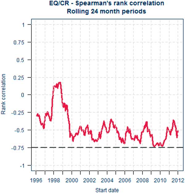
Figure 5 Equity returns and credit spreads – correlations for rolling 24 month periods, start dates 31 December 1996 to 31 December 2012
One crude method of allowing for tail dependence would be to select an assumption based on confidence intervals or “stressed correlations” informed by charts such as Figures 4 or 5. However, as noted, these are conceptually different from tail dependence so such an approach would have to be carefully justified. Alternative approaches are discussed in sections 3.8, 3.9 and 3.10.
3.6.4 Rounding
To reflect the uncertainty in the chosen parameter values and the use of judgement, as well as for the practical reason of avoiding the frequent re-calibration of a large set of parameters, it is a common practice to round correlation assumptions according to a convention chosen by the undertaking (e.g. round to integer multiples of 10%). This rounding may lead to internal inconsistencies in the “raw” correlation matrix with adjustments required to make it PSD prior to use in simulation – see section 3.14.
The rounding convention is itself a choice which should be justified. A notch size which is too small may be spuriously accurate. On the other hand, a notch size which is too large may provide insufficient granularity and could lead to unnecessary prudence or unintended imprudence as well as inconsistencies in the raw matrix which require larger adjustments to produce a PSD matrix.
3.7 Tail Dependence
In this section, we recall the definition of the coefficients of tail dependence and its significance in terms of joint and conditional probabilities of the simultaneous occurrence of extreme events in two or more risk factors. The latter provide a route to explaining the meaning of tail dependence to stakeholders – see section 3.7.2. The approach we adopt is based on the coefficient of finite tail dependence. As we will see in section 3.8 this function can help to inform the choice of correlation parameters for a Gaussian copula. Readers who are already familiar with these concepts may wish to move directly on to section 3.8.
Definition – coefficients of finite tail dependence
The coefficients of upper or lower finite tail dependence are functions λ U and λ L defined for q∈[0, 1] as follows:
 $$\lambda _{U} (q)\,\, {\equals}\, \,{\rm Pr}\left( {F_{X} \left( X \right)\,\gt\,q\left| {F_{Y} } \right.\left( Y \right)\,\gt\,q} \right)\,\, {\equals}\, \,{{{\rm Pr}\left[ {F_{X} \left( X \right)\,\gt\,q {\rm \ AND\ } F_{Y} \left( Y \right)\,\gt\,q} \right]} \over {Pr\left[ {F_{Y} \left( Y \right)\,\gt\,q} \right]}}$$
 $$\lambda _{L} (q)\,\, {\equals}\, \,{\rm Pr}\left( {\left( {F_{X} \left( X \right)\,\lt\,(1{\minus}q)\left| {F_{Y} } \right.\left( Y \right)\,\lt\,(1{\minus}q)} \right)} \right.\,\, {\equals}\, \,{{{\rm Pr}\left[ {F_{X} \left( X \right)\,\lt\,\left( {1{\minus}q} \right) {\rm \ AND\ } F_{Y} \left( Y \right)\,\lt\,\left( {1{\minus}q} \right)} \right]} \over {{\rm Pr}\left[ {F_{Y} \left( Y \right)\,\lt\,\left( {1{\minus}q} \right)} \right]}}$$
That is the coefficient of finite upper tail dependence function λ U (q) is the probability that a value of X exceeds the q th percentile of X given that a value of Y has been observed which exceeds the q th percentile of Y. λ U (q) is a measure of the probability that X takes an extreme high value given that Y takes an extreme high value.
Similarly, λ L (q) is the probability that a value of X is less than the (1−q)th percentile of X given that a value of Y has been observed that is less than the (1−q)th percentile of Y. λ L (q) is a measure of the probability that X takes an extreme low value given that Y takes an extreme low value.
Note that both λ U (q) and λ L (q) are probabilities (not correlations) and so take values in the interval [0, 1].
Definition – coefficients of tail dependence
The coefficients of upper and lower tail dependence λ U and λ L are limiting values of coefficients of finite tail dependence given by:
 $$\lambda _{U} \,\, {\equals}\, \, \mathop{{\lim }}\limits_{{q\to1{\minus}}} \lambda _{U} \left( q \right)$$
 $$\lambda _{L} \, {\equals}\, \mathop{{{\rm lim}}}\limits_{{q\to1{\minus}}} \lambda _{L} \left( q \right)$$
We have used a slightly different definition of the coefficients of lower finite tail dependence than the conventional one to ensure that, for a radially symmetric copula (such as the Gaussian or Student’s t), values of lower and upper finite tail dependence are equal for a given value of q. This presentation will prove convenient in section 3.8 in the application of graphical methods.
3.7.1 Communicating the concept of tail dependence
Figure 6 shows a graphical method for illustrating the meaning of the coefficient of lower tail dependence.
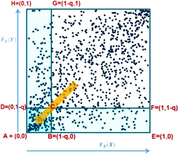
Figure 6 Coefficient of lower (finite) tail dependence
In the diagram, the events have been expressed on a quantile (or rank) scale. The coefficient of lower finite tail dependence evaluated at q, λ L (q), is the ratio of:
-
(i) The proportion (or probability) of events in the square ABCD; to
-
(ii) The proportion (or probability) of events in the rectangle AEFD
The probability of events occurring in the rectangle AEFD is (1−q), by definition.
As the events become more extreme (i.e. q increases), the square ABCD and the rectangle AEFD shrink. The coefficient of tail dependence is the limiting value of the ratio of the proportion of events that occur in the shrinking square to the proportion of events that occur in the shrinking rectangle.
Note that the probability of events occurring in the vertical rectangle ABGH is also by definition (1−q). The definition of λ L (q) in equation (4) is therefore clearly symmetric in X and Y.
The coefficient of finite upper tail dependence, λ U (q), may be illustrated in an analogous way.
It is a standard result that the coefficients of tail dependence of a Gaussian copula are zero while those of a Student’s t copula are non-zero. For example, the coefficient of tail dependence of a bivariate Student’s t copula with correlation parameter ρ and ν degrees of freedom is given by:
 $$2t_{{\nu {\plus}1}} \left[ {{\minus}\sqrt {\left( {\nu {\plus}1} \right)\left( {1{\minus}\rho } \right)\,/\,\left( {1{\plus}\rho } \right)} } \right]$$
where t ν+1 is the cumulative distribution function of a standard Student’s t distribution with (ν+1) degrees of freedom – see equation (7.38) of McNeil et al. (Reference McNeil, Frey and Embrechts2015).
3.7.2 Communicating the implications of tail dependence
So what does the presence of tail dependence mean in practice? The definition of the coefficient of tail dependence in terms of a limiting value makes the concept more difficult to explain to stakeholders. When explaining the implications of tail dependence to stakeholders, it may therefore be more useful to provide some simple quantitative indicators of what different copula models and parameters mean for the likelihood of “extreme events happening at the same time”, by illustrating the consequences in terms of joint exceedance probabilities or conditional probabilities. As we shall see in section 3.8 the use of conditional probabilities in the form of the coefficient of finite tail dependence provides a useful graphical tool to inform the selection or validation of parameters.
3.7.2.1 Joint exceedance probabilities
Tables 5 to 7 are based on tables 7.2 and 7.3 of McNeil et al. (Reference McNeil, Frey and Embrechts2015), although we have chosen parameters more typical of those commonly seen in a life insurance context. They show:
-
∙ A comparison of joint exceedance probabilities at differing percentiles produced by a bivariate Student’s t copula with those produced by a bivariate Gaussian copula for various correlation and degrees of freedom parameters.
-
∙ Each table shows the probabilities for the Gaussian copula and the factors by which those probabilities must be multiplied to obtain the corresponding probabilities for the Student’s t copula. For example, assuming a correlation parameter of 50%, the probability that both risk factors exceed their “1 in 100 year” values at the same time under a Student’s t copula model with 5 degrees of freedom is twice that under a Gaussian copula model. An event with a probability of 0.00129 or around 1 in 770 years under the Gaussian copula now has a probability of 1 in 385 years under the Student’s t copula. See the highlighted cells in the table.
-
∙ Looking at Table 5 for a correlation of 0%, the probability of both variables simultaneously exceeding their 95th percentiles is 0.25% under a Gaussian model. However, under a Student’s t copula with 5 degrees of freedom, the probability increases by a factor of 2.24 to 0.56%. An event with probability <1 in 200 under the Gaussian model (1 in 400) has a probability >1 in 200 under the Student’s t model (around 1 in 180).
-
∙ Tables 6 and 7 provide a comparison of joint exceedance probabilities for d-tuples of risk factors to illustrate how tail dependence influences behaviour in higher dimensions. The tables show the joint exceedance probabilities for the Gaussian copula and corresponding multiples for the Student’s t copula with various degrees of freedom. For each copula, the off-diagonal correlation parameters are all equal to the value shown. We show values for 2, 5, 10 and 25 dimensions and at the 75th and 90th percentiles (to illustrate dependence on event severity).
Table 5 Joint Exceedance Probabilities (Gaussian and Bivariate Student’s t Copula Shown as Multiples of the Gaussian)
DOF=degrees of freedom.
Table 6 Joint Exceedance Probabilities at 75th Percentile

DOF=degrees of freedom.
Table 7 Joint Exceedance Probabilities at 90th Percentile

DOF=degrees of freedom.
For example, taking 90th percentile (or “1 in 10 year” events) in each risk factor and assuming a correlation parameter of 25%, a simultaneous event in ten risk factors, each of which is at least as severe as a 1 in 10 year event, is 5.7 times more likely if they follow a Student’s t model with 5 degrees of freedom compared to a Gaussian. The equivalent multiplier for two dimensions is 1.27. See the highlighted cells in the table using 25% correlation.
The results illustrate the importance of considering tail dependence and making appropriate adjustments to the copula parameters to allow for this. As we saw in section 3.5.5, the application of standard fitting techniques can produce very similar correlation parameters for a Gaussian and Student’s t model. Yet, as shown by Tables 5 to 7, the two models can produce very different joint exceedance probabilities at extreme percentiles. When calculating the SCR or using an Internal Model to generate other outputs at extreme percentiles, it is therefore essential to consider tail dependence when selecting the parameters of the model. The selection of copula parameters necessarily involves expert judgement. We discuss some techniques for informing that judgement in the case of the Gaussian and Student’s t copula in sections 3.8, 3.9 and 3.10.
3.7.2.2 Conditional probabilities
An alternative approach to illustrating the effects of tail dependence is to show the effects on conditional probabilities (i.e. the coefficients of finite tail dependence). For example, Table 8 shows the coefficients of finite tail dependence for a bivariate Gaussian copula and bivariate Student’s t copulas with 5 and 10 degrees of freedom linking random variables X and Y with a common value of 50% for the correlation parameter. It shows that the probability of Y exceeding its 97.5th percentile value given that X has exceeded its 97.5th percentile value under the assumption of Student’s t copula with 5 degrees of freedom is 156% of that assuming a Gaussian model.
Table 8 Coefficients of Finite Tail Dependence (Bivariate Gaussian and Bivariate Student’s t Copulas, 5 and 10 Degrees of Freedom)

DOF=degrees of freedom.
Note that the ratios of the conditional probabilities of the Student’s t model to the Gaussian model in Table 8 are equal to the corresponding ratios of joint exceedance probabilities in Table 5. This is because in the conditional probabilities in numerator and denominator are both obtained by dividing the joint exceedance probability by the probability of Y exceeding the corresponding percentile – see equation (3).
From examining the ratios of joint exceedance probabilities in the tables, it is apparent that, for an equi-correlation matrix and all other things equal, the amplifying effect of tail dependence increases as:
-
∙ The percentile of the joint event increases (where the joint event is assumed to be a combination of equi-probable events in each of the risk factors).
-
∙ The correlation parameter reduces.
-
∙ The degrees of freedom parameter reduces.
-
∙ The number of dimensions increases.
3.7.2.3 Charts of coefficients of finite tail dependence
The implications of tail dependence for conditional probabilities can be summarised compactly using simple charts showing the value of the coefficients of upper and lower tail dependence λ U and λ L as a function of the percentile q. We will see in section 3.8 that, where a Gaussian model has been chosen, such charts can provide a useful tool in explaining to stakeholders the selection of correlation assumptions and adjustments made to those parameters to allow for tail dependence.
Figure 7 illustrates the behaviour of the coefficient of finite tail dependence for the bivariate Gaussian copula and bivariate Student’s t copulas with 5 and 10 degrees of freedom with correlation parameters of 25%, 50% and 75%. (The right hand plot in Figure 7 is restricted to events more extreme than the 90th percentile.) As these copulas are radially symmetric, the charts of λ U and λ L are coincident.
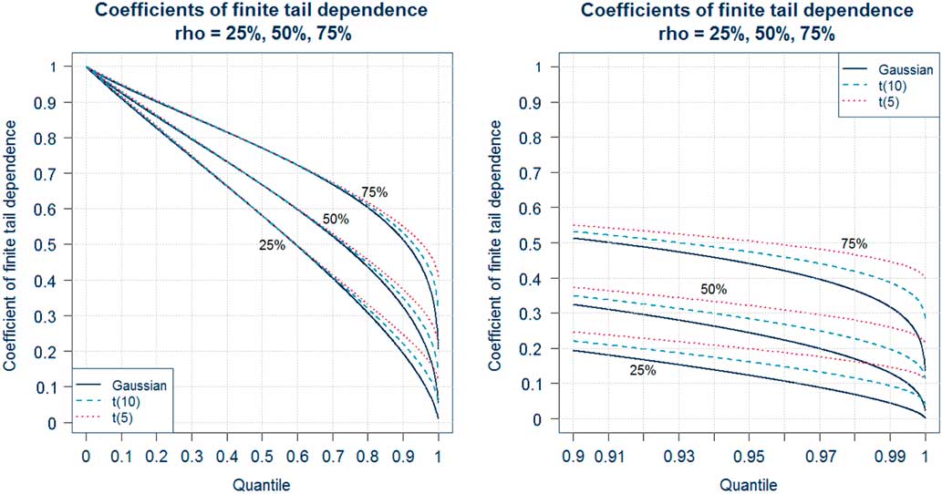
Figure 7 Coefficients of finite tail dependence, ρ is correlation (expanded view 90th percentile on the right)
The following is apparent from the charts:
-
∙ The correlation parameter is the principal factor that determines conditional probabilities.
-
∙ There is little difference in conditional probabilities in the body of the distribution.
-
∙ However, differences in the shape of the functions become apparent in tails. For a given correlation, the coefficient of finite tail dependence is greater for a Student’s t copula than for the Gaussian copula and increases as the degrees of freedom parameter reduces.
-
∙ The coefficients of finite tail dependence tend to zero for the Gaussian copula but to non-zero values for the Student’s t copula.
A coefficient of tail dependence of zero does not imply that extreme changes in one risk are less likely to be accompanied by extreme changes in another. In the case of the Gaussian copula, a positive correlation assumption between increases in X and increases in Y means that, on average, large increases in Y will tend to occur if a large increase in X has occurred. Recall that the conditional distribution is given by:
 $$\left. Y \right|X\,\sim\,N\left( {\mu _{Y} {\plus}\rho {{\sigma _{Y} } \over {\sigma _{X} }}\left( {X{\minus}\mu _{X} } \right),\left( {1{\minus}\rho ^{2} } \right) \sigma _{Y}^{2} } \right)$$
A large value of X results in a large value of the mean of Y|X and therefore an increased tendency for Y to take large values.
A coefficient of tail dependence equal to zero also does not necessarily mean that the corresponding pair of risk factors are asymptotically “independent in the tail”, even for a Gaussian copula. See for example, section 2.2 of Malevergne & Sornette (Reference Malevergne and Sornette2003).
3.8 Selection of Correlation Assumptions Using Coefficients of Finite Tail Dependence
3.8.1 Introduction
In this section, we present one possible technique that could be used to adjust correlation parameters of a Gaussian copula to allow for tail dependence. The technique is based on work by Venter (Reference Venter2002, Reference Venter2003a, Reference Venter2003b) and involves comparing the empirical coefficients of finite tail dependence derived from sample data (explained in section 3.8.2) with the coefficients of finite tail dependence produced by the proposed model and its parameters.
The technique uses the charts introduced in section 3.7.2.3 which permits various assumptions to be tested against the data and the outcome presented graphically. This approach may be more accessible to some stakeholders, leading to greater engagement in the process of selecting or validating parameters.
3.8.2 Empirical coefficients of finite tail dependence
The empirical coefficient of lower finite tail dependence functions is obtained by taking the ratio of the number of pseudo-observations in our sample that fall into the shaded square ABCD to the number of pseudo-observations that fall into the rectangle AEFD in Figure 6. For example, if we have a sample of N observations (X
i
, Y
i
)i=1, … , N from (X,Y) with ranks (R
i
,S
i
) then the empirical lower tail dependence function $\hat{\lambda }_{L} \left( q \right)$
is given by the ratio:
$\hat{\lambda }_{L} \left( q \right)$
is given by the ratio:
 $$\hat{\lambda }_{L} \left( q \right)\, {\equals}\, {{\,\#\,\left\{ {{\raise0.7ex\hbox{${R_{i} }$} \!\mathord{\left/ {\vphantom {{R_{i} } N}}\right.\kern-\nulldelimiterspace}\!\lower0.7ex\hbox{$N$}}\leq (1{\minus}q) {\rm \ AND\ } {\raise0.7ex\hbox{${S_{i} }$} \!\mathord{\left/ {\vphantom {{S_{i} } N}}\right.\kern-\nulldelimiterspace}\!\lower0.7ex\hbox{$N$}}\leq (1{\minus}q)} \right\}} \over {\,\#\,\left\{ { {\raise0.7ex\hbox{${R_{i} }$} \!\mathord{\left/ {\vphantom {{R_{i} } N}}\right.\kern-\nulldelimiterspace}\!\lower0.7ex\hbox{$N$}}\leq (1{\minus}q)} \right\}}}$$
where “#” denotes the number of observations which satisfy the condition(s) inside the curly brackets. This is simply the number of actual observations in our sample where the values of both risk factors are less than the (1−q)th quantile divided by the number of observations of the first variable (R) which are less than the (1−q)th quantile.
The empirical upper tail dependence function is constructed in an analogous way.
As an example, if (X k , Y k ) is a specific observation of (−Equity Return, Increase in Credit Spread) with rank (R k , S k ) then the value of the lower tail dependence function at 1−R k /N is obtained as follows:
-
(a) Let A be the number of observations of the (X i , Y i ) whose ranks (R i , S i ) satisfy R i ≤R k AND S i ≤S k .
-
(b) Let B be the number of observations of the (X i , Y i ) whose ranks (R i , S i ) satisfy R i ≤R k .
-
(c) The value of the empirical lower tail dependence function is given by A/B.
In practice, we can choose the labels i so that the R i are ordered in non-decreasing rank (i.e. assuming there are no ties, R 1=1, R 2=2, etc.).
The algorithm above then simplifies so that the value of the lower tail dependence function at the point 1−k/N is then obtained as follows:
-
(a) A=number of observations where i≤k AND S i ≤k.
-
(b) B=k.
That is
 $$\hat{\lambda }_{L} \left( {1{\minus}{k \over N}} \right)\, {\equals}\, {{\,\#\,\left\{ {S_{i} \leq k, i\, {\equals}\, 1,\,\ldots\!, k} \right\}} \over k}$$
3.8.3 Overview of approach
The approach proceeds as follows:
-
(i) Select a pair of risk factors and corresponding sample data.
-
(ii) For the chosen set of sample data (with N observations, say) chart the empirical coefficient of finite upper and lower tail dependence functions $\hat{\lambda }_{U} \left( q \right)$
and
$\hat{\lambda }_{L} \left( q \right)$
. This data remains fixed in the following stages.
$\hat{\lambda }_{U} \left( q \right)$
and
$\hat{\lambda }_{L} \left( q \right)$
. This data remains fixed in the following stages. -
(iii) Choose a copula model and a parameterisation. (In practice, the approach described here is more likely to be used in parameterising a Gaussian copula, although it may prove useful in validating the parameters of a Student’s t copula.)
-
(iv) Superimpose the coefficients of finite upper and lower tail dependence λ U (q) and λ L (q) of the proposed model on the chart.
-
(v) Generate an envelope of confidence intervals for the values of the empirical tail dependence functions
$\hat{\lambda }_{U} \left( q \right)$
and
$\hat{\lambda }_{L} \left( q \right)$
assuming the dependency structure follows the proposed model. Confidence intervals can be produced using bootstrapping techniques – see Efron & Tibshirani (Reference Efron and Tibshirani1994), for example. -
(vi) Compare the coefficients of finite tail dependence for the assumed model (and the envelope of confidence intervals around them) with the empirical coefficients of finite tail dependence derived from the sample data. If the empirical values lie outside the confidence intervals, this may indicate a poor model fit.
-
(vii) Adjust the parameterisation and/or model chosen in (ii) until an acceptable fit is found.


In adjusting the model in step (vii) above, one may specify a quantitative criterion to be met. For example, one might choose the model to target the empirical conditional probability at a chosen percentile. This percentile may be chosen based on the biting scenario.
Alternatively, taking into account the limited volume of data and the uncertainty in the empirical values, the targeting may be approximate and based on a visual inspection of the charts at percentiles close to the biting scenario. If a particular rounding convention for correlation parameters has been chosen, one might consider the effect of changing correlation parameters in discrete increments.
Use of charts (e.g. see Figure 8) is also helpful in understanding the consequences of any decision on the model for conditional probabilities within the body of the distribution as well as within in the tail. For a particular model, it may not be possible to produce simultaneously a fit which is considered satisfactory within both the body and the tail. The choice of parameterisation may therefore depend on the purposes for which it is used.
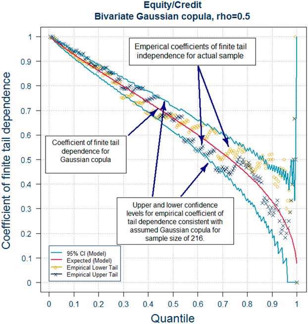
Figure 8 EQ/CR bivariate Gaussian coefficient=0.5
Note that the Gaussian and Student’s t copula are elliptic and therefore radially symmetric so that the model coefficients of finite tail dependence are equal; that is, λ L (q)=λ U (q) for all q.
3.8.4 Practical considerations
The approach assumes that the choice of copula has already been made and is used to adjust a best estimate view of the correlation parameters to make an allowance for tail dependence. Depending on the numbers of risk pairs involved, it may not be practical to assess each pair individually. It may therefore be desirable for practical reasons to perform the full analysis only for those pairs of risks where the sensitivity of the output to a defined change in the correlation assumption exceeds a certain threshold.
One option to further reduce the volume of detailed analysis required would be to fit a Student’s t copula to each risk pair and perform more detailed analysis if the fitted degrees of freedom parameters falls below a specified threshold.
A limitation of this approach is that it only considers conditional probabilities based on both risk factors simultaneously exceeding their q th percentile – that is, the percentile is identical for both risk factors. It therefore considers conditional probabilities only along a ray extending from the origin at an angle of 45° into the “north-east” and “south-west” quadrants. In order to ensure that the approach looks at the appropriate tail, it is necessary to consider the undertaking’s exposure to each risk pair (e.g. by consideration of the biting scenario). It may be necessary to adjust the data by multiplying one of the risk factors by (−1) in order to ensure that the analysis takes into account the direction of changes which are expected to bite.
3.8.5 Worked example
We illustrate the technique using our equity and credit spread (EQ/CR) data set. We assume that the undertaking’s exposure is to a fall in equity values combined with an increase in credit spreads. We have therefore multiplied equity returns by (−1) for the purposes of the analysis. As noted in section 3.5.4, the MPL fit for a bivariate Gaussian is given by ρ=0.488 and for bivariate Student’s t distribution is given by (ρ,υ)=(0.465,2.6). A potential initial candidate model may therefore be a Gaussian copula with correlation coefficient 50% (or −50% when we adjust back to our original coordinate system). This model is illustrated in Figure 8 which contains the following charts (Table 9).
Table 9 Additional Details for Figure 8

Figure 8 shows some asymmetry in the tail with the conditional probabilities associated with extreme upwards movements in credit spreads and falls in equity values somewhat higher than those corresponding to movements in the opposite direction.
The central solid line in Figure 8 tends towards zero. This is consistent with the Gaussian copula having a coefficient of tail dependence of zero.
The confidence intervals expand as events become more extreme, reflecting an increasing funnel of doubt as the volume of data in the tails decreases.
Although the circles of the lower tail do not appear inconsistent with the confidence intervals, they are at the boundary, particularly just below the 80th percentile and exceed the boundary around the 90th percentile. If a Gaussian copula is to be used, this may suggest use of a stronger correlation assumption if the SCR biting scenario includes percentiles of 80th or above in credit spreads and equity risk factors.
Figure 9 is similar but with the Gaussian copula model replaced by the bivariate Student’s t copula estimated using MPL techniques.
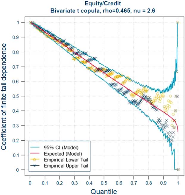
Figure 9 EQ/CR bivariate Student’s t ρ=0.465, nu=2.6
Comparing the two charts, it is apparent that the Student’s t copula produces greater values of conditional probabilities in the tail of the distribution and the solid central line no longer converges to a value of zero, consistent with a non-zero value for the coefficient of tail dependence.
The Student’s t copula appears consistent with the sample data across a wider range of percentiles – in particular, both in the extreme tail and in the body of the distribution.
If it has been decided to use a Gaussian copula model, then one may use a correlation assumption estimated from data using one of the techniques described in sections 3.5 and 3.6 to assist in informing one’s central view of an appropriate assumption. However, if analysis suggests that the biting scenario is likely to be in the tail of the distribution, then it may be considered appropriate, given the low degrees of freedom parameter for the fitted Student’s t copula, to make an adjustment to the correlation parameter to allow for tail dependence.
One approach would be to inspect various alternative parameter values – for example, by “flicking through” a set of graphics comparing the coefficients of finite tail dependence for the assumed parameterisation and the envelope of confidence intervals around it with the empirical coefficient of finite tail dependence. Figures 10 to 12 show how the coefficient of finite tail dependence changes as the correlation assumed in the Gaussian copula is strengthened in increments of 10 percentage points. The coefficients of finite tail dependence for the copula model, together with the envelope of confidence intervals, increase, allowing a judgement to be made on a parameter value which places the model output in an appropriate place relative to the empirical values.
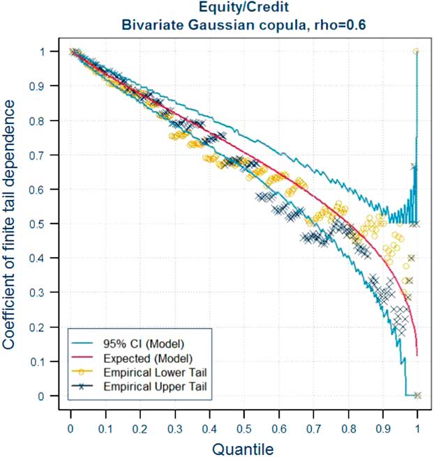
Figure 10 EQ/CR bivariate Gaussian coefficient=0.6
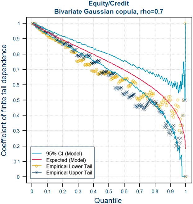
Figure 11 EQ/CR bivariate Gaussian coefficient=0.7

Figure 12 EQ/CR bivariate Gaussian coefficient=0.8
If one had a view on the percentiles underlying the SCR biting scenario, one could aim to use a correlation assumption which produced values of the coefficient of finite tail dependence which were broadly consistent with the empirical values in the neighbourhood of that percentile.
For example, if the biting scenario involved a combination of equity and credit spread stresses at around the 95th percentile, one might judge that a correlation assumption of 60% might undershoot the conditional probabilities suggested by the data whilst a correlation assumption of 80% might overshoot. A correlation assumption of 70% might be judged a reasonable compromise.
Alternatively, if there was a desire to retain a model with explicit tail dependence, one could use such plots to inform the choice of parameters. For example, Figure 13 illustrates one potential choice of parameters for a Student’s t copula which appears to more closely match the lower tail (depicted by circles).
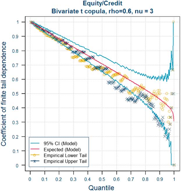
Figure 13 EQ/CR bivariate Student’s t ρ=0.6, nu=3
3.9 Correlation “Hardening”
The approach described in section 3.8 uses inspection to select an adjustment to the central view of a correlation of a Gaussian copula to obtain a level of conditional probabilities which is considered appropriate. An alternative approach to determine this “hardening” of the correlation assumption, which follows the same underlying concept, but reduces the level of judgement involves targeting of the conditional probability for a Gaussian to produce the same value as that for a Student’s t model with a given degrees of freedom parameter at a chosen percentile. This approach may be useful where one has calibrated a Student’s t copula for each pair of risks, for example, using the techniques of section 3.10, but where a decision has been to use a Gaussian copula. Instead of using graphical methods to select appropriate adjusted correlation parameters, the “hardening” adjustment is determined with the aid of look-up tables.
For each degrees of freedom parameter of a bivariate Student’s t copula, a look-up table is produced which shows for each correlation parameter of the t copula and each percentile, the correlation parameter of a bivariate Gaussian copula which produces the same joint exceedance probability at that percentile. It is straightforward to produce such tables using standard statistical packages such as R.
If one has a view of an appropriate percentile (e.g. based on knowledge of the biting scenario), a correlation parameter (or, equivalent, a “hardening” adjustment) for the Gaussian copula can then be read directly from the table.
By means of illustration, suppose we have determined that a Student’s t copula with 7 degrees of freedom is appropriate. Table 10 shows, for a given correlation parameter of the t copula, the correlation parameter of a Gaussian copula which is required to produce the same joint exceedance probability at various percentiles. Table 11 shows the same information but re-expressed as the amount (or “hardening”) that must be added to the correlation parameter of the t copula at each percentile to produce the equivalent correlation parameter of the Gaussian copula.
Table 10 Equivalent Gaussian Correlation Parameter

Table 11 Addition to Correlation Parameter of Student’s t Copula (“Hardening”)

For example, if one believed that the biting scenario was around a 95th percentile event in both risk factors and the correlation parameter of the t copula was +25.0%, one might opt to use a correlation parameter of 38% in the Gaussian copula (prior to any further adjustments based on expert judgement or for rounding or positive definiteness) (Figure 14).
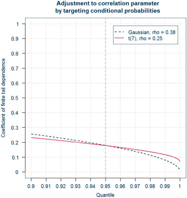
Figure 14 Hardening correlation parameter of a Gaussian copula by targeting conditional probability
According to the Towers Watson Limited (2015) Solvency II Pillar 1 Calibration Survey, companies using a Gaussian copula included the following margins over their best estimate correlation assumptions for market and non-market risks.
Table 12 shows that UK life insurers which use Gaussian copulas are making some significant adjustments to the correlation assumptions in order to allow for tail dependence. These adjustments may differ from one undertaking to another depending on their exposures to different risk factors and the judgements of their Boards. As we saw in the EQ/CR example of section 3.8.5, an undertaking with significant exposures to increases in credit spreads and falls in equity values may judge that it would be appropriate to strengthen the sample correlation assumption derived from its data by 20–30 percentage points in order to allow for tail dependence.
Table 12 Correlation “Hardening” Applied in Practice (Towers Watson Limited (2015) Solvency II Pillar Calibration Survey 2015)

3.10 Fitting Using Higher Order Rank Invariants
3.10.1 Background
Another approach to copula fitting – see Shaw et al. (Reference Shaw, Smith and Spivak2010) – is conceptually similar to a MoMs approach in that the parameters of the copula are selected so that certain higher order rank invariants of the model are equal to sample values derived from the data. Its main application currently is in the case where a Student’s t copula has been chosen for modelling and the correlation matrix and degrees of freedom parameter υ has to be selected, although the approach generalises to other copulas. Under the approach set out by Shaw et al. (Reference Shaw, Smith and Spivak2010), the correlation matrix and a degrees of freedom parameter υ are selected using an algorithm, which aims to produce a match between certain rank invariants of the model and their corresponding sample values. The two rank invariants are the Spearman’s rank correlation – a first-order rank statistic – and a higher order rank invariant called “arachnitude”. The latter statistic is so-named as it measures “off diagonal” dependencies that give rise to the “star” shape observed in some scatter plots of bivariate Student’s t copula or “spider’s legs” extending into the corners of the hypercube [0,1] d in higher dimensions.
The rank invariant “arachnitude” is defined in Smith & Sweeting (Reference Smith2011) as: ρ((2F X (X)−1)2, (2F Y (Y)−1)2), where ρ is Pearson’s (linear) correlation.
The equivalent sample statistic is given by the formula:
 $${\rm arachnitude}\, \, {\equals}\, \, {{45} \over {4N\left( {N^{2} {\minus}1} \right)\left( {N^{2} {\minus}4} \right)}}\left[ {\mathop \sum\limits_{k\, \, {\equals}\, \, 1}^N \left( {2R_{k} {\minus}N{\minus}1} \right)^{2} \left( {2S_{k} {\minus}N{\minus}1} \right)^{2} {\minus}{{N\left( {N^{2} {\minus}1} \right)^{2} } \over 9}} \right]$$
where the {R i } and {S j } are the ranks of the sample data {x i } and {y j } (Smith, 2014). Arachnitude takes values between −1 and 1 and is large when extreme high or low values of X tend to coincide with extreme high or low values of Y. It is therefore a measure of dependency along both diagonals rather than just along the 45° line as in the case of tail dependence.
A summary of the theoretical basis underlying the approach is provided in Appendix A.3. An outline of the calibration approach is provided in section 3.10.2.
3.10.2 Parameter selection algorithm
In practice, the copula we wish to parameterise will relate to a d-dimensional distribution (where d≥2) such as a set of market risks. We therefore have to solve for d(d−1)/2+1 parameters (correlation parameters for d(d−1)/2 pairs of risk factors and 1 degrees of freedom parameter). The degrees of freedom parameter is common to all pairs of risk factors, which acts as a constraint on the system of equations. This means that in practice it is not possible for all combinations of (rank correlation, arachnitude) pairs to be “reached” simultaneously by the parameters of a Student’s t copula.
The most commonly used approach to solving this constrained system of equations is as follows:
-
(A) Produce a two-dimensional scatter plot showing the sample values of (rank correlation, arachnitude) for each risk pair.
-
(B) Generate a one-dimensional family of curves (parameterised by a single degrees of freedom parameter), for which each curve describes arachnitude as a function of rank correlation, using the following algorithm:
-
(i) Fix a grid of correlation parameters and a grid of degrees of freedom parameters for a bivariate Student’s t copula;
-
(ii) For each degrees of freedom parameter υ:
-
(a) Select a copula correlation parameter ρ from the grid and generate a set of simulated values from the bivariate Student’s t copula with parameters ρ and υ.
-
(b) Calculate the rank correlation and arachnitude for this set of simulations and plot it.
-
(c) Loop back to step (a) and select the next correlation parameter from the grid.
-
(d) Repeat until all copula correlation parameters have been used.
-
-
(iii) Draw a curve through the plotted (rank correlation, arachnitude) pairs for the given value of υ.
-
(iv) Repeat (ii) and (iii) for each υ in the grid.
-
-
(C) The algorithm of step (B) generates a one-dimensional family of curves parameterised by υ showing the relationship between arachnitude and Spearman’s rank correlation. Use judgement to choose a value of υ such that an appropriate balance is obtained between the number of sample values of (rank correlation, arachnitude) that lie above the corresponding curve and the number that lie below.
-
(D) The judgement at step (C) could take into account exposures to each risk. For example, υ could be chosen so that the resulting curve was closer to those points corresponding to risks for which exposures were significant.
-
(E) This fixes a degrees of freedom parameter υ for the d-dimensional Student’s t copula, which is common to each risk pair. For each pair of risk factors, back solve for the correlation parameter of the bivariate Student’s t copula with degrees of freedom parameter υ which gives the corresponding Spearman’s rank correlation on the fitted curve (i.e. solve for the correlation parameter which produces the (rank correlation, arachnitude) pair resulting from “dropping” the sample (rank correlation, arachnitude) vertically onto the fitted curve). As the relationship of equation (1) is exact only for a Gaussian copula, the back solving involves numerical techniques (e.g. linear interpolation using the grid created in Step B(i)).
-
(F) Adjust the correlation matrix obtained in step (E) to make it PSD (e.g. using one of the techniques described in section 3.14).
The approach is illustrated in Figure 15 which is reproduced from Shaw et al. (Reference Shaw, Smith and Spivak2010). The example is based on monthly total returns for equity indices of 18 different geographies (i.e. 153 distinct pairs of risk factors) over the period 31 December 1969 to 31 December 2009 and shows curves of (rank correlation, arachnitude) for a constant correlation matrix and varying degrees of freedom parameter υ. For this particular data set, it would appear that υ=5 provides a reasonable balance between data points that lie above and below the curve. However, a different choice may be appropriate if exposures are significantly weighted towards a subset of the risks.
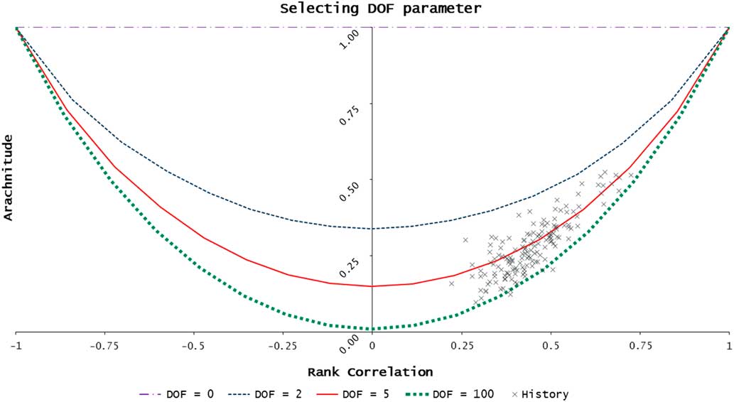
Figure 15 Monthly total returns for equity indices of 18 different geographies (i.e. 153 distinct pairs of risk factors) over the period 31 December 1969 to 31 December 2009 (reproduced from Shaw et al., Reference Shaw, Smith and Spivak2010 with permission)
An alternative approach to parameterisation modifies the approach described in this section by fixing the copula correlation matrix at the first (rather than final) stage in the process. This could be done, for example, by using the relationship of equation (2) involving Kendall’s τ which is exact for an elliptic copula such as a Student’s t. The resulting matrix is then made PSD, if required. With the copula correlation matrix fixed, one can then produce a family of (rank correlation, arachnitude) curves parameterised by the degrees of freedom parameter υ using the techniques described in Step B(ii) and select an appropriate value for υ as in Step (C).
3.11 Strengths and Limitations of Calibration Techniques
The Table 13 provides a comparison of the strengths and limitations of some of the techniques for informing the parameterisation of copulas discussed in this paper. Ultimately it is a question of judgement, taking into account the choice of copula, as to which method is most appropriate.
Table 13 Comparison of Calibration Techniques

MPL, maximum pseudo-likelihood.
3.12 Expert Judgement Overlay
Copula parameters cannot in practice be selected based solely on an analysis of data due to factors such as:
-
(i) The period of data available for some risk pairs may be very short and not contain sufficient data on extreme events or be dominated by behaviour which may not fully reflect expected future relationships (see section 3.6).
-
(ii) Analysis of different risk factor pairs over different periods of time may lead to inconsistencies between assumptions (see section 3.14).
It is therefore essential to take into account other factors such as those discussed in section 3.13 to assess whether the values suggested by the data are appropriate and to apply expert judgement to adjust those values, if appropriate.
3.13 Assumptions Where Data are Scarce or non-Existent
The techniques described in sections 3.8–3.10 may be useful in informing the selection of an assumption where there is a reasonable volume of relevant data. In practice, this means that they are useful only for certain market risks and, even then, it is still necessary to apply expert judgement to assess whether the assumptions are reasonable and adjust them where appropriate. For other types of risk, the selection of an assumption is necessarily based on expert judgement alone. In this section, we provide a summary of some of the factors which should be considered (i) when selecting correlation assumptions where there is little or no relevant data available; or (ii) where data are available, assessing the reasonableness of the assumption suggested by that data and using expert judgement to make adjustments where appropriate.
Factors which may be taken into account when selecting such assumptions include:
Causal relationships
Does a change in one risk factor have a tendency to result in a change in the other (or vice versa)? By what mechanisms does a change in one risk factor lead to a change in the other. How strong is that relationship? Note that a correlation between changes in two risk factor does not necessarily arise due to a causal relationship between the two risk factors, but can also arise because the values of both risk factors are influenced by a common underlying risk factor.
Common underlying risk factors
An association or correlation between increases in one risk factor and increase in another risk factor does not necessarily arise due to a direct causal relationship – see for example, section 6.1 of Shaw et al. (Reference Shaw, Smith and Spivak2011). For example, there may be a common underlying risk factor that has a tendency to “drive” simultaneous changes in two or more of the modelled risk factors. A large change in this common risk factor may tend to give rise to larger changes simultaneously in two or more of the larger risk factors. This is the case, for example, for the Student’s t copula, which is an example of a “Normal mixing distribution”. Under one representation of this copula, simulated values from a Gaussian copula are scaled by an independent (inverse Gamma) risk factor. This scaling by a common risk factor leads to a greater tendency for large values of the risk factors to occur simultaneously and the introduction of tail dependence. See for example, algorithm 6.10 of McNeil et al. (Reference McNeil, Frey and Embrechts2015) or algorithm 5.2 of Embrechts et al. (2003).
Tail dependence
Would one expect the relationship between changes in two risk factors to become less diffuse in the tails resulting in a greater alignment between the ranks of changes in one risk factor and the other? Here it may be useful to imagine the relationship in terms of scatter plots and the extent to which any clustering of extreme values could be expected.
Financial significance
How sensitive are the outputs of the model to changes in the assumption? This may have implications for the extent of any prudence which is considered appropriate to reflect uncertainty, the level of detail of the analysis and associated documentation and governance.
The above may assist in forming a view about the level of any correlation and the extent of any further allowance to be made for tail dependence. The extent of any additional allowance for tail dependence may also be informed by the amounts of any allowances made in calibrations for market risk factors (e.g. resulting from the approaches described in sections 3.8 and 3.9).
As for all areas of expert judgement, it is important to set out clearly the rationale for the assumptions, what a plausible range for alternative but nonetheless valid alternative assumptions might look like, the sensitivity of the model output under these alternative assumptions and the limitations relating to the expert judgements. A robust governance process should be followed. It may be useful for the governance to involve a number of experts from different areas of the business to ensure that, overall, the assumptions are coherent. The assumptions should also be subject to independent validation by personnel not involved in the process of their selection – see section 3.15.
The paper by Ashcroft et al. (Reference Ashcroft, Austin, Barnes, MacDonald, Makin, Morgan, Taylor and Scolley2016) provides some suggestions on the process of eliciting expert judgement and its validation.
The PRA has discussed the judgements used in setting its Quantitative Indicators for dependencies in two executive director updates dated 9 March 2015 (PRA, 2015a) and 15 January 2016 (PRA, 2016).
3.14 Internal Consistency and positive semi-definiteness (PSD)
3.14.1 Background
All valid correlation matrices satisfy an internal consistency condition known as “PSD”. Broadly speaking this means the correlations between all possible n-tuples of correlations are consistent. For example, if the correlation between risk pairs (X, Y) and risk pairs (Y, Z) are large and positive, one would expect the correlation between pair (X, Z) to be large and positive – see appendix A2 of Shaw et al. (Reference Shaw, Smith and Spivak2011), for more details.
Mathematically, this means that the eigenvalues of the matrix must all be non-negative. The correlation matrix approach applies a formula and will always produce a result when applied to the vector of capital requirements corresponding to each of the individual risk factors. However, if the correlation matrix is not PSD, the “sum of squares” approach will produce a zero or negative result when applied to certain capital vectors.
(Note that some copula simulation algorithms such as those based on the Cholesky decomposition as described in algorithm 6.10 of McNeil et al. (Reference McNeil, Frey and Embrechts2015) will only work if the matrix is strictly positive-definite. This is a stronger condition and requires all the eigenvalues to be strictly positive, or, equivalently that the matrix be PSD and all its columns are linearly independent. If the correlation is not strictly positive-definitive, then an alternative to the Cholesky decomposition must be used for simulating; e.g. techniques based on the decomposition of the correlation matrix in terms of a diagonal matrix of eigenvalues and an orthogonal matrix of eigenvectors.)
Correlation matrices derived from a multivariate data set where all risks are sampled over an identical period of time at coincident dates will always be PSD by construction. In the context of life assurance, this is unlikely to be the case for the following reasons:
-
∙ Where data are available, the period of time over which it is available for all the risk factors under consideration is likely to be very short. This results in the selection of assumptions on a pair-wise basis in order to maximise the use of the relevant data for each pair of risk factors.
-
∙ Use of judgement in the selection of assumptions, particularly where there is very scant or no relevant data.
-
∙ Possible inclusion of additional allowances for tail dependence.
-
∙ Any rounding convention applied when selecting correlations.
-
∙ Any further adjustments which may have been made (e.g. if the assumption suggested by the data are not considered to reflect the future relationship).
3.14.2 Adjustments
The initial candidate matrix may therefore not be PSD and so requires adjustment prior to use. There are several techniques available which vary in complexity. One of the more straightforward techniques involves elimination of negative eigenvalues. The candidate matrix is first diagonalised using standard eigen-decomposition techniques of linear algebra. Any negative or zero eigenvalues appearing along the diagonal of the diagonal matrix of eigenvalues are replaced by a small positive value chosen by judgement. The resulting matrix is then transformed back to the original coordinate system and the diagonal entries adjusted so they are all equal to one. This process is described in more detail in algorithm 7.57 of McNeil et al. (Reference McNeil, Frey and Embrechts2015).
More sophisticated techniques which seek to find the PSD correlation matrix which is in some sense “nearest” to the initial candidate matrix are also available. These techniques can be modified to apply weights to particular columns and rows, which may be useful if one has strong views that those assumptions are appropriate, or constrain an existing PSD sub-matrix to remain unchanged. See for example, Higham (Reference Higham2013).
3.14.3 Validation
Whichever technique for “PSD-ing” is used, users will need to be satisfied that the resulting matrix remains consistent with the views reflected in the selection of the “raw” candidate matrix originally approved. One may do this by inspection or introduce a process based on quantitative acceptance criteria. For example, one may inspect a histogram of percentage point increases in correlations or require that a specified proportion of changes fall within certain limits. However, a process based solely on changes to correlation assumptions does not take into account the implications for capital requirements. One may be willing to accept a larger movement in a correlation assumption between two insignificant risk factors that has a relatively small impact on capital requirements. One could therefore require that the effect of changes on capital requirements produced by a correlation matrix approach did not exceed a certain monetary limit. (The correlation matrix approach is used as the formula still produces a result even if the original matrix is not PSD.)
If the adjusted matrix does not meet the specified acceptance criteria, one may then have to: (i) seek approval to apply the adjusted matrix; (ii) use a more sophisticated adjustment technique, which may not be a practical option in the time available; or (iii) find an alternative set of adjustments by inspection, which may require a number of iterations. Failure to produce a suitable PSD matrix may indicate a more fundamental inconsistency within the original candidate matrix which requires more detailed investigation. It is therefore preferable to perform any adjustments necessary outside the production cycle, for example, as part of the calibration process.
3.15 Top-Down Validation Tests
Having chosen a copula model (e.g. Gaussian or Student’s t), selection of the parameters is generally a bottom-up process. However, it is important that consideration is given as to whether the resulting assumptions are collectively reasonable and appropriate for the purposes for which they are used. Some examples of top-down validation tools are provided below.
3.15.1 Peer review
It is good practice for the proposed assumptions to be subject to review by one or more individuals with relevant expertise from around the business. Meetings could be held with the purpose to review and challenge proposals. These meetings could examine the rationale for particular assumptions, perhaps identifying relationships between changes in risk factors which had not been fully considered or whether conclusions drawn from analysis of data were reasonable or required further adjustment. The review should also consider whether the assumptions were appropriate on a prospective basis and were not unduly driven by historical data, taking into account the scarcity of data, the uncertainty in the analysis and expectations regarding the future relationship between changes in risk factors.
3.15.2 Independent review
To mitigate the risk of recommendations made by individuals or an expert judgement panel such as that described in 3.15.1 becoming biased by a desire for consensus and dismissing alternative views (“groupthink”), it is good practice for proposals to be reviewed by individuals who are independent from the formulation of the original proposals and subject to a different reporting line. The idea behind this is that the reviewers should be free of any influence from those responsible for development of the model, which, in theory, should lead to a more objective review. The Internal Model requirements of Solvency II require such an independent validation process. In some cases, the Board may wish to seek additional assurance through an external review of some or all of the assumptions, particularly those which are material.
3.15.3 Sensitivity testing
Assumption sets underlying the dependency structures used in life company internal models typically have high dimensions. For example, if there are 25 risk factors, the correlation matrix underlying a Gaussian copula will have 300 distinct parameters.Footnote 2 The Towers Watson Limited (2015) Risk Calibration Survey indicates that some firms use up to 10,000 correlation parameters. In testing assumptions, it is important to focus on those which have the most significant impact on the model output. These can be identified by testing sensitivities to individual assumptions. In general, a correlation matrix approach may be adequate in ranking assumptions for this purpose rather than re-running the full copula + proxy model simulation many times.
When testing sensitivities, one should have regard to the relationships between changes in risk factors. For example, strengthening the correlation between risk factors X and Y may suggest strengthening other correlations involving X or Y for reasons of maintaining internal consistency. A sensitivity to a change in one correlation in isolation may not give a reasonable view of the total change if one were to make corresponding changes in all related assumptions.
3.15.4 Scenario analysis
This involves showing stakeholders the type of real-life situation which could give rise to losses of a magnitude similar to the SCR and asking them to form a view on whether that scenario is reasonable, given their knowledge of risk profile of the business. Any unexpected features of the scenario could indicate an inappropriate choice of parameters and trigger further investigation.
For example, one could examine scenarios which, when ranked by losses, lie in a “window” around the scenario corresponding to the SCR. Alternatively, one could average out the scenarios in the window, perhaps using kernel smoothing techniques which apply different weights to each scenario, to determine a “smoothed average” or “biting” scenario which is representative of the scenarios giving rise to losses equal to the SCR. That scenario could then be expressed in terms of the corresponding changes in risk factors which would be meaningful to stakeholders; for example, a fall in equity values by x%, a reduction in the level of interest rates of y basis points at term t; an increase in credit spreads on A rated corporate bonds of z basis points, an improvement in life expectancy of males aged 65 of w years, etc.
One could then invite stakeholders to assess whether a scenario was reasonable. For example, if a risk factor to which the business had a significant exposure featured relatively weakly in the biting scenario, this could prompt questions about whether the strength of the associations between that risk factor and others was appropriate. Alternatively, if a certain risk factor featured relatively strongly in the scenario(s), is that result reasonable given exposure to this risk factor and expectations of stakeholders regarding the strength of its relationship with other risk factors?
Conversely, one could ask stakeholders to postulate a scenario involving simultaneous changes in several risk factors, evaluate the “heavy” or proxy model on that scenario and determine its corresponding ranking or percentile in the overall distribution of losses. One could then ask stakeholders to form a view on whether the ranking of that particular scenario seemed reasonable.
In practice, it may be very challenging to ask stakeholders to assign a probability to losses under a particular scenario. However, presenting scenarios in terms of “real world” changes in risk factor values which are meaningful to the stakeholders such as falls in equity values, increases in interest rates or changes in persistency rates can make the calculations feel more “real”, help engage stakeholders in discussing the relationships between risks and provide a high level sense check on the results. Indeed, the ability of a simulation-based approach to identify a range of scenarios giving losses of magnitude comparable to the SCR is one of the main advantages of this approach compared to the correlation matrix approach.
3.15.5 Industry benchmarking
Several actuarial consultancies produce annual surveys comparing practices, models and calibrations. The validity of analyses based on survey results will necessarily be subject to limitations as they may not always compare “like with like”. For example, companies do not all adopt identical definitions of all risk factors, which may lead to different calibrations for models describing changes in similarly named risk factors or different correlation assumptions. Companies with insignificant exposures to a given risk factor may find it proportionate to adopt strong assumptions for correlations between that risk factor and other risk factors rather than spend resource on detailed analysis, whereas companies with more significant exposures may prefer to perform a more detailed analysis in order to avoid excessive prudence. The actual copula model used may also differ between one company and another. A correlation assumption adopted by a company using a Student’s t copula may not be directly comparable with the corresponding assumption of a company using a Gaussian copula, particularly if the latter has chosen to adjust the assumption to make an allowance for tail dependence.
Nevertheless, comparisons based on surveys can be useful in highlighting any assumptions which appear out of line and help focus validation effort on the rationale for those assumptions.
3.16 Selection of the Copula
We discuss briefly the validation of the choice of copula. Due to the uncertainties arising from lack of relevant data and modelling constraints, the selection of a copula model is likely to be driven by practical considerations such as the use test and prior beliefs, with appropriate adjustments made to the parameters to allow for the limitations of the chosen model.
The scarcity and, in some cases, absence of relevant data necessarily limits the extent to which standard statistical tests may be applied in practice. Nevertheless, one may consider it appropriate, if only to demonstrate compliance with the statistical quality standards of Solvency II, to perform some tests to validate the choice of copula model. Such tests fall into two broad categories:
3.16.1 Goodness of fit tests
For example, the Table 14 provides a list of copula models with some potential tests and further references.
Table 14 Copula Models and Potential Tests

The first three tests are restricted to a specific family of copula: the Gaussian or Student’s t. They each involve “dimensional reduction” by condensing the information included in the data into values of one or two one-dimensional test statistics whose p-values are then generated assuming the null hypothesis.
The version of Mardia’s test involves first converting the empirical copula into a test observation from a multivariate Normal by applying the inverse distribution functions of a standard Normal distribution to each marginal of the copula.
The tests of Malevergne and Sornette are based around the squared Mahalanobis distance for each observation in the sample. A variety of test statistics based on the usual Kolmogorov–Smirnov or Anderson–Darling statistics may be defined and their empirical distributions derived by bootstrapping assuming the null hypothesis of the Gaussian copula holds.
The test of Kole, Koedijk and Verbeek extends that of Malevergne and Sornette to a Student’s t copula through a modification of the Mahalanobis distance.
The “blanket” tests of Genest, Rémillard and Beaudoin are so named because they can be applied to any family of copula. Instead of using an intermediate statistic to reduce the dimension, the test statistic is generated directly from the empirical copula. Again, various forms of the test statistic may be used, the most common being the Cramér von Mises statistic which is a measure of the L 2 distance between the empirical copula and hypothesised copula. The distribution of the test statistic and p-values must be generated using bootstrapping techniques. Test functions are available in the “copula” package of R.
3.16.2 Model filters
These provide a method for assessing the appropriateness of using a more complex model with additional parameters. For example:
-
(i) Likelihood ratio tests for nested models.
-
(ii) Penalised likelihood functions such as Akaike information criteria (AIC), Bayesian information criteria (BIC) or other information criteria.
3.16.3 Usefulness of tests in practices
In practice, in a life insurance context, a meaningful analysis is possible only for a subset of market risks. Even then, the results of the tests are inconclusive – see for example, Makin & Stevenson (Reference Makin and Stevenson2014). It is possible that such tests may have greater power when applied to larger (and more homogeneous) sample sets such as monthly returns on equity indices for different geographies. However, for the relatively small data sets which are most often used in a life insurance context, we have found that such tests provide little useful additional insight.
We have also found when comparing two versions of the blanket tests to our sample data (the standard Cramer von Mises test and the Cramer von Mises test with the Rosenblatt transform – see Genest et al., Reference Genest and Rivest2009), that the “stronger” version of the test based on the Rosenblatt transformed resulted in non-rejection of both the Gaussian and Student’s t model whereas the standard version of the test resulted in rejection. We believe this may be due to limitations in deriving the bootstrapped distribution function of the test statistic when applied to small samples.
4 Proxy Models – Design, Validation and Communication of Results
4.1 Overview
In section 1.1 of this paper we outlined some of the drivers for developing more sophisticated capital models, and in particular those that use a copula-based simulation approach. This enables firms to generate a rich and complete distribution of profit and loss, which can inform regulatory and economic capital requirements, and assist firms to understand the nature of the risks that they face and their impact on the balance sheet.
However, such simulation techniques are only useful if we can, with reasonable accuracy, calculate the financial impacts on an insurer’s balance sheet over a wide and rich set of points. For example, for a credible distribution of profit and loss, firms would expect to run hundreds of thousands, or even millions of samples from the copula distribution. In most cases, current technology prohibits firms from running heavy models at all of the required simulation points. Because of this, many firms have developed “proxy” models, which are used to estimate the relevant financial metrics, such as movement in surplus.
The technical grounding of this topic was discussed in some detail by Hursey et al. (Reference Hursey and Scott2014), while in this paper we address more practical issues such as the choices involved when designing and fitting a proxy model. We then discuss validating and communicating the results of proxy models.
In this section, we provide a brief overview of proxy modelling and highlight some of the challenges practitioners have in communicating their results to senior management and other stakeholders. We then consider the design, fitting and validation of proxy models, including a discussion of options available to a firm in the event its proxy model does not meet its target validation thresholds. Finally, we return to consider the communication challenges, and how these can be addressed.
4.2 Background
As we mentioned above, development of proxy models was initially motivated by the need to calculate a balance sheet quickly, partnering copulas in a simulation-based approach to calculating capital requirements. These techniques therefore have the aim of being able to estimate financial values connected to insurance liabilities without needing to perform full heavy model runs. This has led to their expansion into other applications, such as solvency monitoring, where a firm can use its proxy model to calculate the impact on its balance sheet of market movements and movements in other risk factors, as well as the allowing for new business and run-off of existing business.
The two most common types of proxy models are proxy functions and replicating portfolios:
-
∙ Proxy functions – this is a general technique where the user runs a number of fitting scenarios which are used to express the determinant variable (e.g. profit/loss or asset/liability value) as a function of one or more explanatory variables (commonly referred to as risk factors). This is often performed using regression techniques or by interpolating between fitting scenarios.
-
∙ Replicating portfolios – this technique aims to use hypothetical portfolios of assets (or more general financial instruments) to replicate the value of the firm’s liabilities and how they move in relation to various risk factors. The financial instruments need not be real in the sense that they are traded in real markets, that is, they could be synthetic. If the replicating financial instruments can be valued analytically, then the liabilities can be easily and quickly valued under a wide range of scenarios.
Whilst these two methods are different in their construct, they both adopt the same principle of representing movements in the insurer’s balance sheet in terms of a set of simplified basis functions. In fact, replicating portfolios could be seen as a special case of a proxy function, as ultimately with this approach we are trying to derive an analytical formula to estimate asset and liability values.
In the remainder of this section we focus on proxy functions, as these are the dominant technique adopted in industry. However, much of our discussion on the design of proxy models, and of the communication and validation of their results is also relevant to users of replicating portfolios.
As an example, Figure 16 shows a hypothetical proxy function showing the movement of an exposure to equity values risk. Here the function fitted is a degree 2 polynomial. In this case, we see that the firm incurs a loss on that particular line of business when equity values fall. We return to this example in subsequent sections.
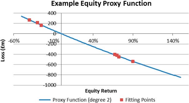
Figure 16 Example equity risk proxy function
4.3 Communication Challenges
In the past, senior management at insurance firms will have been aware that actuaries have developed and maintained large calculation models for valuing insurance liabilities. Governance frameworks and standards will have been established to demonstrate to the Board that the models are appropriate for use in producing financial statements and solvency assessments, for pricing new products, and for forecasting revenue and capital. These models will have been through thorough testing to validate that the models produce results that are consistent with the features of insurance products. Ultimately it is important that enough information be given to the Board so they can get comfort over the appropriateness of model usage and their limitations.
Table 15 lists challenges for communicating the use and appropriateness of proxy models to senior management.
Table 15 Communication Challenges in Proxy Modelling

4.4 Proxy Model Design
Although proxy models could be viewed as a simplistic tool, in reality firms need to design their calculation software to fit with its reporting needs and the specific structure of the organisation. A proxy model that is well designed will be able to produce many of the outputs that a firm needs. For example, economic capital can be calculated at various levels of the organisation’s hierarchy, and the capital can be allocated lower down if required to individual products or groups of products. Figure 17 illustrates a generic model structure. It shows different levels at which proxy functions could be established, and each level at which the firm could calculate profits or losses and would therefore capture diversification between risks at that level.
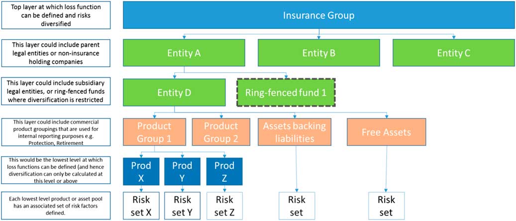
Figure 17 Proxy model design
The design of the model will be different between firms, and even within the same firm there could be more than one design to fit different purposes. Ideally, however, the firm would try to establish a single model that fits all of its reporting purposes but in the end this may not be achievable.
4.4.1 Design considerations
In the following sub-sections we identify questions that a firm designing its proxy model would consider. For each, we outline some of the factors that a firm could take into account when answering these questions.
4.4.1.1 What metrics does the model need to calculate?
The metrics on which a firm needs to report, both internally and externally, will affect the design of the model.
It is likely that the proxy model will be used to calculate the SCR, and it may also be used for an approximate roll-forward calculation in order to demonstrate continuous solvency monitoring. This can impact the hierarchical design of the model, and the level of granularity at which results are required.
There will also be internal reporting requirements, for example, VARs at certain confidence levels for risk appetite monitoring, or deep tail stresses for capital buffer setting. Again, this may impact the granularity required of the model if we are looking to assess results for different products or legal entities.
Does the company need to report on the assets and liabilities separately, or can it combine them in some or all circumstances? Separate asset reporting may be instructive, for example, in measuring and managing the risk of a credit portfolio. For many purposes we may be able to combine assets and liabilities, to the extent that we are able to fit curves adequately.
4.4.1.2 What is the structure of the company on which we are reporting?
The company structure, as illustrated in Figure 17, will have a large influence on the design. Firms will usually need to report results externally at legal entity level, and for designated Insurance Groups. However, firms may also want to report results at other internal layers, for example, by geography or for certain holding companies.
Firms may also be required to perform calculations at sub-fund level. For example, under Solvency II, most with-profits funds and all matching adjustment portfolios are treated as if they were ring-fenced funds, where the nature of the fund results in restrictions on the ability of capital resources to absorb losses arising in other parts of the business. The aggregation model must then be set up to be able to calculate results for those separate portfolios and reflect the restrictions on loss absorbing capability.
Finally, firms may have defined business units or product groups at which they manage the business commercially. This may necessitate output at that level of granularity. However, the greater the level of granularity, the more proxy functions that will need to be fitted and validated. Whilst granularity is required to the extent that homogenous assets and liabilities will be easier to fit adequately, too much will require excessive fitting and validation. There may be more approximate ways to allocate results down to more granular products, for example, defining easily accessible risk drivers to approximate the exposure to risk.
Generally, a firm will place Groups or Legal Entities at the top of the structure and more granular categories at the bottom, for example, products or asset portfolios. It will be necessary to fit proxy functions at the lowest level of the hierarchy in order to produce results for that level.
4.4.1.3 For what other features do we need to account?
There will be other, more idiosyncratic, features of a firm that need to be reflected in models of its balance sheet, such as:
-
∙ Tax;
-
∙ Fungibility restrictions;
-
∙ Reinsurance;
-
∙ Management actions;
-
∙ Complex risks, such as operational risk.
It will be up to an individual firm to determine appropriate methodology for these modelling features, taking into account their materiality. In particular, it may decide to allow for them explicitly in the design of the proxy model. However, it may be more appropriate to fit proxy functions to exposures net of these features, or to allow for as an adjustment to the result produced by the proxy model.
4.4.2 Summary of proxy model design
The above considerations will influence the design of the proxy model. In summary, a firm designing its proxy model will need to decide:
-
∙ The hierarchical structure of the model, which will determine at what levels we may be able to simulate and order losses and thus calculate diversified results.
-
∙ The lowest level of the hierarchy at which proxy functions are fitted. This sets the most granular level at which results can be analysed (e.g. product groups, legal entities).
-
∙ How to reflect any constraints to the diversification that can be achieved, for example, due to ring-fencing restrictions.
-
∙ Where and how the tax impacts on profits and losses can be calculated.
-
∙ The risk factors to be used in the model, and to which products/entities these apply.
Where firms are using third party software supplied by an external vendor, there may be constraints imposed by that software, for example, a limited range of mathematical functions (as well as statistical distributions and copulas) that can be used. However, a firm will still need to ensure that the proxy model provides a materially accurate representation of their business.
Note that the above design decisions have not yet considered the methodology for fitting proxy functions. We discuss this in the next section.
4.5 Proxy Model Fitting
4.5.1 Objectives for model fitting
We now consider the choices around how to fit the model. First, we define a possible range of objectives of the fitting process.
-
∙ Well fitted: The model must fit the firm’s heavy models well, over an appropriately wide range of scenarios. This may focus on achieving strong fit at particular points or scenarios, for example, around the 99.5th percentile value at risk (VaR) to meet SCRs, or at other points as used by the business for risk measurement. However, it is a requirement of Solvency II that firms produce a full Probability Distribution Forecast so it will be necessary to achieve a strong fit across a range of quantiles. Testing of this accuracy objective is part of the model validation process.
-
∙ Parsimonious: The model should not be more complicated than is necessary. The fitting approach should not lead us to implement proxy functions that are more complex than is required. For example, higher order polynomial coefficients and joint terms should only be included if they materially improve the fit of the model. Testing of the parsimony objective is inherent in some mathematical fitting approaches – for example, AIC or Bayes’ information criterion (section 4.5.3). Some firms use a bespoke information criterion to select the model. If firms are using expert judgement to determine the structural form of the proxy functions, it would be more difficult to prove the satisfaction of this objective.
-
∙ Avoid over-fitting: This would normally be defined as an approach that overly focusses on fitting to the sample observations. In applications where observations include large statistically random errors, this means over-fitting to those errors (i.e. fitting to the “noise” rather than the “signal” in the data). This is less likely to be relevant in insurance applications, where the asset and liability calculations are either deterministic or based on stochastic models with sufficiently many simulations to ensure convergence. However, over-fitting in the context of proxy models would mean placing too much emphasis on achieving an accurate fit in the areas that the fitting runs are performed. Further, over-fitting can lead to results in the tails of the distribution that are not sensible due to turning points in the proxy function that occur just outside the fitting range. The range of scenarios over which the proxy model is valid should be clearly specified as a limitation and a trigger framework produced so that the curve fitting process is repeated where necessary. Graphical validation can provide a quick and instructive view of the curves that are fitted (at least up to three dimensions) so that the behaviour can be sense checked. Charts illustrating the use of graphical validation for this purpose are included in section 4.6.3.
-
∙ Practical: The fitting process also needs to lead to practical proxy functions which satisfy any constraints imposed by the simulation software used and can therefore be incorporated into the firm’s simulation model. This may preclude certain functional forms or polynomial orders.
4.5.2 Choice of proxy function form
Whilst the coefficients are a result of the proxy function fitting, the functional form itself is influenced by the approach taken to curve fitting.
For example, the functional form for a univariate proxy function may consist of the following basis functions:
-
∙ Polynomials up to a particular order (x, x 2, x 3, …)
-
∙ Another function, such as the exponential function.
The general form of this proxy function, p(x), which explains balance sheet movements under changes in risk factor x, is as follows:
 $$p\left( x \right)\, {\equals}\, a_{1} x{\plus}a_{2} x^{2} {\plus}a_{3} x^{3} {\plus}\,\ldots\,{\plus}be^{x} $$
Interaction terms can be allowed for similarly, through polynomials or other functions in two or more risks.
Approaches to choosing functional form can be categorised according to whether they are theory driven or data driven.
Adopting a theory-driven approach would mean using the firm’s knowledge about its assets and liabilities, and its exposure to risk factors to determine the functional form of the model, or at least to restrict the number of possible coefficients of the model through expert judgement. For example, there may be an economic theory or business intuition that the impact of a particular risk factor on a particular metric will be linear.
The other extreme is a data-driven approach, which would be to run a very large range of stresses in the heavy models and use mathematical techniques to reduce the proxy functions down to a suitable form. This approach could start with a very large number of possible terms, and the aim of the mathematical technique would be to gradually reduce the proxy functions whilst maintaining an adequate level of fit. Alternatively, it could build up the model adding one term at a time. An example of such a technique is stepwise regression, which is described in section 4.5.3.2.
A firm will need to decide the most appropriate method for selecting its proxy function forms and should justify and record why it believes the chosen approach is appropriate (as well as what alternatives were considered and why these were judged to be less appropriate). It may also be possible to perform the form selection exercise off-cycle (out of the production period), if the exposures modelled are stable over time.
4.5.3 Fitting tools
In this sub-section, we provide an overview of some methods that can be used to fit proxy functions.
4.5.3.1 Regression methods
A common method to fit proxy functions in practice is ordinary least squares (OLS) regression (due to its simplicity, age and estimates having strong statistical properties). For a given formulaic structure, this method chooses the coefficients of proxy function which minimise the sum of squared errors (SSEs) relative to the results of heavy models evaluated at fitting scenarios. As a variant, firms may wish to use a weighted least squares approach, which applies a weighting function to the regression to put more/less weight on different parts of the fit.
Hursey et al. (Reference Hursey and Scott2014) provide formulaic detail on these methods, and this is not repeated here.
4.5.3.2 Stepwise regression
A common mathematical technique used to determine which terms to include in a regression model is stepwise regression. In the context of proxy modelling, it can be used to determine the form of the proxy function. The aim of this technique is to step through different possible forms of the proxy function – adding or removing one term (or cross-term) at a time – and assess the fit at each level according to some pre-defined statistical criterion. The steps can either start at a very basic model then build up additional terms, or vice versa. The stepping through can be automated computationally and so implicitly allows the firm to consider a very large range of possible model calibrations and automatically choose the most appropriate based on that statistical criteria.
Different statistical criteria exist for use in a stepwise regression. The most commonly used in actuarial models are the AIC and BIC. These are both statistics that aim to assess the trade-off between the complexity of the model and its goodness of fit. See chapter 6 of James et al. (Reference James, Witten, Hastie and Tibshirani2015) for further details.
An alternative to information criteria is to run a set of out-of-sample (OOS) scenarios to discriminate between various possible structures in a stepwise regression scheme. These OOS runs would need to be independent of those to be used for validation (i.e. it requires additional modelling to be performed during the production cycle).
4.5.3.3 Alternative regression techniques
There are also alternative techniques, such as ridge regression and lasso regression, which apply a specified penalty function to the regression coefficients.
These techniques can result in an improvement in fit relative to OLS regression; lasso regression sets some coefficients to zero, thereby also selecting the form of proxy function. However, this can come with an associated increase in bias. For more information see, for example, James et al. (Reference James, Witten, Hastie and Tibshirani2015).
4.5.3.4 Polynomial interpolation
It is also possible to calibrate proxy functions by choosing a polynomial which interpolates between a set of fitting points. In this case, we would choose a polynomial of degree N to interpolate between N+1 fitting points.
Hursey & Scott (Reference Hursey, Cocke, Hannibal, Jakhria, MacIntyre and Modisett2012) show that there are optimal choices of fitting points for a particular degree of univariate polynomial proxy function, and for certain multivariate proxy functions. The points are optimal in the sense that they minimise the SSEs between the proxy function and the true liability, which is assumed to be a polynomial of one degree higher.
Further, the optimal fitting points depend only on the fitting range and the degree of polynomial proxy function fitted. This technique can therefore be coupled with an off-cycle exercise to determine proxy function form, which outputs the minimum number of optimal fitting points to re-calibrate those proxy functions on-cycle.
4.5.3.5 Other interpolation and extrapolation methods
Another method of fitting a proxy function is to do so empirically by interpolating between (or extrapolating from) points in a data set consisting of risk factor values and their impact on the balance sheet. This requires the choice of an interpolation method, the simplest of which is linear interpolation.
Alternative methods include Shepard’s Inverse Distance Weighting and Delaunay triangulation. The relative merits of these and other techniques are beyond the scope of this paper. For information on these techniques please see Dumitru et al. (Reference Dumitru, Plopeanu and Badea2013).
These interpolation methods can be used as a “backup” if it is not possible to achieve an adequate fit for a particular proxy function using regression techniques, for example, if it introduces unintended turning points.
4.6 Validating Proxy Models
4.6.1 Introduction
In section 4.5.1, we set out the objectives for fitting the proxy model. The key objective is that the model is accurate in replicating the results from the heavy models over a defined range of scenarios, and not just in the scenarios used in fitting. This section considers how insurers can test the proposed model and communicate the results of the testing to stakeholders to help justify the choices made.
4.6.2 Validation scope
The proxy model is usually part of a firm’s wider economic capital model, which may be used for regulatory purposes (e.g. Solvency II Internal Model) or for internal reporting (e.g. Economic Capital model). Multiple validation tools exist to validate these models, including back-testing, reverse stress testing and statistical testing. It is important to be clear what exactly is being tested and how the chosen validation tool design achieves the test objective.
Figure 18 shows the typical components of a capital model used in producing a Probability Distribution Forecast, and where the proxy model validation fits in. For example, under Solvency II, internal models are required to produce a suitably accurate Probability Distribution Forecast which quantifies the movement in Own Funds over a full probability distribution. The focus of this section is on statistical testing to validate the proxy model component and if relevant, how it is “rolled forward” prior to generating the Probability Distribution Forecast, that is, where the proxy model is initially calibrated prior to the valuation date, and then rolled forward to that date. The approach to roll-forward is discussed in section 4.6.10.
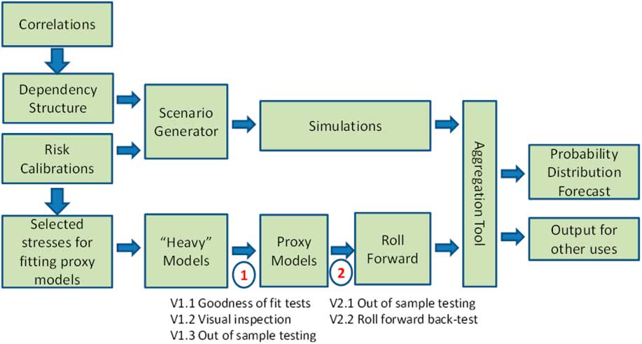
Figure 18 Internal model components and validation points
Hence, the scope of this section is validating the components at points labelled (1) and (2) in Figure 18 (Table 16).
Table 16 Proxy Model Validation Points

4.6.3 In-sample testing (goodness of fit and visual inspection)
An element of validation should occur during the fitting process. After regression is used to fit the curves, firms should output a number of fitting statistics to inform how well they have been able to fit the observed points. This is likely to include:
-
∙ R 2 or R – a measure of overall correlation and explanatory power.
-
∙ Mean squared error (MSE), or SSE. Both measures of the absolute fitting error.
-
∙ Maximum (absolute) error.
-
∙ Number of points outside a desired range – either an absolute or percentage amount.
These kinds of statistics are commonly used as part of OOS testing, so are discussed in the next section. Firms are also likely to use visual inspection to assess the fit. Statistical testing of in-sample points has limits on its credibility, because it does not cover the risk of un-modelled points being incorrect. If the user has sufficient expertise, graphical inspection can help to identify areas where the fit is inappropriate. For example, the fitted curve may show over-fitting or turning points outside the fitting range that we may not expect.
This is illustrated in Figures 19 and 20, which shows the hypothetical equity risk proxy function from Figure 16 in section 4.2 fitted using a polynomial of degree 5 (Figure 16 showed a polynomial of degree 2, and the same fitting points have been used to fit the degree 5 polynomial). Figure 19 illustrates how over-fitting to fluctuations between fitting points can result in an unintuitive proxy function within the fitting range. While Figure 20 shows the proxy function over a slightly wider range, which shows the effect of the unexpected turning point introduced is to suggest a £4bn loss in the event of +140% equity returns.
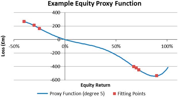
Figure 19 Degree 5 polynomial equity proxy function illustrating over-fitting
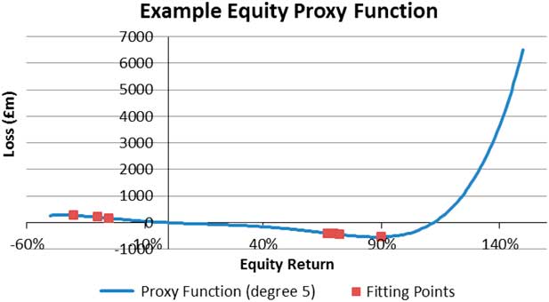
Figure 20 Degree 5 polynomial equity proxy function illustrating turning points beyond fitting range
4.6.4 OOS testing
OOS testing is an example of an effective statistical process for validating the proxy model. Scenarios that are not used in fitting are evaluated using the heavy model and compared with the results using the proxy model. The same sorts of fitting statistics can be used as for in-sample testing. Graphical inspection of the fitted curves themselves may have limited use in OOS testing because we are generally concerned with looking at multivariate points.
OOS testing tests for the impact of the following potential errors in proxy models (Table 17).
Table 17 Types of Errors Encountered in Proxy Modelling

Proxy models inherently contain an element of approximation and, as discussed in Hursey et al. (Reference Hursey and Scott2014), errors in individual points do not themselves invalidate the model. What is more important is that there is no bias in the fitted functions, so that the model does not systematically under- or overstate the result; or fail to adequately rank risks. Proxy model errors when assessing the Probability Distribution Forecast can be put into two categories:
-
(1) Proxy functions are biased so that the magnitude of losses is incorrect, though the ranking may be broadly correct, for example, where extreme losses are overstated by loss functions but would still be extremes in the ranking if the loss functions were accurate;
-
(2) Proxy functions are biased so that both magnitude and ranking of losses is wrong. This can arise, for example, due to turning points calculating profits when there should be losses (and vice versa) or where interactions are inaccurately modelled such that some combinations of risk have effects which are completely unexpected, for example, where a fit is accurate for scenarios when two risks both increase, but the wrong sign when the risks move in different directions.
In the former case, the model’s ability to rank risk may be appropriate, but the financial outcomes are not. For example, Economic Capital may be over or understated. Validation statistics would show that the proxy model is systematically over or understating the heavy model evenly across the full Probability Distribution Forecast.
In the latter case, the validation statistics would show errors that are not similar across the full Probability Distribution Forecast.
The reminder of this section focusses on the choices that need to be made when conducting OOS testing, and how to communicate the results.
4.6.5 Choosing scenarios for OOS testing
4.6.5.1 Number of scenarios
The Working Party is not aware of any specific approach to deriving a theoretically robust number of scenarios to test, for example, a formula based on statistical significance. Such approaches rely on the underlying assumption of randomness of errors which does not necessarily apply when replicating an underlying model.
Clearly the more scenarios tested the greater the confidence in the view formed from the tests on whether or not the proxy model is a good representation of the underlying heavy models.
The following principles are relevant in determining a suitable sample size ( Table 18).
Table 18 Principles to Determine the Number of Out-of-Sample Scenarios

A 2014 survey (Deloitte MCS Limited, 2014) of nine UK firms showed that the number of scenarios tested at the calibration date ranged from 20 to 1,000 (median 50), with a smaller number of scenarios also tested at the validation date. Clearly, time and cost are key limitations and constrain what companies can do; technological advances may mitigate this.
We expect the industry will refine its view of the suitable volume of tests as firms gain further insights from the testing they perform. They may then also become more focussed in their testing. Until then the approach is likely to be driven by the maximum achievable number within reasonable constraints.
4.6.5.2 Allocation of the scenario budget
It is important to test the full range of the scenarios across the Probability Distribution Forecast because different regions are relevant for different uses of proxy models.
Because we are looking to test the Probability Distribution Forecast, which is a representation of the full distribution of all the risk factors to which a company is exposed, the emphasis should be on testing multivariate points covering all risks. This ensures that the points tested can be mapped to the overall percentiles (and in fact are likely to be derived from percentile outputs of the model). This is useful for ensuring that interactions between risks are captured.
Scenarios that consist of a subset of risks can be appropriate when we are looking at a specific section of the model (e.g. asset, product or entity), which may be the case if the model is being used for a specific purpose, or if there are investigations that need to be performed after issues have been identified with the multivariate scenarios.
Notwithstanding the need to assess the full Probability Distribution Forecast, firms may choose to model a higher concentration of points at different percentiles, as ultimately different points will be more relevant for different uses of the model. The following table sets out an example target allocation of the number of scenarios across percentiles for a reporting entity. For this purpose, the percentile range has been split into six sections broadly aligned to usage. The scenarios are allocated across these percentiles in each fund to test various uses (Table 19).
Table 19 Allocation of Out-of-Sample Scenarios

SCR/Economic Capital: The simulations around the 99.5th percentile are most relevant for calculating the aggregate 1-in-200 capital requirement. The SCR or other Economic Capital measures are typically calculated as the 99.5th ranked loss across a large number of simulations.
The SCR can be under or overstated if there is a systemic error across many scenarios. For example, the SCR will be understated if proxy function fitting errors cause losses on simulations ranked at percentiles lower than the 99.5th to be understated, where, if the fitting error was not present, those simulations would result in a loss greater than the SCR. The understatement in SCR will depend on the extent of understatement in each simulation and how close they are to the 99.5th ranked loss.
As the 99.5th percentile will not be known until the proxy model has been run, a firm will choose OOS scenarios using results from previous calibration of the model (which they may roll-forward to the current reporting date, as we will touch on in section 4.6.10).
To test ranking errors, simulations near the 99.5th percentile are important. The further away from this region the greater the error needs to be to influence the ranking, although large errors are still possible where turning points exist. Systemic errors can be detected from anywhere in the range.
Diversified risks (or allocated capital): Diversified losses by risk are referenced for a number of purposes, including materiality definitions, risk appetite and prioritisation for risk management. A typical method of calculation is to take the average level of risk across simulations ranked from say 1,000 simulations around the 99.5th percentile, possibly weighted to give more weight to simulations near the 99.5th. The range of (in this example) 1,000 simulations is often known as “critical region” or “smoothing window”.
The accuracy of scenarios across the smoothing window is important to the accuracy of the diversified losses, and a firm may therefore wish to ensure these are covered by its OOS testing.
Short-term solvency estimation: Proxy models are commonly used to estimate changes in the economic balance sheet position between full calibrations. Typically, these are smaller movements that are actually experienced, both positive and negative. Testing scenarios at other percentiles will provide useful information on the accuracy of proxy functions in scenarios that might be encountered for this purpose. There is no specific percentile that needs to be focussed on for this purpose, but a range of levels close to the median (e.g. between the 30th and 70th percentiles) should be tested.
Risk appetite limits: Some insurers use proxy models to periodically set the level of capital needed to cover SCR after a 1-in-X level event, typically a 1-in-5 (80th percentile), a 1-in-10 (90th percentile) and a 1-in-25 (96th percentile). Proxy models are used to estimate the impact of these events on Own Funds and on SCR by assessing a 1-in-200 loss after the 1-in-X event.
Therefore, the adverse range below the 99.5th smoothing window needs to be tested for the Own Funds impact. Scenarios above 99.5th will therefore be relevant to validate the capability of loss functions to calculate the SCR after a 1-in-X event.
Stress and scenario testing (SST): Firms can use proxy models to assess Own Funds and SCR impacts after a defined scenario – which may be a 1-in-X scenario generated or a real-life defined scenario such as a pandemic. The testing in regions described for risk appetite setting is also suitable for validating the use of a proxy model for SST.
4.6.5.3 Scenario selection method
Scenarios may be either selected to target specific combinations of risks or selected non-systematically, such as at random or from pre-defined percentiles of the aggregate distribution.
Examples of the specific selection approach include:
-
∙ Targeting specific key interactions in each fund.
-
∙ Targeting outliers, for example, large credit scenarios.
-
∙ Targeting known limitations/poor fits.
Systematic approaches have the following challenges/disadvantages:
-
∙ They introduce potential bias towards poor fits.
-
∙ There are many potential permutations of interactions and probability levels that theoretically might be relevant. For example, a test pack for an annuity fund could include various pairs or triples of interest rate level, interest rate slope, longevity and credit and then with each at different probability levels and directions. It is difficult to judge the most appropriate and efficient subset of the permutations for testing. Over time, repeating the validation on new sets of simulations should build up a body of evidence that will test a wide range of these permutations and therefore continue to enhance understanding and help further refine the loss functions.
-
∙ It is manually intensive to find simulations that exhibit the required features and it can be the case that very few simulations in the relevant region exhibit material occurrence of particular interactions targeted.
4.6.6 Acceptance criteria
In order to assess whether the proxy model is fit for purpose, there is a need to define what is an acceptable deviation from the heavy model results, that is, what dictates a validation “pass” or “fail”.
The selection of tolerances for this purpose is one of the most important steps in the fitting and validation of proxy models. Tolerances determine the level of effort required in terms of the number of valuation model runs and the required complexity of the proxy model. In general, the lower the tolerances the higher will be the number of scenarios required in fitting and validation.
Setting arbitrarily tight tolerances may be spurious accuracy that will drive significant additional cost without altering management decisions. Setting tolerances which are too loose may lead to inappropriate decisions.
4.6.6.1 Setting tolerances
One way of setting tolerances is a top-down approach starting with management’s acceptability for the level of inaccuracy for each use of the proxy model and cascade down to individual scenario level as follows:
-
(1) Agree the level of accuracy required so that the model ranks risk sufficiently accurately and help senior management to make business decisions. What level of error in the key output, for example, SCR, risk appetite levels would drive management to alter a decision.
This is aligned to the definition of materiality in article 222 of the Solvency II Delegated Regulations (2015).
“For the purposes of this Chapter, a change or error in the outputs of the internal model, including the Solvency Capital Requirement, or in the data used in the internal model shall be considered material where it could influence the decision-making or the judgement of the users of that information, including the supervisory authorities”.
-
(2) At the same time the tolerances should be set in such a manner that the effort required in achieving them is (a) proportionate, (b) not unduly onerous to implement, and (c) makes allowance for accumulation of errors. This may lead to a simple high-level percentage or absolute error.
-
(3) Based on this high level tolerance, define the tolerances at lower levels, for example, legal entity level or sub-fund level or at individual risk level.
Tolerances may differ in different regions of the Probability Distribution Forecast reflecting that the SCR/diversified risk levels are likely to drive more risk management actions than say errors in very extreme scenarios. However, this may overcomplicate the validation operationally and require more scenarios in each region to get a representative view.
4.6.7 Validation measures
Firms should consider a range of statistics when analysing their OOS results. This should be a combination of descriptive and analytical statistics, and can include:
Measures of fit for individual samples:
-
∙ Monetary error (versus heavy model) in relevant currency.
-
∙ Percentage error, for example, as percentage of true heavy model result.
Descriptive measures for the full sample set:
-
∙ Number of samples outside a specified range (defined as monetary value).
-
∙ Number of samples outside a specified range (defined as percentage).
-
∙ Number of under- or overstatements.
-
∙ MSE.
-
∙ Mean absolute error.
Analytical statistics:
-
∙ R 2 (coefficient of determination)Footnote 3 . Measures how much of the variation in the heavy model result is explained by the proxy model. A value close to 1 (say ˃0.99) is expected if the proxy model is a good predictor of the heavy model.
-
∙ R (Pearson product–moment correlation coefficient). This measures the linear dependence between values from the fitted function and the in-sample modelled values.Footnote 4
-
∙ Coefficient of skewness: This is a measure of the extent to which the errors are biased in either direction (over-/understatement of heavy model result). This can tell us at an overall level whether the proxy model tends to under- or overstate results.
For the majority of these statistics, we can view the results across the whole loss distribution, or for specific regions of interest. This is particularly pertinent when looking at the skew of the errors. The skewness statistics could be low for the distribution as whole, but may contain clustering of bias at certain points of the curve. This is where graphical inspection of the OOS points can be instructive, since patterns in the residuals can be plotted and assessed accordingly.
4.6.8 How should the errors be investigated?
Individual errors can flag types of risk combination that are particularly inaccurate, for example, due to a missing or inaccurately modelled interaction (e.g. this can be identified by plotting OOS error against risk factor values and looking for systematic features). It may be that such combinations are rare and therefore the fail is not particularly important or it may be that the error occurs in many simulations and therefore causes errors across the Probability Distribution Forecast.
The cause of the failing individual scenario should be understood (or at least the unique features of the scenario compared with the passing scenario should be identified) and the simulation set examined to establish how frequent that type of scenario is to determine if further remedial action is justified due to pointing to a more systemic issue.
As well as looking at individual errors, a firm should examine the errors across all scenarios collectively. While individual errors may be within tolerances, this analysis could highlight systematic misstatements such as bias at a particular part of the loss distribution. For example, a firm could test for whether the number of over- or under-statements is statistically significant under the null hypothesis that the number of each follows a binomial distribution with an equal probability of over- or under-statement (parameter p=0.5).
4.6.9 Communicating validation results
The validation results can be communicated in the form of a plot showing the probability level of the chosen scenarios and how they relate to uses of the Probability Distribution Forecast.
An example of an effective plot for showing validation results is Figure 21. This is a scatter plot of proxy model result (y-axis) against the heavy model result (x-axis) for a set of OOS scenarios. If the proxy model were to produce exactly the same results as the heavy model, all points would fall on the dashed line. The plot allows us to compare the proxy model result to the heavy model result at different points of the loss distribution, and can be used to identify features visually such as:
-
∙ size and spread of residuals – seen from the vertical distance of a scenario, or cluster of scenarios, from the dashed line;
-
∙ large individual errors – as shown for two scenarios where the proxy model produces a result which is far from that of the heavy model;
-
∙ systematic under or overstatements – for example, in the region of the 50th–80th percentiles above where OOS results are clustered above the dashed line, indicating possible systematic overstatement of losses in that region.
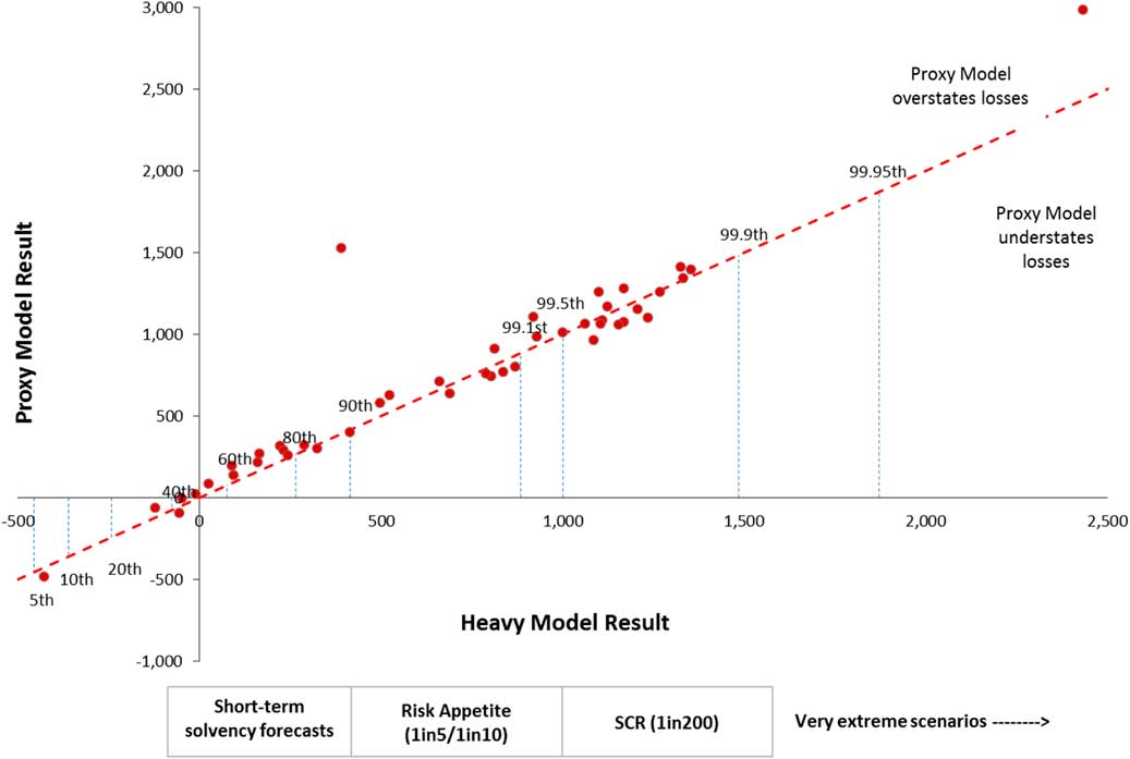
Figure 21 Plot of proxy model losses against heavy model losses; SCR, solvency capital requirement
This plot can be used to communicate the suitability of the proxy models to the users of the model for each of the use types. The plot helps to highlight the percentiles and situations where the fit of the model is good and where it is poor/uncertain and the impact that can have on the key output for each model use. This will help management understand the limitations of the model and therefore assist the user to adjust use accordingly rather than over rely on it where it is less accurate.
A box–whisker plot, or a histogram of errors, can also provide an informative summary of OOS results.
The graphical plots can also assist in understanding the distribution of residuals across the range of percentiles. This can bring out any issues that are present in certain areas of the curve, but which are lost when statistics are calculated for the full sample set (such as, e.g. the large individual errors shown on Figure 21).
4.6.10 Roll-Forward
4.6.10.1 Drivers for using roll-forward
Roll-forward is a fairly common practice used in producing the Probability Distribution Forecast at the valuation date in order to meet tight reporting timescales. It involves fitting the proxy model at an earlier date (e.g. end of Quarter 3) and then adjusting the fitted model to the valuation date (end of Quarter 4) using approximate scaling factors. This is an important consideration for reporting economic capital for multiple reasons including:
-
∙ To inform timely management interventions to manage risks.
-
∙ To meet expectations of the market for external reporting in the case of shareholder owned companies.
-
∙ To meet regulatory reporting requirements.
The required timescales may leave insufficient time to fully calibrate and validate proxy models using asset and liability data at the reporting valuation date. Instead actuaries have developed techniques that are designed to provide sufficiently accurate results with less dependency on data at the valuation date by “rolling forward” from previously calibrated models.
Typically, these techniques involve:
-
∙ Calibration off-cycle in advance of the reporting period.
-
∙ Roll-forward methodology to approximate the impact as at the valuation date of experience in the period since the calibration.
-
∙ A trigger framework to flag the need to intervene should the approximations exceed tolerance for inaccuracy.
4.6.10.2 Roll-forward methods
Roll-forward methods include:
-
∙ Scaling some proxy functions according to a readily available “carrier” for the movement in risk, for example, policy counts, sum assured or annuity payments in force – essentially some approximate measure that does not involve a heavy model calculation (such as best-estimate liability). Such risk carriers may capture changes in volume or changes in sensitivity or both. This may involve scaling proxy functions using a reduced volume of heavy model runs at the valuation date.
-
∙ Partial recalibration, for example, to focus recalibration on lines of business that are most sensitive to risk factors, or recalibrate the most material risk factors only, leaving proxy functions for other risks unchanged.
The choice of roll-forward method for a particular risk depends on:
-
∙ The materiality of the risk.
-
∙ The stability of the exposure to the risk.
-
∙ What circumstances might cause the magnitude of the risk to change materially.
4.6.10.3 Validation considerations
Roll-forward will potentially introduce additional approximation error over the proxy model calibration errors discussed earlier. A firm should ensure that both the calibration and roll-forward are operating appropriately; and that the aggregate error is within the firm’s tolerances, described in section 4.6.6.1.
Firms could perform validation at:
-
∙ The calibration date and then perform an analysis of the movement over the roll-forward period. The latter would be considered “light” validation of the roll-forward, and could for example, include stepping through each change to the proxy functions and risk factors to understand the cause of change and assess its reasonableness. Because this validation is light, it is best suited to more benign environments, for example, where the exposure to risk is stable, there is a fairly stable mix of business, when investment markets have been stable, or if the roll-forward period has been short.
-
∙ The valuation date only. This will most directly validate the model at the point at which it is being used. However, depending on the timescales for reporting, this may be a significant challenge.
-
∙ Both the calibration date and valuation date. For example, firms could test intensively at the calibration date, and then perform a smaller amount of testing at the valuation date before reporting deadlines.
The relative merits of each approach are discussed below.
OOS testing at the date of calibration:
-
∙ A cleaner controlled validation as we do not have roll-forward approximation affecting the validation results.
-
∙ The validation can easily be completed on-cycle before results are reported.
-
∙ However, this only the tests the proxy model at the point of calibration. Roll-forward would need to be validated separately; at a minimum an analysis of movement over the period can be used to back up the results from the proxy model. However, in non-benign conditions, or where the roll-forward period is long, this analysis may be difficult to reconcile. Therefore, it may be necessary to produce some amount of OOS testing at the valuation date.
OOS testing at the date of reporting:
-
∙ This most directly validates the specific result reported, and it tests both proxy model calibration and roll-forward combined.
-
∙ It will be difficult to complete on-cycle as we cannot start until roll-forward results are available, and reporting deadlines may be short.
-
∙ It can be harder to determine root cause of failing scenarios without significant additional work to isolate roll-forward errors from proxy model errors.
Current practice varies across the industry. Most firms perform a substantial amount of testing at the calibration date. Many firms also perform a smaller amount of testing at the valuation date (Deloitte MCS Limited, 2014).
An alternative mitigant, for those firms who do not wish to conduct further significant testing at the valuation date, would be to investigate and set trigger points. These trigger points would be designed to set limits at which the firm would start to doubt calibration of the proxy functions. These trigger points could relate to a number of things, for example:
-
∙ Large market changes – market movements that are severe enough to cast some doubt as to the appropriateness of the proxy functions, particularly for assessing a 1 in 200 level of confidence after the market movement, which may be very deep in the tails of the original calibrated proxy function.
-
∙ Business experience – large levels of lapses or new business, in particular if these are concentrated on certain products such that scaling of proxy functions may not represent the true movement in exposure to risk.
-
∙ Other business activities, such as changes to investment policy, new or altered reinsurance treaties or hedging strategies. The existing proxy functions may not be easily adaptable for these types of events.
There will usually be a degree of subjectivity involved in setting any trigger points, so the firm should be realistic in answering the fundamental question of what would invalidate the calibrated proxy model.
4.7 Proxy Model Fitting: Limitations and Acceptance
When considering limitations in the fit of a proxy model, we should always have in mind the use of the model. A fitting issue may invalidate a proxy model’s use for one purpose but it may still be acceptable to use it for other calculations.
The goodness of fit of the proxy models may be limited in a number of different ways.
-
∙ Particular products/risks do not fit well. This may be acceptable if they are not material. Poor fit for individual products may be satisfactory at entity level for an SCR calculation, but the model should be rejected for product level reporting. Also firms should be wary of improving fit in some areas but not others, as this can distort the quality of fit higher up the hierarchy.
-
∙ Poor fit at legal entity level could lead to misstated financial results, and must be rectified. It is also likely to imply poor fit at other levels of the aggregation, for example, product level.
-
∙ The quality of fit may differ at different regions of the Probability Distribution Forecast. If the fit at extreme percentiles is poor, it may still be possible to use the model for calculations that involve more central percentiles, such as estimating balance sheet movements from short-term changes in risk factors.
-
∙ The model may contain over-fitting to particular aspects. For example, it may include lots of cross-terms and be calibrated using a high volume of multi-dimensional points, however, this may compromise fit for univariate risks at important points. This could cause problems when monitoring individual risk exposures.
The above points need to be taken into account in determining what constitutes model failure. Indeed, there could be many forms of failure, and so it is important to clearly link the nature of the failure to the use of the model. As a result, a proxy model may be accepted for certain uses but not others.
Section 4.6.6 described the need for a firm to set tolerances for use in validation of their proxy model. If these tolerances are not met, the firm will want to try and remedy this, for example, increasing the number of fitting points or manual intervention in any mathematical fitting exercise. However, this will take time to do and with accelerated reporting cycles it is highly likely that this will not be possible within the timescales of results submission. One mitigant of this would be to conduct curve fitting exercises “off-cycle”, as described in the roll-forward section, so that such issues can be addressed in advance of the reporting cycle.
It may be the case that the model fails for a particular use, for example, the fit may be inadequate around the centre of this distribution, but well fit in the tails – perhaps because fitting has concentrated on that area. In such a case, the reasonable decision would be to accept the model for use in tail risk calculations, but not more moderate stresses, such as one may apply when performing roll-forward calculations. Subsequently, a firm may then consider recalibrating off-cycle to achieve a better fit in the middle of the distribution.
Note that the reverse would likely present more problems, that is, inadequate tail calculations are likely to cause a problem in calculating an SCR in required timeframes. In such a case, there are a range of options that could be considered to deliver a result in the time required and these are discussed in the next section.
4.7.1 Mitigating a poor proxy model fit
Above we described ways in which the fit of a proxy function may not meet a firm’s tolerances. We noted that it may not be possible to re-perform the fitting process within the reporting cycle. As such, this section outlines some ways in which a firm may mitigate a poor fit.
4.7.1.1 Use a previous calibration
It may be better to use a previous accepted calibration with roll-forward from that calibration date. However, one should be cautious with this as there may have been fundamental changes that have caused the failure for the latest calibration. This would imply that the previous calibration may not be a suitable reflection of the risk exposures. It may alternatively imply that there has been a mistake or otherwise poor choice in the latest fitting exercise, and it would be preferable to revert to the previous calibration. Note that it should be possible to only re-use the failing proxy functions, rather than the full set. Using historical calibrations moves us further from the “live” position, so adequate OOS testing should be performed on the “rolled forward” loss functions (to the extent this is possible in the time provided).
4.7.1.2 Adjust proxy model results
One option is to apply an end-piece adjustment to the results of the proxy model to reflect the invalid fit, but this should be viewed only as a temporary solution and a firm should seek to rectify the underlying cause of poor fit in its subsequent development cycle.
For example, a firm could adjust the previous calibration and results from that model, as well as use any other information available (such as analysis of movement or roll-forward information), to form a view on what the firm expects the result to be. This may be supplemented by prudent adjustments.
4.7.1.3 Use OOS results to improve fit
Where an issue with proxy model fit is identified during in-cycle reporting, it would be desirable to use OOS results to improve the fit where it is possible to do so, as an alternative to running additional (or alternative) fitting scenarios. However, techniques for doing so, of which the Working Party is aware, are as follows:
-
∙ Add the OOS scenarios to the fitting set and recalibrate proxy functions. However, the firm would need further OOS points for validation, as using these additional points could potentially create new errors in other parts of the proxy model.
-
∙ Include OOS errors as an empirical proxy function (as described in section 4.5.3.2) within the proxy model. Evaluating this proxy function would estimate the error in each simulation which would be added to the results of the other fitted proxy functions. This has the advantage of not requiring the firm to recalibrate its proxy functions, and hence not distorting areas of the curve which may be well fit. However, the method requires the model to interpolate between the OOS points in order to estimate the loss for all other points. Hence, it may be a more appropriate method in areas where we have a higher concentration of OOS points, for example, around the 99.5th percentile.
-
∙ Use OOS results to calibrate adjustments (e.g. a shift or scaling) to proxy functions, and apply these adjustments to the proxy functions used in the simulation. For example, if a linear relationship between OOS errors and heavy model losses exists, a firm could fit a linear function using regression techniques. This function can then be applied as an adjustment to proxy function results in each simulation which reduces the effect of the error on average.
-
∙ The mean error on OOS scenarios in a particular region of the Probability Distribution Forecast could be added to estimates of quantiles in that region. For example, the mean error in the OOS scenarios in the region of the SCR (i.e. scenarios within a particular percentile interval around the 99.5th percentile, for example, 99.4th–99.6th percentiles) could be added to the estimate of the SCR which was produced by a simulation approach, as an adjustment for bias in proxy functions at that point.
4.7.1.4 True-up to biting scenario
For the purposes of calculating Economic or SCRs using a VaR approach, fitting errors could be addressed through a biting scenario run through the heavy models for part or all of the relevant business. In this case, a firm would use their proxy model to determine the combination of risks which occur at the biting scenario, and evaluate that scenario in their heavy models. They could then apply an adjustment to the proxy model result equal to the difference between the results. In order to do this, a firm must be able to justify using the biting scenario derived by its proxy model, particularly if it has not passed validation triggers. However, we note that this can be performed in addition to some of the other adjustments above to refine the fit.
The unsmoothed biting scenario is the single scenario at the percentile of interest in the loss distribution. This may contain an extreme adverse stress in one particular risk, which is not representative of the overall combination of risks which leads to the capital requirements. This scenario may happen to have a poor fit, which is not representative of the quality of fit in the region of the percentile, and so any adjustment for fitting errors which is derived by considering the error at this single scenario may not be appropriate.
It is therefore common to calculate a smoothed biting scenario, for example, by averaging risk factors across a number of simulations around the percentile of interest. This scenario is more representative of the risks which combine to create the capital requirement; however, some risks (e.g. hedged risks where losses occur under both up and down risk factor movements) may average out to zero. This may mean that the smoothed scenario does not contain a combination of risks which would result in the capital requirement.
4.8 Addressing the Communication Challenges
Section 4.3 outlined some key communication challenges with respect to using proxy models. The above sections have described how proxy models can be designed, fitted and validated. Building from that, Table 20 discusses how these communication challenges can be met.
Table 20 Communication Challenges and Responses

5 Conclusions
5.1. One of the most fundamental choices to be made in the construction of any economic capital model is how to aggregate together the capital requirements for the individual risk factors and take account of the effects of diversification. The correlation matrix approach to aggregation commonly adopted by UK life insurers under the ICAS Framework is unlikely to be adequate for some life insurers to meet the Solvency II requirements for use of a “full Probability Distribution Forecast”. This has led some life insurers to use more sophisticated approaches to the aggregation of capital requirements in their Internal Model used to calculate the Solvency II SCR such as the “copula + proxy model” approach described in this paper.
The aim of this paper was to provide UK life insurance actuaries with some examples of techniques which could be used to test and justify recommendations relating to the aggregation approach. The paper includes some practical examples of how those techniques may be communicated effectively to stakeholders, but ultimately actuaries should choose techniques which are most appropriate to circumstances of the individual undertaking and the stakeholders involved. For some stakeholders, graphical techniques provide a compact way of illustrating concepts and discussing alternative assumptions. Such techniques may prove more effective in engaging stakeholders whilst avoiding unnecessary technical detail.
5.2. For most UK life insurers, the limited volume of relevant data and the practicalities of modelling, parameterising and using a copula, means that the choice of the copula model has so far been limited in practice to the Gaussian or Student’s t model. Each of these has its limitations for which the undertaking will have to allow when parameterising and using the model. For an individual undertaking, the specific choice comes down to prior beliefs and preference for modelling tail dependence explicitly or adjusting for it by making allowances within the parameterisation. In section 3.5 we explained how the parameterisation of a Gaussian or Student’s t copula could be built up using a “bottom-up” approach. We discussed several different techniques by which data could be used to inform the allowance made for tail dependence and the choices illustrated using graphical techniques. All of these techniques have strengths and limitations. Ultimately it is a question of judgment, including the choice of copula, as to which method is most appropriate.
Consideration must also be given to whether the resulting parameters are collectively reasonable and appropriate for the purposes for which they are used. Section 3.15 provided several examples of “top-down” validation tools such as peer review through expert judgement panels, sensitivity testing, scenario analysis and industry benchmarking.
5.3. We briefly discussed the use of goodness of fit tests or model filters to validate the choice of copula model in Section 3.16. Such tests may seem appropriate to demonstrate compliance with the statistical quality standards of Solvency II. However, the lack of relevant data means that, in practice, they are likely only to be useful for sets of homogeneous risks where there is a relatively rich set of data (e.g. equity returns in different geographies).
5.4. Proxy model designs can be influenced by the hierarchical structure or granularity of the model, constraints to diversification, tax impacts and associated risk factors. Fitting the proxy model includes defining the objectives, selecting the form of the proxy function and choosing the fitting method either via regression or interpolation. To validate a proxy model the actuary defines the validation scope and performs both in-sample and OOS testing. Communication of the suitability of the results can be done graphically by comparing the proxy model to the heavy model and communication challenges and how they can be addressed were presented.
5.5. Proxy modelling techniques, including copula-generated scenarios are not new, however, they have seen a recent resurgence in their use in insurance, having been used previously in the banking industry as well as other non-financial applications. Advances in computing power also made it more feasible. The method is relatively simple to develop and a number of providers market standard or tailored products to insurers. Of course, as we have seen, simulation techniques still present limitations, however, they address some of the key limitations of the correlation matrix approach. Crucially they can produce a continuous aggregate loss distribution of losses and they can point to a combination of risks that result in a certain amount of loss, relatively easily (sometimes referred to as “what-if” scenarios). Finally, they should also aid in meeting “use-test” requirements of Solvency II.
Simulation techniques also make more transparent the assumptions made implicitly in a correlation matrix approach and provide the user with greater flexibility to depart from them. Of course, simulation techniques in this area are relatively new in the industry, so probably no standard market practice has been established in a number of areas, but as its use continues to grow the costs of the copula+proxy model approach may fall over time.
Acknowledgements
The Working Party is grateful to Andrew D. Smith for helpful discussions and permission to reproduce the chart from Shaw et al. (Reference Shaw, Smith and Spivak2010) and material from his forthcoming paper “Arachnitude and higher order dependence” in section 3.10 (Smith, 2014). The Working Party is also grateful to Professor Alexander J. McNeil and Professor Marius Hofert for helpful discussions; to Stephen Makin, with whom some of the material of section 3.8 is joint work; to Frazer Dawson and Vincent He for permission to reproduce material on “correlation hardening” in section 3.9 and to Rob Harris for helpful comments provided throughout the drafting of this paper. The Working Party is also grateful to Scott McNeill, Peter Murphy, Tim Wilkins and Fraser Willis for their useful comments on draft versions of this paper. Finally, the Working Party would like to express its thanks to two anonymous peer reviewers for their helpful comments. The majority of the analysis in section 3 was performed using the R statistical package (R Core Team, 2013) and in particular using the R packages “copula” (Hofert et al., Reference Hofert, Kojadinovic, Maechler and Yan2015) and “QRM” (Pfaff & McNeil, Reference Pfaff and McNeil2013).
Disclaimer
The views expressed in this publication are those of invited contributors and not necessarily those of the Institute and Faculty of Actuaries. The Institute and Faculty of Actuaries do not endorse any of the views stated, nor any claims or representations made in this publication and accept no responsibility or liability to any person for loss or damage suffered as a consequence of their placing reliance upon any view, claim or representation made in this publication. The information and expressions of opinion contained in this publication are not intended to be a comprehensive study, nor to provide actuarial advice or advice of any nature and should not be treated as a substitute for specific advice concerning individual situations. On no account may any part of this publication be reproduced without the written permission of the Institute and Faculty of Actuaries.
A.Appendix
A.1. Date used in illustrations
Table A1 shows the data set used in illustrations of statistical techniques.
Table A1 Assumptions and Time Periods Used for the Risk Factors in Our Data Set

All analysis has been based on monthly increase in each risk factor during the period 31 December 1996 to 31 December 2014 (i.e. 216 data points).
A.2. Definition: pseudo-observations
Given a set of N observations of a one-dimensional random variable {X
1, … , X
N
}, the set of pseudo-observations {Y
1, … ,Y
N
} is defined by setting ${\bf{Y}} _{{\bf{i}} } \, {\equals}\, {1 \over {{\bf{N}} {\plus}1}}$
rank(X
i
) for i=1, … , N.
${\bf{Y}} _{{\bf{i}} } \, {\equals}\, {1 \over {{\bf{N}} {\plus}1}}$
rank(X
i
) for i=1, … , N.
In other words, the pseudo-observations are the ranks of the random variables, scaled so that they take values in the interval (0, 1).
It is usual to divide by (N+1) rather than N to obtain values which lie strictly between 0 and 1. This avoids singularities when using pseudo-observations in certain applications (e.g. maximum likelihood estimation).
Where a random variable X takes vector values, the pseudo-observations are obtained by applying the transformation separately for each coordinate.
A.3. Theoretical basis for approach based on higher rank invariants
The approach of Shaw et al. (Reference Shaw, Smith and Spivak2010) is based on a Fourier expansion of the copula density function in terms of (shifted) Legendre polynomials. In two dimensions, this takes the form:
 $$c\left( {u,v} \right)\, {\equals}\, {\mathop \sum\nolimits_{i\, {\equals}\, 0}^\infty \mathop \sum\nolimits_{j\, {\equals}\, 0}^\infty r_{{i,j}} \tilde{P}_{i} (u)\tilde{P}_{j} (v)\,{\rm for}\,0\leq u, v \leq 1$$
where c(u, v) is the copula density and $\tilde{P}_{i} $
is the shifted Legendre polynomial defined on the interval [0, 1]. The latter is related to the standard Legendre polynomial P
i
defined on the interval [−1, 1] by the formula
$\tilde{P}_{i} $
is the shifted Legendre polynomial defined on the interval [0, 1]. The latter is related to the standard Legendre polynomial P
i
defined on the interval [−1, 1] by the formula $\tilde{P}_{i} (u)\, {\equals}\, P_{i} (2u{\minus}1)$
. (For a definition of the P
i
see appendix C of Hursey & Scott (Reference Hursey, Cocke, Hannibal, Jakhria, MacIntyre and Modisett2012), Smith & Sweeting (Reference Smith2011) or any standard textbook on approximation theory.) The
$\tilde{P}_{i} (u)\, {\equals}\, P_{i} (2u{\minus}1)$
. (For a definition of the P
i
see appendix C of Hursey & Scott (Reference Hursey, Cocke, Hannibal, Jakhria, MacIntyre and Modisett2012), Smith & Sweeting (Reference Smith2011) or any standard textbook on approximation theory.) The $\tilde{P}_{i} $
(u)
$\tilde{P}_{i} $
(u) $ \tilde{P}_{j} (v)$
form an orthogonal basis for the set of continuous functions on [0,1]2 with respect to the usual L
2 inner product. The Fourier coefficients r
i,j
are determined by the formula:
$ \tilde{P}_{j} (v)$
form an orthogonal basis for the set of continuous functions on [0,1]2 with respect to the usual L
2 inner product. The Fourier coefficients r
i,j
are determined by the formula:
 $$r_{{i,j}} \, {\equals}\, \left( {2i{\plus}1} \right)\left( {2j{\plus}1} \right) \mathop \int \nolimits_{\left[ {0,1} \right]^{2} } c\left( {u,v} \right)\tilde{P}_{i} \left( u \right)\tilde{P}_{j} \left( v \right)du\,dv\, {\equals}\, \left( {2i{\plus}1} \right)\left( {2j{\plus}1} \right){\Bbb E}\left[ {\tilde{P}_{i} \left( U \right)\tilde{P}_{j} \left( V \right)} \right] $$
It can be shown that r 0,0=1 and r i,0=r 0,j =0 for i, j>0 – the latter being a consequence of the copula having uniform marginals.
Thus $c\left( {u,v} \right)\, {\equals}\, 1{\plus} \mathop \sum\nolimits_{i\, {\equals}\, 1}^\infty \mathop \sum\nolimits_{j\, {\equals}\, 1}^\infty r_{{i,j}} \tilde{P}_{i} (u)\tilde{P}_{j} (v)$
, that is, the density function of the independence copula plus an additional term which introduces dependency. The formula generalises in the natural way to higher dimensions.
$c\left( {u,v} \right)\, {\equals}\, 1{\plus} \mathop \sum\nolimits_{i\, {\equals}\, 1}^\infty \mathop \sum\nolimits_{j\, {\equals}\, 1}^\infty r_{{i,j}} \tilde{P}_{i} (u)\tilde{P}_{j} (v)$
, that is, the density function of the independence copula plus an additional term which introduces dependency. The formula generalises in the natural way to higher dimensions.
The Fourier coefficients r i,j are uniquely determined by the copula and can be thought of as an array of characteristic values, analogous to the vector of moments of a one-dimensional distribution. Smith & Sweeting (Reference Smith2011) define the rank invariant called “arachnitude” as:
ρ((2F X (X)−1)2, (2F Y (Y)−1)2), where ρ is Pearson’s (linear) correlation.
The equivalent sample statistic is given by the formula
 $${\rm arachnitude}\, {\equals}\, {{45} \over {4N\left( {N^{2} {\minus}1} \right)\left( {N^{2} {\minus}4} \right)}}\left[ {\mathop \sum\limits_{k\, {\equals}\, 1}^N \left( {2R_{k} {\minus}N{\minus}1} \right)^{2} \left( {2S_{k} {\minus}N{\minus}1} \right)^{2} {\minus}{{N\left( {N^{2} {\minus}1} \right)^{2} } \over 9}} \right]$$
where the {R i } and {S j } are the ranks of the sample data {x i } and {y j }. Arachnitude takes values between −1 and 1 and is large when extreme high or low values of X tend to coincide with extreme high or low values of Y. It is therefore a measure of dependency along both diagonals rather than just along the 45° ray as in the case of tail dependence.
The Fourier coefficients of the copula and the rank statistics are related by the following formulae:
 $$ {{r_{{1,1}} } \over 3}\, {\equals}\, {\rm Spearman’s} \,{\rm rank}\,{\rm correlation}$$
 $${{r_{{2,2}} } \over 5}\, {\equals}\, {\rm arachnitude}$$
Further details are available in Smith (2014).
B. Appendix – Extracts from Solvency II Delegated Regulation 2015/35
Article 228
Probability distribution forecast
-
1. The probability distribution forecast underlying the internal model shall assign probabilities to changes in either the amount of basic own funds of the insurance or reinsurance undertaking or to other monetary amounts, such as profit and loss, provided that those monetary amounts can be used to determine the changes in basic own funds. The exhaustive set of mutually exclusive future events, referred to in Article 13(38) of Directive 2009/138/EC, shall contain a sufficient number of events to reflect the risk profile of the undertaking.
-
2. Insurance and reinsurance undertakings shall calculate the probability distribution forecast of a partial internal model at the highest level of aggregation of the components of the partial internal model. If a partial internal model consists of different components which are separately calculated and not aggregated within the partial internal model, the probability distribution forecast shall be calculated for each component.
Article 230
Information and assumptions used for the calculation of the probability distribution forecast
-
1. Information shall only be considered credible for the purposes of Article 121(2) of Directive 2009/138/EC where insurance and reinsurance undertakings provide evidence of the consistency and objectivity of that information, the reliability of the source of information and the transparency of the method by which that information is generated and processed.
-
2. Assumptions shall only be considered realistic for the purposes of Article 121(2) of Directive 2009/138/EC where they meet all of the following conditions:
-
(a) insurance and reinsurance undertakings are able to explain and justify each of the assumptions, taking into account the significance of the assumption, the uncertainty involved in the assumption and why the relevant alternative assumptions are not used;
-
(b) the circumstances under which the assumptions would be considered false can be clearly identified;
-
(c) insurance and reinsurance undertakings establish and maintain a written explanation of the methodology used to set those assumptions.
Article 234
Diversification effects
The system used for measuring diversification effects referred to in Article 121(5) of Directive 2009/138/EC shall only be considered adequate where all of the following conditions are met:
-
(a) the system used for measuring diversification effects identifies the key variables driving dependencies;
-
(b) the system used for measuring diversification effects takes into account all of the following:
-
i) any non-linear dependence and any lack of diversification under extreme scenarios;
-
ii) any restrictions of diversification which arise from the existence of a ring-fenced fund or matching adjustment portfolio;
-
iii) the characteristics of the risk measure used in the internal model;
-
-
the assumptions underlying the system used for measuring diversification effects are justified on an empirical basis.


 Open access