
8.1 Introduction
This chapter’s central thesis is that speech rhythm plays a critical role in the parsing and understanding of spoken language. Moreover, rhythm provides a sensory framework for low-frequency (3 Hz–25 Hz) acoustic modulations to interact with other modulatory signals such as visual speech cues. Such sensory modulation provides a potential gateway for accessing endogenous neural activity oscillating at comparable frequencies, hence facilitating cognitive access to linguistic information useful for interpretating inherently ambiguous acoustic signals. The rest of this chapter discusses a variety of experimental and theoretical evidence in support of this thesis.
8.2 A Brief History of Early Speech Modulation Research
The prosodic properties of spoken language have attracted a lot of attention in recent years (e.g., Loukina et al., Reference Loukina, Kochanski, Rosner, Shih and Keane2011; Ravignani and Norton, Reference Ravignani and Norton2017; Poeppel and Assaneo, Reference Poeppel and Assaneo2020). Some of this newfound interest is due to an increasing awareness that the linguistic (especially phonemic) models of yesteryear are not entirely in accord with how speech and often intense is processed in the real world, where background noise and reverberation are commonplace and often intense (Assmann and Summerfield, Reference Assmann, Summerfield, Greenberg, Ainsworth, Fay and Popper2004).
For many years, speech models focused on the signal’s spectral structure as the basis for decoding spoken language (e.g., Jakobson et al., Reference Jakobson, Fant and Halle1952/Reference Jakobson, Fant and Halle1963; Fletcher, Reference Fletcher1953; Ladefoged, 1968/Reference Ladefoged1995; Allen, Reference Allen, Ramachandran and Mammone1995; Stevens, Reference Stevens1998). These frequency-based models assume that processing of the speech signal amounts to linking spectral patterns with phonemic elements, which in turn are used to recognize words and other (e.g., phrasal) linguistic elements. In this context, “spectral” refers to the frequency analysis performed by the auditory system, one that provides a tonotopically structured profile (with respect to auditory neural discharge patterns) as a function of time (i.e., a frequency versus time representation) that some region(s) of the brain (presumably, higher-level language areas) associate with specific phonetic properties, either articulatory-acoustic features (e.g., Chomsky and Halle, Reference Chomsky and Halle1968; Jakobson, Reference Jakobson1968), “landmarks” (Stevens, Reference Stevens1998), or individual “phonemes” (e.g., Ladefoged, 1968/Reference Ladefoged1995), in a cognitive (and neurological) effort to infer the words spoken (in their appropriate sequence). The detailed mechanism(s) by which this neural time–frequency activity is linked to linguistic elements isn’t described in detail, nor is it a means for connecting such linguistic entities to higher-level constructs such as syllables, words, or phrases (and other meaningful elements).
Although there were clues early on that nonphonemic elements might play an important role (e.g., Dudley, Reference Dudley1939, Reference Dudley1940; Kozhnekov and Chistovich, Reference Kozhnekov and Chistovich1965; Liberman et al., Reference Liberman, Cooper, Shankweiler and Studdert-Kennedy1967), the spectral-phonemic perspective formed the foundation of mainstream speech research until recently. This spectral focus played an especially prominent role in automatic speech recognition (ASR) technology in which lexical models were based on strings of phonemic elements (hereafter “phonemes” [Rabiner and Juang, Reference Rabiner, Juang, Benesty, Sondhi and Huang2008]). Considerable effort was put into developing “language models” and “pronunciation dictionaries” to compensate for sub-par recognition of the phonetic constituents of the words spoken. Such systems required advance knowledge of the likely words spoken (“language models”) to have a reasonable chance of accurately inferring them (e.g., Jelinek, Reference Jelinek1998).
8.2.1 The Modulation Spectrum: Origins and Motivation
The seeds for an alternative approach, based on slow modulations in the speech waveform, were planted in the 1970s when the first steps were taken towards dethroning the spectral-phonemic framework.
The original goal of Houtgast and Steekeken’s (Reference Houtgast and Steeneken1973, Reference Houtgast and Steeneken1985) research was a practical one. They wanted a metric to predict when speech would be intelligible in a variety of listening environments (e.g., concert auditoria, theaters, and classrooms). They found that the acoustic properties most predictive of intelligibility (i.e., the ability to accurately report the words spoken in the correct order) were not spectral (i.e., acoustic frequency) but rather ones based on extremely slow modulations in the speech signal. How slow? So slow that when expressed in units of frequency, they were well below the threshold of tonal pitch (ca. 30 Hz). In other words, the key acoustic features for intelligibility are orthogonal to the classic spectral elements that had long dominated phonetics and speech research.
To quantify these very low-frequency modulations, Houtgast and Steeneken developed a novel method for their computation and visualization called the modulation spectrum. By analogy with the frequency spectrum, they measured the amount of energy in a bank of modulation-frequency filters. Highly intelligible speech, presented in high signal-to-noise-ratio conditions, exhibited a peak in the modulation spectrum at ca. 4 Hz–5 Hz. However, there was considerable energy down to ca. 3 Hz and up to ca. 12 Hz. The 4 Hz–5 Hz peak implied there was something special about syllables, whose durational properties (125 ms–250 ms) correspond closely to that time frame (when expressed in frequency units). The modulation spectrum turned out to be an excellent predictor of intelligibility because of its sensitivity to acoustic interference from reverberation (the result of acoustic reflections off hard surfaces such as walls, floors, and ceilings) or background noise (e.g., multi-talker speech babble or street noise). In extremely noisy environments, where intelligibility is severely degraded, they found that the peak of the modulation spectrum is significantly attenuated or even flattened.
Despite Houtgast and Steeneken’s compelling data, the modulation spectrum’s specific connection to intelligibility was left unresolved.
8.2.2 Modulation’s Role in an Early Form of Speech Synthesis
Deeper insight emerged in the 1990s when several studies investigated how low-frequency modulations in the speech waveform impact intelligibility. But before discussing this research, it’s helpful to summarize the pioneering research of Homer Dudley, an engineer working at Bell Laboratories in the 1930s. Dudley wanted to improve the quality of speech transmitted over the telephone (his workplace was a subsidiary of AT&T). To do so, he developed two analog tools, the voder and the vocoder (the latter being a more sophisticated version of the former). These were analog filter banks designed to “quantize” speech into a more compact form than the original signal allowed. In two groundbreaking articles (Dudley Reference Dudley1939, Reference Dudley1940), Dudley made a key distinction between the “carrier” associated with spectral features distinguishing phonetic segments (aka “temporal fine structure” [Smith et al., Reference Smith, Delgutte and Oxenham2002]) and the “modulator” (whose time course roughly follows syllabic elements). The latter was the precursor to what is now called the “speech envelope,” but it is important to note that Dudley’s original terminology applied to an engineering application designed to simulate human speech, not to a perceptual or neurological property.
In Dudley’s view, both the carrier and the modulator were essential for speech to sound natural and intelligible. Because the bandwidth of the telephone was limited in those days, Dudley sought to determine how much of the signal’s bandwidth could be reduced (i.e., “compressed”) without serious impact on intelligibility or quality. Dudley noted that a relatively small number (ca. 10) of frequency channels was required for the speech to be intelligible (and sound natural). Through this simple demonstration, the importance of auditory frequency analysis was demonstrated using a primitive form of what later came to be known as speech synthesis (or “text to speech”).
8.2.3 The Importance of Low-Frequency Modulations in Speech Perception
The broader significance of Dudley’s demonstration and Houtgast and Steeneken’s intelligibility assessment tool emerged with new research in the 1990s. The next step came from a group headed by Reinier Plomp (see Plomp, Reference Plomp2003, for a review of his research). One of Plomp’s students, Rob Drullman (Drullman et al., Reference Drullman, Festen and Plomp1994), performed, as part of his PhD research, a set of perceptual experiments in which the low-frequency modulations in the acoustic speech signal were selectively low- or high-pass filtered (keeping other acoustic properties untouched), and the impact of such manipulations on intelligibility were assessed. “Smearing” (Drullman’s term) of syllabic elements, resulting from low-pass filtering of the modulations in the speech signal, seriously impaired intelligibility. Listeners found it challenging to parse the speech stream into distinct, identifiable words. Drullman’s results were roughly consistent with Houtgast and Steeneken’s earlier studies. Modulation frequencies below 16 Hz were found to be essential for highly intelligible speech, and modulations in the vicinity of 3 Hz–8 Hz were shown to be especially important (in line with the intuition that syllabic elements are indeed important).
In the US, Shannon et al. (Reference Shannon, Zeng, Kamath and Wygonski1995) at the House Ear Institute used an updated version of Dudley’s vocoder to demonstrate the importance of low-frequency modulations using a novel method. In place of voiced speech, a broadband white noise signal served as the input to the vocoder. This noise signal was modulated by the original voiced version of the speech signal. In other words, the original speech signal’s fine time structure was replaced by white noise (i.e., equal energy per Hz band). The modulatory properties of the original speech signal were varied, along with specific details based on the spectral bandwidth and number of frequency channels. A single-channel modulator comprising the full spectral bandwidth of the signal (analogous to the speech envelope) was not intelligible. Only when the noise signal was filtered into four, eight, or more frequency channels were the resulting signals intelligible, indicating that the modulatory properties of the speech signal needed to be manipulated in a specific way. Another way of stating their finding is that a diversity of slow modulation patterns, derived from a broad range of distinct frequency channels, is essential for producing artificial speech that is readily understood. This noise-excited vocoder provided a demonstration that the rhythmic properties of speech could not be satisfactorily represented by a modulatory envelope derived from a unitary source (i.e., the full-band speech signal or even an octave-band signal derived from just a single region of the spectrum).
This key insight, buttressed by Drullman’s studies, suggested that the “speech envelope” is inadequate to fully characterize the rhythmic properties of speech. Instead, speech is most faithfully represented by a series of distinct low-frequency modulation patterns emanating from different parts of the tonotopically organized auditory array. How these tonotopically distinct modulation patterns give rise to a unitary sense of rhythm is not well understood.
At this juncture in the modulation story, my colleagues and I began a series of studies (summarized in Greenberg, Reference Greenberg, Greenberg and Ainsworth2006, Reference Greenberg2022) to delve deeper into how these low-frequency modulation patterns impact intelligibility, as described later in the chapter. But before doing so, let’s examine some early research on speech synthesis before returning to our consideration of slow waveform modulations.
8.3 Modulations and Rhythm in Speech Technology
A group of researchers in Japan sought to create more natural-sounding speech than was possible using Dudley’s original vocoder or through a different method known as vocal-tract-based synthesis.
Beginning in the late 1980s, researchers at ATR (Advanced Telecommunications Research Institute in Japan) began to experiment with high-quality recordings of human talkers speaking a broad range of different words that provided a comprehensive repertoire of phonetic, syllabic, lexical, and phrasal contexts (i.e., read sentences and paragraphs). The recorded material sounded very natural, so the key step to deploy this recorded corpus to generate novel material was to define the appropriate acoustic “target” units and then choose a closely matched snippet of speech and connect it to another snippet with minimum distortion. Digital splicing algorithms were developed to figure out which snippet most closely approximated the desired target for each linguistic element being modeled. This method is called unit selection (Iwahashi et al., Reference Iwahashi, Kaiki and Sagisaka1992; Black and Campbell, Reference Black and Campbell1995), which soon became the foundation for most high-quality speech synthesis in which novel words and sentences could be generated from the limited amount (often just several hours) of pre-recorded material. The next challenge was to figure out how to splice the chosen snippets together to produce an output that minimized “glitches” and other distortions to optimize intelligibility. The approach came to be known as “concatenative synthesis” and quickly became the dominant form of speech synthesis. Only in recent years has concatenative synthesis been superseded by more sophisticated (and more natural-sounding) methods (summarized by Karagiannakos, Reference Karagiannakos2021).
Concatenative synthesis’s key insight is that prosodic properties, such as tempo and meter, matter greatly, both for naturalness and intelligibility. By using spoken material as the core of the synthesis engine, the ATR researchers (implicitly) recognized the importance of low-frequency modulation patterns for producing high-quality spoken material.
Efforts to incorporate modulation models in ASR began in the 1990s (Greenberg and Kingsbury, Reference Greenberg and Kingsbury1997; Kingsbury et al., Reference Kingsbury, Morgan and Greenberg1998; Kanedera et al., Reference Kanedera, Arai, Hermansky and Pavel1999). However, these early efforts didn’t produce a true breakthrough due to their failure to “translate” modulation patterns into meaningful linguistic elements (as well as their failure to incorporate modulation phase appropriately into sub-word and lexical representations). Later efforts, using more realistic modulation models, improved word recognition slightly (e.g., Hermansky, Reference Hermansky2010; Avila et al., Reference Avila, Kashirsagar and Tiwari2019), but optimal utilization of modulation patterns and rhythm would have to wait until the advent of “attention” and “transformers” (and other broad-context approaches) to ASR in the late 2010s and early 2020s (e.g., Vaswani et al., Reference Vaswani, Shazeer and Parmar2017).
8.4 Modulation as an Integrative Framework
The power of modulation models lies mostly in their ability to integrate sensory (and cognitive) information across a range of scenarios that would otherwise be challenging for purely spectral models. This limitation of the spectral-phoneme approach is of prime concern, as listeners rarely converse in pristine (i.e., little or no noise) environments. Honking autos, infants crying, barking dogs, cocktail-party babble, and so forth can pose a challenge for decoding speech. In many listening environments, speech’s acoustic signature changes into something quite distinct from the waveform emanating from the speaker’s vocal tract. And yet most listeners have little difficulty engaging in social discourse under such conditions (much of the time).
The basis of such resilience is unclear, but low-frequency modulation patterns are probably key. The importance of these slow fluctuations may have to do with two other sources of low-frequency modulation – one sensory, the other neural.
Visual speech cues (aka “speech reading”) can facilitate comprehension, especially in challenging environments (Grant and Walden, Reference Grant and Walden2000) and for the hearing-impaired (Grant et al., Reference Grant, Walden and Seitz1998). The opening and closing of the lips, the up and down motion of the jaw, the to-and-fro movement of the tongue, provide a coarse visual analog of certain features of the waveform’s modulation (see Chapter 2). Such visual cues are associated primarily with two linguistic features: “place of articulation” (Skipper et al., Reference Skipper, van Wassenhove, Nusbaum and Small2007), which serves to distinguish among certain consonants (e.g., [p] versus [t] versus [k]), and syllable dynamics germane to lexical and post-lexical parsing (Grant and Walden, Reference Grant and Walden1996). So important are visual cues that their presence can transform largely unintelligible signals into readily understandable speech in challenging listening conditions (e.g., background noise, multi-speech babble, extreme reverberation [Grant and Walden, Reference Grant and Walden2000]). Why is this sensory boost so important for modulation models?
It is likely because of the interaction of distinct but complimentary cues capable of providing the sort of linguistic specificity required to successfully decode the speech signal across a broad range of listening conditions. For example, place-of-articulation information is most closely associated with acoustic frequencies between 1,500 Hz and 3,500 Hz (Stevens, Reference Stevens1998), while syllable parsing is most facilitated by that region of the spectrum ca. 3 kHz (Grant and Walden, Reference Grant and Walden1996). It is the blending of classic phonetic cues with prosodic information that likely provides the foundation for speech intelligibility and comprehension.
8.5 The Speech Envelope as a Model of Auditory Modulation
The “speech envelope” is often used as a proxy for auditory neural activity in studies of linguistic rhythm (e.g., Aiken and Picton, Reference Aiken and Picton2008; Ding et al., Reference Ding, Patel and Chen2017; Oganian and Chang, Reference Oganian and Chang2019; Poeppel and Assaneo, Reference Poeppel and Assaneo2020). The envelope’s popularity stems from its ability to portray modulation in simple terms (e.g., Figure 8.1). It aids the visualization of neural activity that may be associated with such rhythmic qualities as speaking rate, metrical beat, and prosodic meter.
The speech envelope illustrated.
The “speech envelope” for a single sentence (shown in black). The temporal fine structure is portrayed in very light gray. Syllable boundaries are indicated by dotted vertical lines. The contour shows the “rate of change” in envelope energy, analogous to “delta features” used in certain ASR applications. Note how coarse the speech envelope is relative to the speech signal’s finer details. The envelope contour pertains to the broadband, unfiltered signal.

Figure 8.1 Long description
A line shows the envelope of the sound, tracing the peaks and valleys. Another line shows the positive rate of change of the sound's amplitude. The dotted lines mark the perceived boundaries between syllables. Other arrows point to the peaks of the envelope, indicating the highest amplitude points. Other arrows point to the peaks of the positive rate of change, indicating the steepest positive slope in the sound's amplitude. A text at the top of the graph reads, It had gone like clock work.
However, the term “speech envelope” is potentially misleading, as there is no physiological evidence that the excitation of auditory neural elements (e.g., clusters of neurons) modulates to the sort of coarse envelope signal portrayed. Rather, the “envelope” is best thought of as an “artistic” (i.e., graphical) rendering of what the excitatory signal is believed to be at various level(s) of the brain.
Acoustic signals are spectrally filtered, initially in the auditory periphery (i.e., cochlea, auditory nerve), and are subject to additional frequency analysis upstream. Because of this filtering, the auditory signal driving the activity of single units and neural clusters likely differs from the full-spectrum speech envelope portrayed so frequently in the literature.
Auditory filtering decomposes the speech signal into neural waveforms that vary across the tonotopic axis. The speech envelope pattern most closely matching the composite waveform is weighted most heavily to frequencies below 1 kHz (a result of the low-frequency bias of the acoustic speech signal; see Fant, Reference Fant1960). But such low-frequency elements are not necessarily the primary sources of speech rhythm (either sensed or perceived). Nor is this spectral region necessarily the most important for intelligibility (Miller, Reference Miller1951; Fletcher, Reference Fletcher1953).
Rather, spoken language’s resilience and richness are likely a consequence of its “polychromatic” qualities. For example, visual speech cues reinforce (and enhance) linguistic information derived from the acoustic signal (e.g., Grant et al., Reference Grant, Walden and Seitz1998; Skipper et al., Reference Skipper, van Wassenhove, Nusbaum and Small2007). The situational setting (aka “semantic context”) also contributes (by constraining the number of likely options) (e.g., Pollack and Picket, Reference Pollack and Pickett1964; Greenberg and Christiansen, Reference Greenberg, Christiansen, Dau, Buchholz, Harte and Christiansen2007). It is these multifaceted qualities of spoken language that are fundamental to its semantic and emotional impact. Only a glimmer of this polychromatic character is evident in the acoustic signal. By confining the analysis of speech rhythm to the acoustic envelope alone, one risks overlooking other contributing elements (such as those discussed below).
8.6 The Contribution of Higher-Frequency Acoustic Information to Intelligibility
The minimum bandwidth required to reliably transmit intelligible speech is 300 Hz–3,400 Hz (Miller, Reference Miller1951; Fletcher, Reference Fletcher1953). Because spectral bandwidth was both precious and costly in the early days of telephony, AT&T needed to know the minimum bandwidth required to ensure the signal was reliably intelligible (defined as 96% of the words being correct or better). Early “articulation” studies highlighted the importance of frequencies between 1,500 Hz and 3,400 Hz (Fletcher, Reference Fletcher1953; Allen, Reference Allen, Ramachandran and Mammone1995; Stevens, Reference Stevens1998).
What is this observation’s relevance for speech rhythm?
It is relevant because the lower frequencies (<1,500 Hz) contribute far more to the speech envelope than the mid- and higher frequencies. Although the speech modulation envelope appears reasonable (by eye), it excludes certain portions of the spectrum essential for intelligibility. The higher speech frequencies contribute less to the acoustic signal’s waveform on account of their lower amplitude (see Fant, Reference Fant1960). But this does not mean these higher frequencies contribute less to speech communication – on the contrary. Because of the auditory system’s acute sensitivity to the mid-range portion of the spectrum (1,500–4,000 Hz) along with the presence of spectral filtering, auditory waveforms associated with this higher-frequency region are modulated as much as, if not more than, waveforms associated with the lower part of the speech spectrum (Figure 8.2). It is these all-important higher-frequency elements that are missing from the prototypical “speech envelope.”
Speech waveforms, spectrograms, and modulation spectra across acoustic frequencies.
Spectrographic and time domain representations of the single sentence “The most recent geological survey found seismic activity” (Greenberg et al., Reference Greenberg, Arai and Silipo1998). The waveforms are plotted on the same amplitude scale, while the scale of the original, unfiltered signal is compressed by a factor of five for illustrative clarity. The frequency axis of the spectrographic display of the channels has been nonlinearly compressed for illustrative purposes. Note the quasi-orthogonal temporal registration of the waveform modulation pattern across frequency channels. On the right are modulation spectra (magnitude component) associated with each of four, 1/3-octave channels. The peak of the spectrum (in all but the highest channel) lies between 4 Hz and 6 Hz. Note the large amount of energy in the higher-modulation frequencies associated with the highest-frequency channel. The modulation spectra of the four-channel compound and the original, unfiltered signal are illustrated for comparison (top panel).

The portion of the acoustic frequency spectrum whose waveform most closely approximates this envelope model is not highly intelligible; indeed, it sounds muffled and indistinct (see Miller, Reference Miller1951), due to two factors. The portion of the spectrum essential for accurate consonant decoding is mostly above 1,500 Hz, and these higher frequencies facilitate the micro-parsing (at the syllable level) of the speech stream (see Kösem et al., Reference Kösem, Dai, McQueen and Hagoort2023, for data consistent with this assertion).
A study by Smoorenburg (Reference Smoorenburg1992) is instructive for illustrating the importance of the higher frequencies. Using conventional audiometric measures, he found that the nature of the acoustic background was critical for determining which portion of the spectrum contributed most to intelligibility. In quiet conditions (i.e., no background noise), the most accurate predictor is a listener’s pure-tone threshold below 2 kHz. However, in high-noise environments, the best predictor is tonal thresholds above 2 kHz. Such results suggest it is the higher frequencies in the signal (and auditory tonotopic array) that underlie the resilience of speech comprehension in adverse listening conditions, an important finding for ameliorating hearing impairment among the hard of hearing.
The harmful impact of background noise (and other forms of acoustic interference) on intelligibility may be due, in part, to the challenge of parsing (into syllabic and lexical elements) the incoming speech signal, thereby making it difficult to distinguish one syllable from another. This is where speech rhythm likely comes into play; it provides a linguistic foundation with which to segregate, analyze, and recognize the signal’s syllabic sequences (and their articulatory constituents) and recode the signal within a semantic framework that can be readily transformed into a meaningful interpretation for action.
What are the properties associated with the higher end of the speech spectrum so critical for intelligibility? As we’ve seen, the parsing of spoken material at the syllable level appears to be especially focused on the spectral region around 3 kHz. Knowing the number of and stress patterns of syllables within and across words is helpful for comprehension (McQueen and Dilley, Reference McQueen, Dilley, Gussenhoven and Chen2020), especially under adverse conditions (Grant and Walden, Reference Grant and Walden1996). Such knowledge may reflect how lexical elements are stored in the brain, as can be seen in the “tip of the tongue” phenomenon (Brown and McNeil, Reference Brown and McNeill1966), where syllable number, stress pattern, and initial consonant appear to be key for lexical recall (and imply that words are more than mere strings of phonemic elements [Greenberg, Reference Greenberg1999, Reference Greenberg, Greenberg and Ainsworth2006]). Another way of stating such findings is that prosodic knowledge (e.g., syllable number and stress patterning) can reduce the listener’s uncertainty regarding the identity of words spoken under a broad range of listening conditions. Hence, low-frequency modulation is a critical component of rhythm, and high-frequency modulatory patterns appear to be important for syllable parsing.
8.7 Modulation Phase and Speech Intelligibility
Houtgast and Steeneken’s intelligibility metric measured only the modulation spectrum’s magnitude component (a limitation of their analog instrumentation). Although their metric did an excellent job of estimating intelligibility across a variety of acoustic environments, their original formulation of the modulation spectrum was not designed to provide a more granular measure for use in speech perception models.
The phase (i.e., relative timing) component of the modulation spectrum provides a set of acoustic features useful for distinguishing phonetic segments, especially consonants, from one another. In effect, modulation phase provides a means of integrating critical phonetic information such as “place” and “manner” of articulation into a unified modulation representation. This is because phase, as used in the complex modulation spectrum (CMS), is a proxy for temporal alignment across the acoustic frequency axis. When articulatory-acoustic cues signaling place and manner of articulation are out of alignment with other properties of the speech signal, intelligibility deteriorates. This is what happens in highly reverberant environments such as noisy restaurants or transportation hubs (e.g., bus terminals, train stations).
Greenberg and Arai (Reference Greenberg and Arai2001, Reference Greenberg and Arai2004) developed a novel method for combining the phase and magnitude components of the modulation spectrum into a unified representation that closely corresponds to the intelligibility of spoken English sentences (Figure 8.3). It is likely that the processing of speech in the auditory system involves certain neural operations akin to the computations involved in the CMS (see Elhilali, Reference Elhilali, Siedenburg, Saitis, McAdams, Popper and Fay2019). And as cited elsewhere in this chapter, modulation phase has been shown to (modestly) improve ASR performance (Kanedera et al., Reference Kanedera, Arai, Hermansky and Pavel1999; Hermansky, Reference Hermansky2010; Avila et al., Reference Avila, Kashirsagar and Tiwari2019).
Speech intelligibility and the CMS.
The CMS integrates the magnitude and phase components into a single value. The sentence material’s intelligibility for a listening experiment was manipulated by locally time-reversing the speech signal over different segment lengths. As the reversed-segment duration increases beyond 40 ms, intelligibility declines precipitously, as does the magnitude of the CMS. The spectro-temporal properties (and articulatory-acoustic features) also deteriorate appreciably under such conditions.
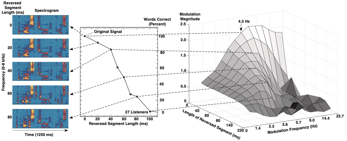
Figure 8.3 Long description
Left Panel: The spectrograms of the reversed segment visually represent the frequency and time components of the audio signal. The frequency ranges from 0 to 80 and the time ranges from 1250 milliseconds. Middle Panel: A point line graph compares the percentage of words correct, which ranges from 0 through 100, with the reversed segment length which ranges from 0 through 100. It plots a declining line which originates at (0, 100) and terminates at (100, 0). Right Panel: A 3 D surface plot showing the effect of both the length of the reversed segment and the modulation frequency on the modulation magnitude. The plot shows that the modulation magnitude is highest for shorter reversed segments and lower modulation frequencies. The peak of the surface is at a reversed segment length of approximately 100 milliseconds and a modulation frequency of 4.5 Hertz.
8.8 Rhythm as a Linguistic Parser
There are other reasons to believe phonemic elements are not the only, or even the optimal, way to linguistically model the speech stream. From both an acoustic and a spectral perspective, the speech signal has been likened to “scrambled eggs” (Hockett, Reference Hockett1960) with respect to how phonemic elements unfold acoustically when displayed in 2-D or 2.5-D representations (e.g., a spectrogram). There is considerable overlap between contiguous segments with respect to their phonetic properties. It is indeed a challenge to pinpoint where a phonetic element ends and the following one begins, especially for syllable-medial (typically vocalic) constituents (Greenberg, Reference Greenberg, Greenberg and Ainsworth2006). Rhythmic properties may facilitate the delineation of phonetic elements within a syllable by highlighting onsets, codas, and the interstitial nuclei.
The phonetic quality of a consonantal segment is heavily influenced by a variety of linguistic factors, the most important being its position within the syllable (e.g., onset, nucleus, coda), the syllable’s degree of prominence/stress (high, mid, low), and its approximate “place of articulation” (front, center, back of the oral cavity). The interaction of such features is what (mostly) determines how a consonant is phonetically realized within a syllable (Greenberg, Reference Greenberg, Greenberg and Ainsworth2006). Vocalic segments are sensitive to such factors as well, but their phonetic expression differs from consonants in that intensity, duration, and vowel height are the most relevant features. Vowels are more intense, longer, and lower in tongue height in highly prominent syllables than their less prominent counterparts (Greenberg et al., Reference Greenberg, Carvey, Hitchcock and Chang2003; Cho, Reference Cho2005).
8.9 Speech, Rhythm, and the Brain
How this parsing, analysis, and recoding are performed within the brain is not well understood. This is where speech rhythm is likely to play a prominent role, as it provides a sensory framework for low-frequency acoustic modulation to interact with other modulatory signals such as visual speech cues. Such sensory modulation provides a gateway for accessing endogenous neural activity that modulates at comparable (low) frequencies and incorporates a variety of information useful for interpretating ambiguous acoustic signals (see Chapter 3).
Low-frequency neural rhythms (aka “oscillations”) have been long thought to play a role in the processing of spoken language (Lenneberg, Reference Lenneberg1967) and certain other behaviors (Buzsaki, Reference Buzsaki2006, Reference Buzsaki2021; Chapter 3). Such cortical oscillations have been recorded in the language areas of the brain (e.g., Meyer, Reference Meyer2018; Poeppel and Assaneo, Reference Poeppel and Assaneo2020; Greenberg, Reference Greenberg2022). Although the specific function(s) of “delta” (0.5 Hz–3.5 Hz), “theta” (3.5 Hz–7 Hz), “beta” (10 Hz–25 Hz), and “gamma” (25 Hz–60 Hz) oscillations remains controversial (Buzsaki, Reference Buzsaki2006, Reference Buzsaki2021), it has been proposed that such endogenous rhythms are involved with certain aspects of linguistic processing (e.g., Greenberg, Reference Greenberg2011; Ding et al., Reference Ding, Melloni, Zhang, Tian and Poeppel2016).
It is tempting to link various brain rhythms to the processing and interpretation of specific linguistic constituents based largely on temporal properties. The periodicity of theta rhythm (3.5–7 Hz) coincides with that of syllabic elements (140–300 ms) across languages (Ding et al., Reference Ding, Melloni, Zhang, Tian and Poeppel2016), while “beta” oscillations (10–25 Hz) are similar in duration to the typical phonetic segment (40–100 ms) (Ding et al., Reference Ding, Melloni, Zhang, Tian and Poeppel2016). And the ultra-low-frequency “delta” waves (0.5 Hz–3.5 Hz) are comparable in length to spoken phrases and sentences (300 ms–2,000 ms). However, it’s unlikely the brain operates in such a rigid, lockstep fashion as some have proposed (e.g., Ghitza, Reference Ghitza2011).
Speech rhythm is often realized via certain modulatory properties of the signal. Prominent syllables are generally more intense than their less prominent counterparts (Greenberg et al., Reference Greenberg, Carvey, Hitchcock and Chang2003), which typically precede or follow them. This variation in amplitude (or “voice intensity”) helps pinpoint the most informative parts of the utterance to aid the listener’s parsing and interpretation of the communication (Greenberg, Reference Greenberg2022), especially helpful in adverse listening conditions (Assman and Summerfield, Reference Assmann, Summerfield, Greenberg, Ainsworth, Fay and Popper2004). The most prominent (i.e., highly stressed) syllables are longer in duration than their more lightly or unstressed counterparts, and such patterning is reflected in the modulation spectrum by a pronounced peak between 3 Hz and 6 Hz (Greenberg et al., Reference Greenberg, Carvey, Hitchcock and Chang2003, Figure 4). Shorter, less prominent syllables are represented in the modulation spectrum with energy in the 7 Hz to 12 Hz range.
8.10 Rhythmic-Centric Representations
It is widely acknowledged that such prosodic features as syllable prominence, stress accent, and phrasal intonation are as (if not more) important for linguistic communication than the classic notion of the phoneme. This is because prosody can influence the phonetic realization of much of what’s spoken (e.g., Greenberg, Reference Greenberg, Greenberg and Ainsworth2006). It also plays an outsized role in heavily emotional speech where certain syllables are often emphasized (aka hyper-articulation) to ensure the listener truly gets the speaker’s point (Lindblom, Reference Lindblom, Hardcastle and Marchal1990).
It has been hypothesized that the root cause of certain communication disorders may lie in neural timing issues as evidenced in deviant patterns of brain oscillations (Giraud and Poeppel, Reference Giraud and Poeppel2012; Leong and Goswami, Reference Leong and Goswami2014; Ding et al., Reference Ding, Melloni, Zhang, Tian and Poeppel2016, Reference Ding, Patel and Chen2017).
Models of spoken (and possibly written) language would likely benefit from integrating articulatory, acoustic, visual, and motor features into a unified theoretical framework that focuses on the interaction among different sources of linguistic information (e.g., McQueen and Dilley, Reference McQueen, Dilley, Gussenhoven and Chen2020). Such a unified perspective could aid in the development of new (and hopefully more efficacious) methods for teaching children to read and speak effectively (Leong and Goswami, Reference Leong and Goswami2014), as well as provide more effective ways of treating and ameliorating communication disorders impacting so many across their lifespan.
8.11 Acknowledgements
I thank the following colleagues for collaborating on research mentioned in this article: Takayuki Arai, Hannah Carvey, Shuangyu Chang, Oded Ghitza, Jeff Good, Ken Grant, Leah Hitchcock, Joy Hollenback, Brian Kingsbury, Nelson Morgan, and Rosaria Silipo. I would also like to thank reviewers Bettina Braun and Ting Huang for their helpful suggestions for improving this chapter. Thanks, as well, to the organizers of this special volume, Lars Meyer, Antje Strauss, and Caroline Duchow. Some of the material in this chapter was presented on March 12, 2021, at a virtual workshop in memory of John Ohala, organized by John Kingston and Didier Demolin.
Summary
Slow modulation of the acoustic speech signal plays a critical role in a listener’s ability to decode and comprehend spoken language. This low-frequency (3 Hz–16 Hz) rhythmic patterning derives from an interaction of articulatory processes with information-encoding imperatives shielding linguistic elements from adverse acoustic conditions common in the real world.
Implications
Models of spoken language often focus on phonemic elements as key building blocks of lexical meaning. A prosodic perspective, incorporating rhythm and syllabic prominence as central features, provides a more comprehensive foundation for understanding how listeners decode the speech signal, especially in adverse listening environments.
Gains
A prosodic, rhythmic model of spoken language understanding provides a theoretical foundation for investigating the neural bases of spoken and written language. Low-frequency (3 Hz–25 Hz) cerebral oscillations offer potential insight into the neurological bases of linguistic behavior, in particular how listeners go from sound to meaning.
9.1 Introduction
Whether speech is rhythmic is a controversial topic (Arvaniti, Reference Arvaniti2009; Goswami and Leong, Reference Goswami and Leong2013; Turk and Shattuck-Hufnagel, Reference Turk and Shattuck-Hufnagel2013; see Chapter 11). On the one hand, listeners tend to feel that speech is rhythmic and linguists have divided languages into syllable-timed and stress-timed languages, in which the syllable or stress is perceived to have regular rhythm (Dauer, Reference Dauer1983). On the other hand, no study has revealed strict periodicity in any speech unit or feature (Turk and Shattuck-Hufnagel, Reference Turk and Shattuck-Hufnagel2013; see Chapter 14). Therefore, the rhythm of speech cannot arise from strict periodicity in sound features or linguistic units. Since speech is a highly complex signal, the rhythm of speech can be discussed at multiple levels (see Chapter 20 for a discussion of the prosodic hierarchy of speech). Here, we consider the rhythm of three linguistic levels, that is, phones, syllables, and words. Furthermore, we only analyze the duration of a single unit or the interval between the onsets of neighboring units, instead of higher-order rhythms defined by the patterning of the onset of multiple units. The phone is the basic phonetic unit of speech, which can be further divided into vowels and consonants. A syllable typically contains one vowel that may be preceded and/or followed by a few consonants. Phones and syllables are units of speech sound, while morphemes and words are the basic units of meaning. A morpheme is the linguistically defined smallest unit for meaning (Boey, Reference Boey1975). A word is the basic unit for writing in some languages, such as English, but it is less well defined in other languages, such as Chinese (Tan and Perfetti, Reference Tan, Perfetti, Leong and Tamaoka1998).
In the last couple of decades, the rhythm of syllables has received a lot of attention. It is shown that syllables have a relatively regular duration, and the mean rate of syllables is typically between 4 and 8 Hz (Coupé et al., Reference Coupé, Oh, Dediu and Pellegrino2019; Greenberg et al., Reference Greenberg, Carvey, Hitchcock and Chang2003; Pellegrino et al., Reference Pellegrino, Coupé and Marsico2011; see Chapter 8). Furthermore, it is suggested that syllables have a relatively reliable acoustic correlate, that is, the speech envelope (Assaneo and Poeppel, Reference Assaneo and Poeppel2018; Cummins, Reference Cummins2012; Giraud and Poeppel, Reference Giraud and Poeppel2012; see also Zhang et al., Reference Zhang, Zou and Ding2023a, for different opinions). The speech envelope refers to the low-frequency (mainly below 30 Hz) changes in acoustic power, and its power spectrum, referred to as the modulation spectrum, peaks between 4 and 8 Hz, corresponding to the mean rate of syllables (Ding et al., Reference Ding, Patel and Chen2017; Greenberg et al., Reference Greenberg, Carvey, Hitchcock and Chang2003). Therefore, the rhythm of syllables, which is roughly equivalent to the rhythm of the speech envelope, can be perceived even without extensive linguistic knowledge, compared with the rhythm of phones (Liberman et al., Reference Liberman, Shankweiler, Fischer and Carter1974; see Chapter 11) or words, which requires learning. Although a number of studies have demonstrated that syllables have relatively regular duration, the statistical regularity of the duration of other linguistic units such as phones and words has seldom been investigated. Here, we analyzed the duration of phones, syllables, and words, and tested whether syllables have more regular duration than phones and words. We analyzed two languages that have the most users, Chinese and English.
9.2 Methods
9.2.1 Corpus
Eight speech corpora included in this analysis (Table 9.1) were extracted from six speech datasets, that is, DARPA-TIMIT (Garofolo et al., Reference Garofolo, Lamel and Fisher1993), GigaSpeech (Chen et al., Reference Chen, Chai and Wang2021), TED-LIUM (Rousseau et al., Reference Rousseau, Deléglise and Estève2012), Chinese-TIMIT (Yuan et al., Reference Yuan, Ding, Liao, Zhan and Liberman2017), Aishell-1 (Bu et al., Reference Bu, Du, Na, Wu and Zheng2017), and WenetSpeech (Zhang et al., Reference Zhang, Lv and Guo2022). The selection and processing of the corpora followed a recent study on the syllabic rhythm of speech (Zhang et al., Reference Zhang, Zou and Ding2023a).
| Corpus | Language | Speaking style | Total duration (h) |
|---|---|---|---|
| DARPA-TIMIT | English | Read sentences | 0.9 |
| GigaSpeech (audiobook) | English | Read audiobooks | 168.9 |
| TED-LIUM | English | Talk | 172.9 |
| GigaSpeech(interview) | English | Interviews | 40.8 |
| Chinese-TIMIT | Chinese | Read sentences | 5.8 |
| AISHELL-1 | Chinese | Read sentences | 179 |
| WenetSpeech (audiobook) | Chinese | Read audiobooks | 23.9 |
| WenetSpeech (talk) | Chinese | Talk | 54.3 |
9.2.2 Phone Duration
The boundaries of each phone (Figure 9.1) are automatically extracted based on audio and transcription using the Montreal Forced Aligner (MFA) (McAuliffe et al., Reference McAuliffe, Socolof, Mihuc, Wagner and Sonderegger2017). The MFA locates the boundaries between phones with a resolution of 10 ms; that is, the phone duration can only be a multiple of 10 ms. The MFA does not allow phones to overlap in time. This MFA method is validated based on the corpora for which manual labels of phone boundaries are available (Zhang et al., Reference Zhang, Zou and Ding2023a). The duration of a phone is defined as the time difference between phone onset and phone offset. The stimulus onset asynchrony (SOA) of phones is defined as the time difference between the onsets of two adjacent phones. The SOA is affected by the silence period after a phone, but the phone duration is not.
Schematized steady states and fast transit intervals.
The speech waveform and the boundaries of words, syllables, and phones.

9.2.3 Syllable Duration
The MFA also provides the boundaries between words for English and the boundaries between characters for Mandarin Chinese. In Chinese, since each syllable corresponds to a character, the syllable boundaries are obtained directly from the character boundaries. In English, the syllable boundaries (Figure 9.1) are determined by grouping the phones of each word into syllables based on a dictionary, that is, the Unisyn Lexicon (Fitt, Reference Fitt2001). The duration and SOA of syllables are defined in the same way they are for phones.
9.2.4 Duration of Theta Syllables
The structure of a syllable has three parts, that is, the onset, the nucleus/peak, and the coda/offset (Greenberg, Reference Greenberg1999). In general, the nucleus corresponds to the local maximum in speech intensity within the duration of a syllable. In the neuroscience literature, the concept of a theta syllable has also been proposed, which is the unit between two successive vocalic nuclei (Ghitza, Reference Ghitza2013). The concept is proposed to describe the units that are tracked by theta-band neural activity during speech listening. In connected speech, consonants may be produced in between two vowels, and parsing the boundaries of syllables requires determining which consonants are the offset of the first syllable and which consonants are the onsets of the second syllable. This syllable parsing problem is especially challenging for languages that allow flexible syllable structures, for example, English, compared with languages that have a highly regular syllable structure, for example, Turkish (Durgunoğlu and Öney, Reference Durgunoğlu and Öney1999). For theta syllables, however, the consonants between vowels do not need to be parsed into an onset and an offset. Here, we also analyze the statistical regularity in the duration of theta syllables.
9.2.5 Word Duration
For English, word boundaries (Figure 9.1) are reported by the MFA. For Chinese, words are not separated in the writing system, and there is no univocal definition of words. Here, word segmentation is achieved using a popular word segmentation tool, that is, stanza (Qi et al., Reference Qi, Zhang, Zhang, Bolton and Manning2020). The duration and SOA of words are defined in the same way they are for phones.
9.3 Statistical Distribution of Phones, Syllables, and Words
9.3.1 Mean Duration and SOA
In the following, for each language, Chinese and English, we report the results that are pooled across corpora, while the results of individual corpora are summarized in Table 9.2. For Chinese, the mean durations for phones, syllables, and words are 98 ms, 213 ms, and 327 ms, respectively. For English, the mean durations for phones, syllables, and words are 83 ms, 211 ms, and 294 ms, respectively. For phones, when vowels and consonants are separately analyzed, the duration of vowels (106 ms for Chinese and 89 ms for English) is slightly longer than the duration of consonants (91 ms for Chinese and 80 ms for English – Table 9.3). When comparing syllables and theta syllables, the mean duration is longer for theta syllables (231 ms for Chinese and 232 ms for English) than for syllables (213 ms for Chinese and 211 ms for English – Table 9.4). As expected, the SOA of a unit is longer than its duration (Table 9.2). For Chinese, the mean SOAs for phones, syllables, and words are 107 ms, 231 ms, and 353 ms, respectively. For English, the mean SOAs for phones, syllables, and words are 90 ms, 226 ms, and 317 ms, respectively (Table 9.2). The SOA for vowels is not shown, but it is the same as the duration of theta syllables reported in the subsequent analysis (Table 9.4).
| Duration | SOA | ||||
|---|---|---|---|---|---|
| Corpus | Unit | M ± SD (ms) | CV | M ± SD (ms) | CV |
| DARPA-TIMIT | phone | 80 ± 45 | 0.56 | 80 ± 45 | 0.57 |
| syllable | 205 ± 110 | 0.54 | 206 ± 111 | 0.54 | |
| word | 312 ± 191 | 0.61 | 313 ± 191 | 0.61 | |
| GigaSpeech (audiobook) | phone | 90 ± 52 | 0.58 | 94 ± 68 | 0.73 |
| syllable | 232 ± 126 | 0.54 | 243 ± 150 | 0.62 | |
| word | 316 ± 188 | 0.6 | 330 ± 214 | 0.65 | |
| TED-LIUM | phone | 78 ± 53 | 0.68 | 86 ± 88 | 1.02 |
| syllable | 194 ± 119 | 0.61 | 213 ± 169 | 0.8 | |
| word | 276 ± 191 | 0.69 | 309 ± 258 | 0.83 | |
| GigaSpeech (interview) | phone | 81 ± 59 | 0.72 | 88 ± 86 | 0.98 |
| syllable | 205 ± 122 | 0.6 | 222 ± 164 | 0.74 | |
| word | 281 ± 184 | 0.65 | 305 ± 226 | 0.74 | |
| Chinese-TIMIT | phone | 89 ± 39 | 0.43 | 92 ± 48 | 0.52 |
| syllable | 197 ± 60 | 0.3 | 203 ± 74 | 0.36 | |
| word | 307 ± 138 | 0.45 | 316 ± 150 | 0.47 | |
| AISHELL-1 | phone | 108 ± 57 | 0.53 | 114 ± 86 | 0.76 |
| syllable | 238 ± 77 | 0.32 | 251 ± 121 | 0.48 | |
| word | 376 ± 173 | 0.46 | 395 ± 206 | 0.52 | |
| WenetSpeech (audiobook) | phone | 91 ± 54 | 0.6 | 106 ± 109 | 1.03 |
| syllable | 192 ± 87 | 0.45 | 224 ± 158 | 0.71 | |
| word | 272 ± 166 | 0.61 | 313 ± 230 | 0.74 | |
| WenetSpeech (talk) | phone | 81 ± 51 | 0.64 | 93 ± 105 | 1.13 |
| syllable | 167 ± 83 | 0.5 | 192 ± 156 | 0.81 | |
| word | 252 ± 154 | 0.61 | 285 ± 218 | 0.77 | |
Note: M = mean duration in milliseconds; SD = standard deviation; CV = coefficient of variation
| Duration | |||
|---|---|---|---|
| Corpus | Unit | M ± SD (ms) | CV |
| DARPA-TIMIT | vowel | 89 ± 50 | 0.57 |
| consonant | 74 ± 40 | 0.54 | |
| GigaSpeech (audiobook) | vowel | 97 ± 61 | 0.62 |
| consonant | 86 ± 45 | 0.53 | |
| TED-LIUM | vowel | 81 ± 60 | 0.74 |
| consonant | 76 ± 47 | 0.62 | |
| GigaSpeech (interview) | vowel | 89 ± 71 | 0.79 |
| consonant | 76 ± 49 | 0.64 | |
| Chinese-TIMIT | vowel | 89 ± 43 | 0.49 |
| consonant | 89 ± 34 | 0.38 | |
| AISHELL-1 | vowel | 120 ± 64 | 0.53 |
| consonant | 97 ± 49 | 0.51 | |
| WenetSpeech (audiobook) | vowel | 95 ± 63 | 0.66 |
| consonant | 87 ± 46 | 0.52 | |
| WenetSpeech (talk) | vowel | 81 ± 60 | 0.74 |
| consonant | 80 ± 43 | 0.54 | |
| Corpus | Duration | |
|---|---|---|
| M ± SD (ms) | CV | |
| DARPA-TIMIT | 204 ± 106 | 0.52 |
| GigaSpeech (audiobook) | 241 ± 147 | 0.61 |
| TED-LIUM | 227 ± 188 | 0.83 |
| GigaSpeech (interview) | 224 ± 170 | 0.76 |
| Chinese-TIMIT | 201 ± 72 | 0.36 |
| AISHELL-1 | 247 ± 120 | 0.49 |
| WenetSpeech (audiobook) | 229 ± 164 | 0.72 |
| WenetSpeech (talk) | 197 ± 153 | 0.78 |
9.3.2 Coefficient of Variation (CV)
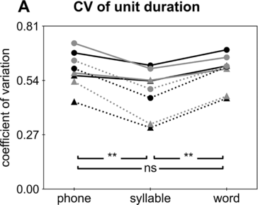
The CV is a measure of relative variability, calculated as the ratio of the standard deviation to the mean. A lower CV indicates stronger statistical regularity. For the duration/SOA of a unit, a lower CV indicates stronger rhythmicity. For duration, the CV of syllables (0.39 for Chinese and 0.57 for English) is consistently lower than the CV of phones (0.55 for Chinese and 0.64 for English; binomial test based on the results from the eight corpora, p < 0.01) and the CV of words (0.54 for Chinese and 0.64 for English; see Table 9.2 and Figure 9.2A; binomial test, p < 0.01). For SOA, the CV of syllables (0.59 for Chinese and 0.67 for English) is significantly lower than the CV of phones (0.86 for Chinese and 0.82 for English; binomial test, p < 0.01) and words (0.62 for Chinese and 0.71 for English; binomial test, p < 0.05), while the CV of words is significantly lower than the CV of phones (Table 9.2; Figure 9.2B; binomial test, p < 0.05).
CV.
CV for unit duration. Each line shows the CV of a corpus. Chinese and English corpora are marked out by dots and triangles, respectively. Pairwise comparisons between phones, syllables, and words are carried out using the binomial test (* p < 0.05, ** p < 0.01).
CV for SOA.

9.4 The Rate of Phones, Syllables, and Words
In the neurolinguistic literature, the rate of a linguistic unit is more frequently discussed than the duration/SOA of a unit. The rate of a unit, however, can be defined in several ways. First, it can be defined as the total number of units divided by the total duration of speech recordings. This definition is the same as the reciprocal of the mean SOA of the unit, denoted as 1/E(SOA) in this chapter. The rate defined this way is sensitive to the duration of silence periods in the recording, which can be problematic if the recording has long silence periods. To solve this problem, the second definition excludes the silence periods in speech and defines the rate of a unit as the total number of units in a corpus divided by the total duration of units. For this definition, the rate of a unit is simply the reciprocal of the mean unit duration, denoted as 1/E(duration) in this chapter. A third definition is, for the duration of each unit, take the reciprocal and calculate the mean of this reciprocal. This measure is denoted as E(1/duration) in this chapter.
The rates of phones, syllables, and words calculated using these three methods are summarized in Table 9.5. When the units were pooled over all corpora, the rates for phones, syllables, and words calculated using method 1, that is, 1/E(SOA), are 10.4 Hz, 4.4 Hz, and 3.0 Hz, respectively. For method 2, that is, 1/E(duration), the rates for phones, syllables, and words are 11.3 Hz, 4.7 Hz, and 3.3 Hz, respectively. The rate calculated using method 1 is lower than the rate calculated using method 2 since it considers the silence period after a unit. For the third measure, that is, E(1/duration), the rates for phones, syllables, and words are 15.1 Hz, 6.3 Hz, and 5.0 Hz, respectively, higher than the rates calculated using the other two methods. The result is expected, since 1/E(1/duration) is the harmonic mean of duration, which is more strongly influenced by small values than the arithmetic mean, that is, E(duration), and the harmonic mean is always smaller than the arithmetic mean.
| Corpus | Unit | 1/E(SOA) | 1/E(duration) | E(1/duration) |
|---|---|---|---|---|
| DARPA-TIMIT | phone | 12.50 | 12.54 | 17.30 |
| syllable | 4.86 | 4.88 | 6.73 | |
| word | 3.19 | 3.21 | 5.16 | |
| GigaSpeech (audiobook) | phone | 10.62 | 11.10 | 14.44 |
| syllable | 4.12 | 4.31 | 5.76 | |
| word | 3.03 | 3.17 | 4.68 | |
| TED-LIUM | phone | 11.68 | 12.84 | 17.28 |
| syllable | 4.70 | 5.16 | 7.41 | |
| word | 3.35 | 3.75 | 6.93 | |
| GigaSpeech (interview) | phone | 11.36 | 12.32 | 17.15 |
| syllable | 4.51 | 4.89 | 6.90 | |
| word | 3.28 | 3.55 | 5.53 | |
| Chinese-TIMIT | phone | 10.90 | 11.24 | 13.58 |
| syllable | 4.92 | 5.08 | 5.70 | |
| word | 2.66 | 2.74 | 3.76 | |
| AISHELL-1 | phone | 8.79 | 9.29 | 11.83 |
| syllable | 3.98 | 4.21 | 4.72 | |
| word | 2.10 | 2.20 | 2.84 | |
| WenetSpeech (audiobook) | phone | 9.46 | 11.03 | 14.93 |
| syllable | 4.47 | 5.21 | 6.57 | |
| word | 2.79 | 3.20 | 4.85 | |
| WenetSpeech (talk) | phone | 10.81 | 12.42 | 16.66 |
| syllable | 5.20 | 6.00 | 7.78 | |
| word | 3.06 | 3.46 | 5.13 |
9.5 Discussion
Rhythmicity in speech has motivated theoretical and experimental studies on how neural oscillations encode speech. Although such neuroscientific research is flourishing, relatively few studies have empirically characterized the rhythmicity in speech (Ding et al., Reference Ding, Patel and Chen2017; Inbar et al., Reference Inbar, Grossman and Landau2020; Meyer, Reference Meyer2018; Meyer et al., Reference Meyer, Henry, Gaston, Schmuck and Friederici2016; Stehwien and Meyer, Reference Stehwien and Meyer2022; Tilsen and Arvaniti, Reference Tilsen and Arvaniti2013; Zhang et al., Reference Zhang, Zou and Ding2023a; see more in Chapter 16). The rhythmicity of speech, however, is the basis for these neuroscientific studies and therefore deserves more attention. Here, we investigated the mean and variation of the duration of phones, syllables, and words, since the duration information of these units has been used to motivate hypotheses and analysis approaches in neuroscientific studies on speech processing (Coopmans et al., Reference Coopmans, de Hoop, Hagoort and Martin2022; Giraud and Poeppel, Reference Giraud and Poeppel2012; Kaufeld et al., Reference Kaufeld, Bosker and ten Oever2020; Kazanina and Tavano, Reference Kazanina and Tavano2022; Keitel et al., Reference Keitel, Gross and Kayser2018; ten Oever et al., Reference ten Oever, Carta, Kaufeld and Martin2022; Zhang et al., Reference Zhang, Zou and Ding2023b).
Since a word contains one or more syllables and a syllable contains one or more phones, for the three levels of units, the mean duration is longest for words and shortest for phones. The nesting relationship between the three units, however, does not decide which unit has stronger rhythmicity, and the empirical analyses here show that syllables have a statistically significantly lower CV of duration than phones and words, indicating that syllables have more regular duration. Although the difference is statistically significant, the CV of phone/word duration is only about 1.3 times bigger than the CV of syllable duration (Table 9.2). The difference is small compared to the variation of CV across speech corpora that differ in their language or speaking style. For example, the syllable CV tends to be lower for Chinese than for English, indicating higher syllabic rhythmicity for Chinese than for English. Even for the Chinese corpora, the syllable CV is lower for read sentences, that is, Chinese-TIMIT and AISHELL, than for spontaneous speech, that is, WenetSpeech (talk).
Roughly speaking, the mean rates for phones, syllables, and words fall into the range of alpha, theta, and delta oscillations, respectively. The mean rate of phones, however, does not contradict the hypothesis that gamma-band oscillations are critical for the neural encoding of phones (Giraud and Poeppel, Reference Giraud and Poeppel2012; Goswami, Reference Goswami2016; Hovsepyan et al., Reference Hovsepyan, Olasagasti and Giraud2020; Hyafil et al., Reference Hyafil, Fontolan, Kabdebon, Gutkin and Giraud2015; Meyer, Reference Meyer2018), since the hypothesis focuses on the critical timescales within a phone, for example, the timescales for formant transitions and voicing, instead of the mean rate of phones.
Summary
We quantified the statistical regularity in the duration of phones, syllables, and words. The CV is below 0.7 for the three units for most corpora, suggesting that the unit duration is relatively regular. Furthermore, the CV is slightly lower for syllables than for phones and words and is highly variable across corpora.
Implications
According to the mean rate of phones, syllables, and words, if some neural activity can track the onset of each phone, syllable, or word, its frequency will fall into the range of alpha, theta, and delta oscillations, respectively.
Gains
Phones, syllables, and words all have their typical duration. Future studies may also probe how phone, syllable, and word rates vary across speakers, and whether these rhythms are steady or show systematic variations over time.
10.1 Introduction
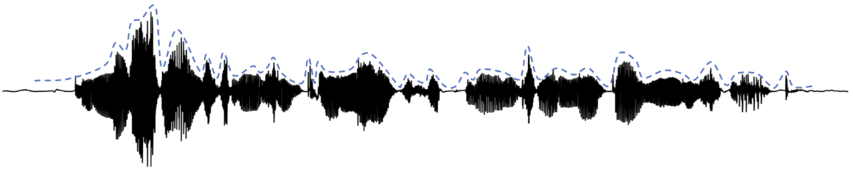
The analysis of amplitude envelopes has become a widespread method in the speech sciences (Gibbon, Reference Gibbon2021; Mermelstein, Reference Mermelstein1975; Rosen, Reference Rosen1992), language acquisition research (Goswami, Reference Goswami2018, Reference Goswami2019), and neurolinguistics (Assaneo et al., Reference Assaneo, Ripolles and Orpella2019; Gross et al., Reference Gross, Hoogenboom and Thut2013; Obleser et al., Reference Obleser, Herrmann and Henry2012; Poeppel, Reference Poeppel2014; Poeppel and Assaneo, Reference Poeppel and Assaneo2020). Loosely speaking, amplitude envelopes capture the amplitude distribution over the waveform of an utterance; a common metaphor is that their shape is like a blanket put over a waveform such that the individual positive glottal spikes “carry” the blanket. High-energy sounds (vowels, but also some sonorants and sibilants) lead to bumps in the amplitude envelopes; low-energy sounds (non-sibilant fricatives, stops) lead to troughs, as visualized in Figure 10.1. These amplitude envelopes present a low-frequency time-varying signal.
Schematic display of amplitude envelope.
Waveform (black) with a stylized amplitude envelope (dashed line) shifted upwards to increase visibility.
Like for any other signal, one can extract the spectrum of the low-frequency amplitude envelope, which gives an indication of the frequencies of modulation that have the most direct association with the concept of speech rhythm. Three reasons make the analysis of amplitude envelopes and modulation frequencies (i.e., modulation spectra) interesting. First, envelopes capture the part of the signal that is relevant to convey rhythm, which makes them a prime candidate for a fresh look at acoustic research on speech rhythm (Arvaniti, Reference Arvaniti2009, Reference Arvaniti2012; Barry, Reference Barry, Trouvain and Gut2007; Ramus et al., Reference Ramus, Nespor and Mehler1999), beyond the analysis of durational cues (Dauer, Reference Dauer1983) and acoustic isochrony. Second, the method is easy to apply to speech, without manual annotation. Third, it has been proposed that neural oscillations at different frequency bands track linguistic structure in speech, such as phonemes or syllables (Assaneo et al., Reference Assaneo, Ripolles and Orpella2019; Gross et al., Reference Gross, Hoogenboom and Thut2013; Poeppel, Reference Poeppel2014).
Despite the increasingly widespread use across disciplines, there is little research on which aspects of speech influence the amplitude envelopes in what ways. Cross-linguistic comparisons suggest that a language’s rhythm affects the modulation spectra in particular (see Section 10.3.1). The aim of this chapter is twofold: It first provides an acoustic and statistical overview of previous studies (Section 10.2); then it reviews some literature on modulation spectra for linguistic contrasts at the phrase level (Section 10.3: cross-linguistic differences, speaking styles, and illocution type) and more locally at the word level (Section 10.4: the role of segmental length and pitch accent type). Where possible, we provide data of our own, analyzed with the same workflow to allow for comparison of the magnitude of the differences (as a measure of effect size) and the frequency bands at which linguistic contrasts exert their differences (to allow for generalizations and the generation of hypotheses for future studies). Of the five linguistic contrasts included in this chapter, pitch accent type is the only one that does not alter the general rhythmic structure of an utterance (irrespective of accent type, the pitch accent is associated with the very same word; pitch accents primarily consist of frequency modulations, not amplitude modulations; see Gibbon, Reference Gibbon2021). Pitch accent type is hence not expected to change the amplitude envelopes and serves as a perfect control condition to probe the specificity of the procedure for capturing rhythmic aspects. The chapter closes with an overview of the effect sizes and frequency domains in which effects are located for the own data (presented in Sections 10.3.1, 10.3.3, 10.4.1, and 10.4.2), discusses potential generalizations, and postulates desiderata for future research (Section 10.5).
This contribution focuses on the interpretation of amplitude envelopes in terms of phonetic and linguistic factors. Adhering to the book’s scope, it primarily covers research that investigates aspects that pertain to speech rhythm. Hence, it does not cover the neurolinguistic literature that is concerned with testing links between brain oscillations and modulation frequencies of the amplitude envelope (see Chapters 3 and 5). Amplitude envelopes share some overlap with research on perceptual centers (p-centers; see Marcus, Reference Marcus1981; Rathcke et al., Reference Rathcke, Lin, Falk and Dalla Bella2021) and amplitude rise times, which are related to vowel onsets (Chapter 11). This literature is, however, not covered here.
10.2 Acoustic and Statistical Background
Low-pass-filtered amplitude envelopes capture the slow-varying energy distributions over the course of an utterance. Technically, modulations can be extracted in different ways (for a comparison between extraction techniques and their relation to vowel onset, see MacIntyre et al., Reference MacIntyre, Cai and Scott2022). A common procedure is to filter the spectrum into a range of bands (between 70 Hz and 10,000 Hz). The cutoff points for filtering are either spaced logarithmically or equidistantly on the cochlear map (Chandrasekaran et al., Reference Chandrasekaran, Trubanova, Stillittano, Caplier and Ghazanfar2009; Gross et al., Reference Gross, Hoogenboom and Thut2013; Todd and Brown, Reference Todd and Brown1994; Varnet et al., Reference Varnet, Ortiz-Barajas, Erra, Gervain and Lorenzi2017). The initial decomposition of the signal into bands has the advantage of representing amplitude information from different frequency bands, information that has been shown to affect intelligibility (see Chapter 8) because the different frequency bands provide information on an utterance’s linguistic structure (Assaneo et al., Reference Assaneo, Ripolles and Orpella2019; Gross et al., Reference Gross, Hoogenboom and Thut2013; Poeppel, Reference Poeppel2014). The envelope itself can be extracted using half-wave rectification (making the signal positive) followed by low-pass filtering (Caetano and Rodet, Reference Caetano and Rodet2011; Gibbon, Reference Gibbon2021; Kolly and Dellwo, Reference Kolly and Dellwo2014; Loizou et al., Reference Loizou, Dorman and Tu1999) or by using the Hilbert transform (Braiman et al., Reference Braiman, Fridman and Conte2018; MacIntyre et al., Reference MacIntyre, Cai and Scott2022; O’Sullivan et al., Reference O’Sullivan, Power and Mesgarani2015). These two methods are said to achieve largely similar results (Ding et al., Reference Ding, Patel and Chen2017, p. 182). The wideband envelope is derived by the sum of the narrowband envelopes (Chandrasekaran et al., Reference Chandrasekaran, Trubanova, Stillittano, Caplier and Ghazanfar2009) or their average (Varnet et al., Reference Varnet, Ortiz-Barajas, Erra, Gervain and Lorenzi2017). Other authors do not initially decompose the signal into frequency bands but first band-pass-filter the signal (e.g., between 400 and 4,000 Hz) and then low-pass-filter it (<10 Hz), for example, by using Butterworth filters (Tilsen and Johnson, Reference Tilsen and Johnson2008).
In most cases, researchers analyze amplitude envelopes spectrally, that is, in the frequency domain. To that end, modulation frequencies are extracted by discrete Fourier transform (Gibbon, Reference Gibbon2021; Tilsen and Johnson, Reference Tilsen and Johnson2008). The result is a spectrum, that is, a continuous power curve across frequency bands. The signal typically follows a 1/f trend; that is, it has the highest energy in low-frequency bands (note that this 1/f trend is removed in some approaches). The different frequencies relate to linguistic units of different sizes (phrasal rate: 0.6–1.3 Hz; word/stress rate: 1.8–3 Hz; syllable rate: 4–5 Hz; phone rate: 8–10 Hz [Keitel et al., Reference Keitel, Gross and Kayser2018]). One metric that is employed is the frequency of the highest peak (when the 1/f trend is removed), which is consistent across languages (Ding et al., Reference Ding, Patel and Chen2017; Varnet et al., Reference Varnet, Ortiz-Barajas, Erra, Gervain and Lorenzi2017) and related to the syllable rate (but see Zhang et al., Reference Zhang, Zou and Ding2023). Other researchers analyze the envelope in the time domain using empirical mode decomposition of the amplitude modulation (Tilsen and Arvaniti, Reference Tilsen and Arvaniti2013) and extract different parameters from that signal. Some authors combine measures from both the frequency and the time domains (Lau et al., Reference Lau, Patel and Kang2022). It is clear that the variety of signal-processing methods makes it hard to directly compare results and effect sizes across studies. For the analysis of our own data presented here (specifically in Sections 10.3.1, 10.3.3, 10.4.1, and 10.4.2), we used nine gammatone frequency bands between 100 and 10,000 Hz, spaced equidistantly on the cochlear map, followed by low-pass filtering of the rectified narrowband signals. These narrowband envelopes were summed to derive a wideband envelope, which was then submitted to Fourier analysis (see Einfeldt and Braun, Reference Einfeldt, Braun, Skarnitzl and Volín2023 and Frota et al., Reference Frota, Vigário, Cruz, Hohl and Braun2022, for more details on these methods). Neither the sound files nor the amplitude envelope modulation spectra were normalized (i.e., the 1/f trend was not removed).
There are different kinds of analyses of amplitude envelopes in the literature. One approach has been to correlate aspects of the amplitude modulation spectra with visual phonetic information (Chandrasekaran et al., Reference Chandrasekaran, Trubanova, Stillittano, Caplier and Ghazanfar2009, with mouth-opening data), acoustic information (MacIntyre et al., Reference MacIntyre, Cai and Scott2022, with acoustic vowel onsets; Varnet et al., Reference Varnet, Ortiz-Barajas, Erra, Gervain and Lorenzi2017, with temporal rhythm metrics such as pairwise variability indices), or phonological information (Gibbon, Reference Gibbon2021, with morphophonological information; Leong and Goswami, Reference Leong and Goswami2015, with feet, syllables, and onset–rime units; Todd and Brown, Reference Todd and Brown1994, with the phonological stress hierarchy of a word). It has also been tested how useful the amplitude envelope information is for prediction (Ludusan et al., Reference Ludusan, Origlia and Cutugno2011: prominent syllables; MacIntyre et al., Reference MacIntyre, Cai and Scott2022: vowel onsets) and clustering (Gibbon, Reference Gibbon2021). In studies that investigate effects of particular factors on the amplitude modulation spectra, mixed-effects models (Baayen et al., Reference Baayen, Davidson and Bates2008) or general additive mixed models (GAMMs) have been employed (Wood, Reference Wood2006). For our own data presented here (see Sections 10.3.1, 10.3.3, 10.4.1, and 10.4.2), we used GAMMs as they allow the researcher to model differences in power across frequency bands in a continuous manner, while accounting for autocorrelation (see Frota et al., Reference Frota, Vigário, Cruz, Hohl and Braun2022, for details of the statistical modeling). GAMMs establish the frequency bands in which significant differences occur across conditions and can be used for both exploratory and hypothesis-testing research questions. They allow for a statistic comparison of effect sizes (differences in log power, mathematically equivalent to ratios of raw power) and frequency bands across conditions.
10.3 Cross-linguistic and Cross-stylistic Comparisons
10.3.1 Cross-linguistic Comparisons
In linguistics, languages have been grouped into different rhythm classes (stress-timed, syllable-timed, mora-timed) based initially on perceptual impression. A common assumption is that there is a roughly equal distance between the respective linguistic units. Since such isochrony (typically established by annotation of segments) has been difficult to establish (e.g., Chapter 14; Dauer, Reference Dauer1983), other composite metrics have been suggested (see Grabe and Low, Reference Grabe, Low, Gussenhoven and Warner2002; Ramus et al., Reference Ramus, Nespor and Mehler1999), all relying on manual annotation. However, these measures are also not without difficulties (Arvaniti, Reference Arvaniti2009, Reference Arvaniti2012), and the analysis of low-frequency amplitude envelopes is expected to support cross-linguistic differences in speech rhythm. Interestingly, there are a number of studies that suggest that amplitude envelopes have globally similar shapes across languages, including peaks in power for low-modulation frequencies followed by a decrease in amplitude (Ding et al., Reference Ding, Patel and Chen2017; Poeppel and Assaneo, Reference Poeppel and Assaneo2020; Varnet et al., Reference Varnet, Ortiz-Barajas, Erra, Gervain and Lorenzi2017). One of the most comprehensive studies was conducted by Ding et al. (Reference Ding, Patel and Chen2017). They analyzed amplitude modulations from nine different languages (American English, British English, Chinese, Dutch, Danish, French, German, Norwegian, and Swedish). Their analyses show a peak in the (1/f-corrected) speech modulation spectrum around 4 Hz, independent of (the rhythm of the) languages. Varnet et al. (Reference Varnet, Ortiz-Barajas, Erra, Gervain and Lorenzi2017) analyzed semi-spontaneous productions from 10 languages (Basque, Dutch, English, French, Japanese, Marathi, Polish, Spanish, Turkish, and Zulu). They showed that the amplitude envelopes differed between stress-timed and syllable-timed languages (p. 1981). Frota et al. (Reference Frota, Vigário, Cruz, Hohl and Braun2022) compared amplitude envelopes in three rhythmically different languages: stress-timed German, and more syllable-timed Brazilian and European Portuguese. They showed that rhythmic differences across languages are reflected in modulation spectra: stress-timed German had higher power than more syllable-timed Brazilian and European Portuguese in the delta (1–2 Hz) and theta bands (6–8 Hz). European and Brazilian Portuguese also differed, but only in the delta band (1–2 Hz), with similar mean differences as between German and the two Portuguese varieties. The difference between the two Portuguese varieties may be due to macro-rhythmic difference (see Jun, Reference Jun2012): There are more frequent pitch accents in Brazilian than European Portuguese, affecting the energy distribution over the utterance, which is then picked up in the low-frequency amplitude envelope. Tilsen and Arvaniti (Reference Tilsen and Arvaniti2013) compared six languages (English, German, Greek, Italian, Korean, and Spanish) (see Section 10.3.2 for more detail). Their cross-linguistic analysis showed that English differed from the other languages, but no other comparisons were significant. The special characteristics of English were explained in terms of the “relatively high degree of supra-syllabic periodicity in English and minimal differences among the other languages in the corpus” (p. 635). In sum, Varnet et al. (Reference Varnet, Ortiz-Barajas, Erra, Gervain and Lorenzi2017) and Frota et al. (Reference Frota, Vigário, Cruz, Hohl and Braun2022) reported differences between stress-timed and syllable-timed languages, while Ding et al. (Reference Ding, Patel and Chen2017) and Tilsen and Arvaniti (Reference Tilsen and Arvaniti2013) did not. Possible reasons for discrepancies in outcomes are differences in the type and amount of materials (read sentences versus longer texts and more spontaneous productions; see Section 10.3.2) or differences in the type of signal processing.
10.3.2 Speaking Styles
The most rhythmic style analyzed in the literature is probably English nursery rhymes spoken in synchrony to a metronome in infant-directed speech (Leong and Goswami, Reference Leong and Goswami2015). But also, quite generally, infant-directed speech showed a higher amplitude in the delta band (around 2 Hz) than adult-directed speech (Leong et al., Reference Leong, Kalashnikova, Burnham and Goswami2017), suggesting a clearer foot-based rhythm. In their cross-linguistic study introduced in Section 10.3.1, Tilsen and Arvaniti (Reference Tilsen and Arvaniti2013) further tested for effects of speaking styles (spontaneous speech, read sentences, read passages). They showed an effect of speaking style on time domain aspects of the speech envelopes, distinguishing spontaneous speech from the two read speech recordings (p. 635).
10.3.3 Illocution Type
Hohl and Braun (Reference Hohl and Braun2023) tested the influence of illocution type, in particular whether a question was meant as an information-seeking or a rhetorical one. This contrast can be signaled lexically – see (1) versus (2) – but also by means of prosody.
(1)
What time is it? information-seeking question (2)
Who likes paying taxes? rhetorical question
Prior analyses have shown that rhetorical questions are realized with longer constituent durations than information-seeking questions (Braun et al., Reference Braun, Dehé, Neitsch, Wochner and Zahner2019; Dehé and Braun, Reference Braun, Dehé, Neitsch, Wochner and Zahner2019, Reference Dehé and Braun2020). Furthermore, they were more often realized with a breathy voice quality (in particular in German) and differed in global intonation. In English polar questions, moreover, participants often shifted the accent from the default accent on the final noun in information-seeking questions (e.g., Does anyone like lemon?) to the indefinite in rhetorical questions (e.g., Does anyone like lemon? [small capitals signal accent location]). The analyses of amplitude envelopes showed differences across illocution types in all languages. The strongest difference (0.5 log power) was observed for English between 3.1 and 4.7 Hz (with larger power for rhetorical than for information-seeking questions). Further smaller differences were present between 1.4 and 1.9 Hz. Icelandic showed differences in slightly lower frequency bands (0.5–1.2 Hz and 3.4–3.8 Hz), but of a smaller magnitude than English (0.2 log power with large variability). The magnitude of the differences for German lay in between (0.4 log power), but occurred in a higher frequency band (7.3–9.1 Hz). The authors argued that the differential effects of illocution type in the three languages cannot be explained by differences in segment durations alone (which were overall largest in Icelandic and smaller in German and English) but must be caused by other differences. Likely predictors are accent placement (for English) and the use of a breathy voice in initial segments in rhetorical questions (in German). We will return to this in the General Discussion (Section 10.5).
10.4 Local Differences in Segmental Length and Pitch Accent Type
10.4.1 Segmental Length
In languages with segmental length contrasts, the length of segments (vowels or consonants) distinguishes lexical candidates. It is expected that the different durations influence the “local” rhythmic structure of target words and hence the modulation spectra. Hohl et al. (Reference Hohl, Behrens-Zemek and Braun2022) extracted spectra for German word pairs differing in vowel length, which were matched for lexical frequency (e.g., Mitte [ˈmɪṫʰə] “center” versus Miete [ˈmiːtʰə] “rent”). Note that length in German is often, but not always, accompanied by vowel quality. The results showed that words with a long vowel had a lower power in a small frequency band just below 2 Hz and, importantly, between 5 and 8.5 Hz (mean difference of 0.4 in log power). Interestingly, the segmental length effect disappeared when the target words were embedded in carrier phrases (Das nächste Wort war XXX, “The next word was XXX”), suggesting that the effect of vowel length on the global rhythmic profile of utterances is negligible.
The effect of consonantal length in native speakers of Italian was studied in Einfeldt and Braun (Reference Einfeldt, Braun, Skarnitzl and Volín2023) (see top panel of Figure 10.2). In their first experiment, they extracted modulation spectra from six Italian speakers from 16 minimal pairs only differing in phonemic consonant length (e.g., fato [ˈfato] “fate” and fatto [ˈfatːo] “fact, done”). The results showed that the Italian consonantal length contrast is evident in a large frequency band in the modulation spectra. Compared to the German vowel length contrast, the Italian consonantal length contrast has power differences in a larger frequency interval (2–7.4 Hz compared to 5–8 Hz) and is larger in magnitude (up to 0.5 larger log power in geminates than in singletons). The most likely reason for these cross-linguistic differences in magnitude and frequency band between Italian consonantal and German vocalic length is that the Italian length contrast is distributed over a longer temporal interval, with adjustments to not only the duration of the consonant but with complementary temporal adjustment in the preceding vowel (Payne, Reference Payne1995) and even the word-initial consonant (Turco and Braun, Reference Turco and Braun2014).
Differences in amplitude envelope spectra for two linguistic contrasts.
Estimated effects of consonantal length in Italian (top) and pitch accent type in German (bottom), as predicted by the GAMM model (left panel) and estimated differences (right panel). The gray band shows the 95% CI of the difference.
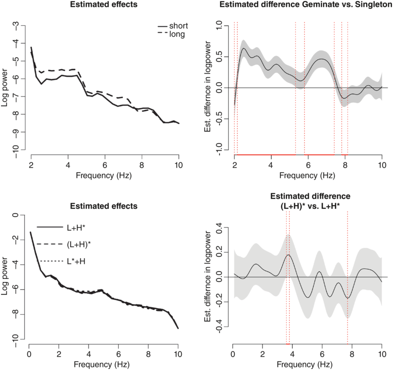
Figure 10.2 Long description
Top left. A line graph of log power ranging from minus 3 through minus 10 versus a frequency that ranges from 2 through 10 hertz. The graph plots a solid line for short consonants (Singleton) which originates from (2, minus 4), declines and terminates at (10, minus 8.5) and a dotted line for long consonants (Geminate), which is higher than the solid line in certain frequency bands. Top right. A line graph compares the estimated difference in log power between two conditions, namely, Geminate and Singleton across different frequency bands. It plots a fluctuating line along with the shaded area the represents the confidence interval. Bottom left. A line graph compares the log power with the frequency. It plots an overlapping line which represents L plus H star, LH star and L star plus H The line originates at approximately at (0, minus 1.5), declines, and terminates at (10, minus 9). Bottom right. A line graph compares the estimated difference in log power between two conditions across frequency bands. It plots a fluctuating line with the shaded area that represents the confidence interval.
10.4.2 Pitch Accent Type
So far, there has been little information in the literature as to whether/how pitch accent type (i.e., rising or falling) directly affects the amplitude envelope. The data used for testing this factor was originally collected in Zahner-Ritter et al. (Reference Zahner-Ritter, Einfeldt and Wochner2022). The study tested three conditions that differed in the alignment of the low and high tonal targets with respect to the stressed syllable in rising–falling accents. In L+H*, the low (L) tone preceded the stressed syllable while the high (H) tone was aligned with the stressed syllable; in (L+H)*, both the low and the high tonal targets were aligned with the stressed syllable; and in L*+H, the low tone was aligned with the stressed syllable and the high tone in the following syllable. Since a change in accent shape (on the same word) does not have a strong influence on an utterance’s rhythm, we do not expect an effect of intonation condition on the amplitude modulation spectra. The data hence serve as a control condition to test the specificity of the modulation spectra for rhythmic contrasts.
For the purpose of this chapter, we analyzed the modulation spectra of imitation data from native German speakers who imitated the three-way accent contrast in rising–falling accents on words in wh-questions (e.g., Wer malt denn mandalas? “Who draws PRT mandalas”). The results of the GAMM analysis showed an improvement in the modal fit when adding a random smooth for accent over a model without that random smooth term (χ2(6) = 6903.6, p < 0.0001). However, the estimated effects of the three accents overlap to a large degree (see Figure 10.2, left panel). Pairwise comparisons between the three kinds of accentual realizations showed only minimal differences in power for one of the accent contrasts: There was slightly higher power in (L+H)* than L+H* in the frequency range between 3.6 and 3.8 Hz. The mean difference in power was 0.2, with a lot of variability (95% CI [confidence interval] of the difference: [0.01;0.38]; see bottom panel of Figure 10.2). It is possible that the model picked up on the higher energy exerted by producing a salient rise in the stressed syllable compared to shallower rises in L+H* and L*+H accents. In any case, the effects of fundamental frequency (f0) contour are minimal.
10.5 General Discussion
This chapter provided an overview of the extraction and analysis methods of amplitude envelope modulations in the literature. It then focused on the role of some linguistic factors that may affect the rhythmic structure of utterances: rhythm class, speech style and illocution, as well as segmental length. As a control condition, to test the specificity of the method for capturing rhythmic contrasts, we added an analysis of the effect of pitch accent type on amplitude envelopes. As expected, this factor only marginally affected the amplitude envelope modulation spectra (in a very small frequency band and with little difference in power), supporting the view that amplitude envelopes carry first and foremost rhythmic information.
The different aspects examined here had different effects on the amplitude envelopes, both in terms of the magnitude of the (log) power differencesFootnote 1 and of the frequency bands that were affected: The largest mean differences across conditions were observed for different rhythm classes (macro rhythm: Brazilian versus European Portuguese; stress timing versus syllable timing: German versus Portuguese), followed by consonantal length in minimal pairs in Italian, and rhetorical versus polar questions in English (mean differences > 0.5). The other linguistic factors had smaller effects (rhetorical versus information-seeking questions in German and Icelandic, differences in vowel length in German) (see Table 10.1). Pitch accent type, the control condition, showed very small effects with a large spread.
Overview of differences in amplitude modulation spectra (frequency bands, maximum frequency range of significant differences Δf) and maximum differences in log power (including the 95% CI of the difference) for selected linguistic contrasts, analyzed with the same method, ordered by decreasing maximum mean difference in log power. (EP: European Portuguese; BP: Brazilian Portuguese).
| Contrast | Frequency bands of significant differences (Hz) | Max Δf (Hz) | Max. mean difference | 95% CI of difference |
|---|---|---|---|---|
| Macro rhythm (EP vs. BP) Stress timing (German) vs. syllable timing | 1.3–2.5 G vs. EP: 1.4–1.8; 6.7–9.3 G vs. BP: 1.6–2.4; | 1.2 2.6 1.0 | 0.7 0.6 0.6 | [0.5;1.0] [0.5;1.0] [0.4;1.0] |
| 7–7.9; 9–10 | ||||
| Consonant length | 2–7.4 | 5.4 | 0.6 | [0.5;0.7] |
| English rhetorical vs. information-seeking questions | 1.4–1.9; 3.1–4.7 | 0.5 | 0.5 | [0.35;0.65] |
| Vocalic length | 2.1–3.8 | 1.7 | 0.4 | [0.1;0.6] |
| German rhetorical vs. information-seeking questions | 7.3–9.1 | 1.8 | 0.35 | [0.15;0.55] |
| Icelandic rhetorical vs. information-seeking questions | 0.5–1.2; 3.4–3.8 | 0.7 | 0.3 | [0.15;0.45] |
| Pitch accent type | (L+H)* vs. L+H*: 3.6–3.8 | 0.2 | 0.2 | [0.01; 0.4] |
Differences in the lowest frequency bands (0.5–2.5 Hz) are observed for rhythm class (macro rhythm, stress timing versus syllable timing) as well as English and Icelandic rhetorical versus information-seeking questions (roughly in the range between), that is, aspects that concern the whole utterance. However, differences in the highest frequency bands (> 7.3 Hz) are also caused by phrasal aspects (stress timing versus syllable timing, German rhetorical versus information-seeking questions). This is surprising given that these frequency bands capture phone-sized units (Keitel et al., Reference Keitel, Gross and Kayser2018). We conclude that rhythm class and illocution type exert influence on a segmental level as well, which is then tracked in these higher frequency bands. The more local length contrasts had different effects: vowel length in the vicinity of the syllable rate (around 4 Hz), consonant length in a very broad frequency band. This is consistent with the observation that the consonantal length contrast is not limited to the duration of the respective consonant but is distributed more widely. The effect of the control condition, pitch accent type, was minimal.
In terms of the size of affected frequency intervals, Italian consonantal length exerted effects in the largest frequency range (Δ = 5.4 Hz; see Table 10.1). Pitch accent type, on the other hand, had differences in the smallest frequency range (Δ = 0.2 Hz). This latter finding strengthens the conclusion that differences in pitch accent type alone do not alter the amplitude envelope (or the rhythmic structure).
For future research, it would be desirable to provide access to off-the-shelf, open-source programs, such that results across languages and factors become more comparable across labs. In terms of the signal processing involved, application-oriented researchers may benefit from mathematically easier methods (e.g., low-pass filtering compared to Hilbert transform) because they can be more readily understood and results may find a broader audience.Footnote 2
Carefully controlled materials provide a useful first step to target the linguistic aspects that influence low-frequency amplitude envelopes. This will ideally lead to a model from which we can derive testable predictions for future research and for analyzing more heterogeneous speech materials. To date, it clearly seems that (macro-)rhythmic differences across languages as well as consonantal length have a robust influence in the low-frequency range (around 2 Hz). Studies from more languages are needed to test the generalizability of this finding.
10.6 Acknowledgements
I thank Friederike Hohl, Hendrik Behrens-Zemek, and Marieke Einfeldt for recording participants and pre-processing data. Thanks are further due to Volker Dellwo for providing the script to extract the narrowband envelopes, to Sonia Frota and Antje Strauß for general discussion about low-frequency amplitude envelopes and cross-linguistic differences, to Anna Verebély for help with figure quality, and to Dafydd Gibbon for valuable comments on an earlier version.
Summary
After an introduction to amplitude envelopes, the chapter compared several linguistic contrasts (rhythm class, speaking style, consonantal and vocalic length, pitch accent type) with regards to their respective effects on amplitude envelope modulation spectra. Results showed the largest power differences for rhythm class and the smallest differences for pitch accent type.
Implications
Amplitude envelopes provide a holistic measure that efficiently captures rhythmic differences. The comparison of controlled data allowed us to isolate different factors and work towards a model of factors that influence amplitude envelopes. Future research will benefit from more languages and the provision of transparent open-source scripts to ease comparison.
Gains
Neurobiology has long thought of links between amplitude envelopes in the speech signal and brain oscillations. The current research allows us to better understand the links between linguistic factors and the amplitude envelope, ultimately leading to a model that describes the connections between linguistic units and brain oscillations.
11.1 The Perceptual Center in Speech
The notion of the perceptual center (or the P-center) dates back to the beginnings of speech rhythm research that focused on temporal isochrony (Morton et al., Reference Morton, Marcus and Frankish1976), though the concept has not lost its appeal to the present day (Lin and De Jong, Reference Lin and De Jong2023; Zoefel et al., Reference Zoefel, Gilbert and Davis2023). The P-center is defined as the subjectively perceived moment of occurrence, highlighting that acoustic and perceptual onsets of rhythmic events do not necessarily co-occur (Morton et al., Reference Morton, Marcus and Frankish1976). Instead, the P-center seems to lag behind the acoustic onset of the corresponding rhythmic event, such as a (monosyllabic) word. The discovery was made with a recording of English digits from one to nine that were evenly concatenated to create an isochronous rhythmic sequence. The evenly spaced concatenation, however, sounded irregular to the experimenters (and other listeners). The sequence could only be made regular once the digits were concatenated with reference to the perceived, rather than acoustic, isochrony (Morton et al., Reference Morton, Marcus and Frankish1976). It was observed that the perceptual onsets of the concatenated digits deviated systematically, but somewhat inconsistently, from their acoustic counterparts. They did not coincide with local peaks in signal amplitude or fundamental frequency (Morton et al., Reference Morton, Marcus and Frankish1976).
Figure 11.1 illustrates this idea with the recording of a speaker producing the words bad, mad, sad, had, ad, pad at a steady pace as cued by a 2.5 Hz metronome (with an interval of 400 ms between beat onsets). If we measure the resulting intervals between successive word onsets, the produced sequence of words is irregular. And yet it sounds isochronous, just as the speaker intended to produce it. Under the P-center view, perceptual isochrony of this example derives from an even spacing of the P-centers of rhythmic speech events. The concept has also been applied to music (London et al., Reference London, Nymoen and Langerød2019; Vos and Rasch, Reference Vos and Rasch1981), and some discussions of the P-center propose that it constitutes the level of the beat in speech, thus linking the rhythmic structure of speech and music (Allen, Reference Allen1972; Cumming et al., Reference Cumming, Wilson, Leong, Colling and Goswami2015; Harsin, Reference Harsin1997; Harsin and Green, Reference Harsin and Green1994; Hoequist, Reference Hoequist1983; Scott, Reference Scott1998). The beat in music is defined as an underlying grid of equal time intervals that provides temporal structure to musical notes (Savage et al., Reference Savage, Brown, Sakai and Currie2015). It is uncontroversially regular in contrast to speech timing that shows no evidence for isochrony and very limited evidence for regularity (Arvaniti, Reference Arvaniti2009; Dauer, Reference Dauer1983; Rathcke and Smith, Reference Rathcke and Smith2015), at least on the surface of measurable acoustics (Turk and Shattuck-Hufnagel, Reference Turk and Shattuck-Hufnagel2013). The P-center effect indicates that equal time intervals may exist in speech after all, and that they are perceptual rather than acoustic in nature.
Illustration of the P-center effect.
The word sequence consisting of six English words (bad, mad, sad, had, ad, and pad) was produced in sync with a metronome at 2.5 Hz (or 400 ms between beat onsets) and sounds highly regular. However, the resulting inter-onset intervals between successive word onsets vary between minimally 312 ms (mad-sad) and maximally 534 ms (had-ad), demonstrating a discrepancy between (irregular) acoustics and (regular) perception typical of the P-center effect.

11.2 Methods of Examining the P-Center
Following its discovery, the P-center was extensively researched using a great variety of methods with the ultimate goal of developing an algorithm that would automatically identify P-center location in speech. One method gave rise to the example shown in Figure 11.1. In this task, participants are asked to produce a series of words or syllables in time with a (real or imagined) metronome (e.g., Chow et al., Reference Chow, Belyk, Tran and Brown2015; Fowler, Reference Fowler1979; Fox and Lehiste, Reference Fox and Lehiste1987a; Marcus, Reference Marcus1981; Šturm and Volín, Reference Šturm and Volín2016; Tuller and Fowler, Reference Tuller and Fowler1980). The subsequent analyses focus either on determining the alignment point of the metronome beat and the speech signal or on identifying the magnitude of discrepancies between timings of words with identical versus varied phonological structure. Another commonly used task is based on the perceptual adjustment for isochrony (e.g., Cooper et al., Reference Cooper, Whalen and Fowler1988; Harsin, Reference Harsin1997; Marcus, Reference Marcus1981; Pompino-Marschall, Reference Pompino-Marschall1989; Scott, Reference Scott1998). In a version of this task, listeners are given one base word repeating with a fixed inter-onset interval and asked to adjust the timing of a following, phonologically different word such that it matches the regular inter-onset intervals of the preceding base word repetitions. The subsequent analyses of listeners’ adjustments examine temporal deviations between the inter-onset intervals established by the base words and the perceptually matched words that deviate from the base word in their phonological structure. Another variant of the task asks listeners to align words to metronome beats (Pompino-Marschall, Reference Pompino-Marschall1989). Finally, participants have also been asked to tap along with a designated syllable of a looped sequence of words (Allen, Reference Allen1972). The timing of the tap can then be analyzed, determining the location of the syllable’s P-center.
Having discovered the P-center effect with a series of isolated monosyllabic words, Morton et al. (Reference Morton, Marcus and Frankish1976: 405) were cautious to add that the properties (and the existence) of the P-center may well be “subject to phonological, semantic, or syntactic influences” that play a role in natural speech. These influences have not yet been empirically addressed (see Chapter 22). While it has also been suggested that the P-center effect may explain the apparent lack of isochrony in speech acoustics (e.g., Lehiste, Reference Lehiste1977; Morton et al., Reference Morton, Marcus and Frankish1976), no studies have examined the P-center in connected speech. Across all methods mentioned above, speech materials consist of isolated, real or nonce, words presented with an intervening pause. The materials can be varied with regards to the identity of onset consonants and the phonological complexity on their clusters (e.g., seed, bead, lead, blead), the vowel quality in the syllable nucleus (e.g., bad, bed, bid), the presence or absence of coda consonants, and the complexity of codas (e.g., see, seek, seeks), but they have been generally restricted to mono- or bisyllabic words. Evidence from related work on beat perception in natural connected speech indicates that the subjectively perceived onset of the beat in spoken sentences indeed deviates from the acoustic onset of phonological syllables (Lin and Rathcke, Reference Lin and Rathcke2020; Rathcke et al., Reference Rathcke, Lin, Falk and Dalla Bella2021), providing preliminary support for the P-center effect in speech of higher complexity than one-word utterances (though without demonstrating an isochronous distribution of P-centers in natural speech).
11.3 On the Location of the P-Center
There is no generally accepted model of the exact P-center location (Villing et al., Reference Villing, Repp, Ward and Timoney2011). The evidence on which factors affect it and in what ways is mixed. It is mostly assumed to lie somewhere close to the vowel onset (Barbosa et al., Reference Barbosa, Arantes, Meireles and Vieira2005; Franich, Reference Franich2018; Hoequist, Reference Hoequist1983; Marcus, Reference Marcus1981) and to be mostly affected by syllable onsets rather than codas (Howell, Reference Howell1988; Marcus, Reference Marcus1981; Pompino-Marschall, Reference Pompino-Marschall1989; Scott and Howell, Reference Scott and Howell1992; Šturm and Volín, Reference Šturm and Volín2016), though these generalizations may be limited to Germanic and possibly Romance languages that have predominantly been studied to date (Šturm and Volín, Reference Šturm and Volín2016). In Cantonese, however, monosyllabic words produced in time with a metronome do not show the tendency for the beat to lag behind the acoustic syllable onset (Chow et al., Reference Chow, Belyk, Tran and Brown2015). The speech-to-metronome synchronization in this tonal language is tightly timed to syllable-initial consonants rather than vowels (Chow et al., Reference Chow, Belyk, Tran and Brown2015), casting doubts on the existence of the P-center in Cantonese and, more generally, on the effect being a cross-linguistic universal as previously suggested (Hoequist, Reference Hoequist1983).
Overall, the effect has been documented in nontonal languages including English (e.g., Cooper et al., Reference Cooper, Whalen and Fowler1988; Fowler, Reference Fowler1979; Fox, Reference Fox1987; Harsin, Reference Harsin1997; Tuller and Fowler, Reference Tuller and Fowler1980), German (Pompino-Marschall, Reference Pompino-Marschall1989; Pompino‐Marschall et al., Reference Pompino‐Marschall, Kühnert and Tillmann1989), Brazilian Portuguese (Barbosa et al., Reference Barbosa, Arantes, Meireles and Vieira2005), Spanish (Hoequist, Reference Hoequist1983), Czech (Šturm and Volín, Reference Šturm and Volín2016), and Japanese (Fox, Reference Fox1987; Hoequist, Reference Hoequist1983). Extending typological diversity, the effect has recently been ascertained in Medumba, a tonal language of the Bantu family (Franich, Reference Franich2018), and Mandarin Chinese (Lin and De Jong, Reference Lin and De Jong2023). This finding suggests that the lack of the P-center effect in Cantonese cannot be due to lexical tone. Chow et al. (Reference Chow, Belyk, Tran and Brown2015) explain their result with reference to syllable structure in Cantonese whose onsets are either empty or occupied by one or maximally two (an obstruent plus a glide) consonants. The authors suggest that the phonotactic restriction may have the acoustic consequence that the prevocalic part in Cantonese syllables is relatively short and minimally variable, leading to vowel onsets being less reliable acoustic landmarks than onsets of syllable-initial consonants. However, the syllable structure of Cantonese is quite comparable to that of Japanese (Kubozono, Reference Kubozono1989; Otake et al., Reference Otake, Hatano, Cutler and Mehler1993), yet Japanese speakers (Hoequist, Reference Hoequist1983) and listeners (Fox, Reference Fox1987) display the P-center effect in production and perception comparable to the one found with English speakers and listeners. Moreover, Mandarin Chinese has an even more restricted syllable phonotactics than Cantonese (e.g., Zhao and Berent, Reference Zhao and Berent2016), though a recent production study indicates that the P-center of Mandarin Chinese is located close to the acoustic vowel onset, just as in nontonal languages. Language-specific syllable phonotactics is thus less likely to be the main reason for the cross-linguistic differences in the P-center effect.
While Cantonese boasts a complex tone system with several dynamic and level tones, Medumba has a two-way contrast (Franich, Reference Franich2018) and Mandarin has a four-way contrast (Lin and De Jong, Reference Lin and De Jong2023). It is unclear whether this difference in tonal inventory can account for the discrepancy in P-center findings across the three tonal languages. It is also unclear whether pitch plays any role in influencing the location of the P-center. While Chow et al. (Reference Chow, Belyk, Tran and Brown2015) did not observe any differences between P-centers of Cantonese words carrying different tones and Lin and De Jong (Reference Lin and De Jong2023) only examined syllables with tone-1, Franich (Reference Franich2018) measured differently timed P-centers in words carrying a low versus high tone, with high tones leading to earlier P-centers. In their seminal study, Morton et al. (Reference Morton, Marcus and Frankish1976) did not find an effect of pitch on P-center location in English. This finding was confirmed in a recent study with more complex English materials (Lin and Rathcke, Reference Lin and Rathcke2020; Rathcke and Lin, Reference Rathcke and Lin2023), though there remains a possibility that pitch may shape beat perception in some (not necessarily tonal) languages.
In languages that clearly demonstrate the P-center, its location seems to be affected by the properties of the whole syllable or word, though the effects of onset, nucleus, and coda are neither similar in magnitude nor additive, and the evidence documenting the (phonological versus phonetic) nature of P-center shifts is mixed. Early work by Marcus (Reference Marcus1981) experimented with natural and manipulated versions of monosyllabic words for English digits and found that their P-center was located later in the syllable if the duration of the onset was shorter, or if the vowel or coda duration was longer. Fox and Lehiste (Reference Fox and Lehiste1987a) asked if such durational influences on P-center shifts were phonological rather than phonetic in nature, given that many phonological contrasts (e.g., tense versus lax vowels in English) go hand in hand with timing alternations (long versus short). They conducted a study into the effect of vowel quality as opposed to vowel duration on P-center location, examining English monosyllables with lax versus tense vowel nuclei. The results indicated little role of vowel phonology in shifting the location of the P-center within a syllable, confirming that the nature of the P-center effect was purely phonetic rather than phonological. An opposite conclusion was reached by Šturm and Volín (Reference Šturm and Volín2016) who demonstrated that P-center location in bisyllabic words of Czech was strongly affected by the phonological vowel length rather than their phonetic duration.
Cooper et al. (Reference Cooper, Whalen and Fowler1986) studied the phonetic influence of syllable onsets and nuclei by varying the duration of fricative noise in a fricative-vowel syllable, the duration of acoustic silence in a fricative-stop-vowel syllable, or the duration of the vowel itself. The perception of the P-center in the resulting stimuli was mostly affected by the duration of the syllable-initial consonant(s) and, to a lesser extent, by the duration of the vowel, showing temporal shifts similar to those documented by Marcus (Reference Marcus1981). Following up on this work, Cooper et al. (Reference Cooper, Whalen and Fowler1988) examined the role of syllable rime in more detail, testing the hypothesis put forward by Marcus (Reference Marcus1981) that the rime behaves as a unit such that durational variability in the vowel versus the coda does not exert an independent influence on the location of the P-center. Two experiments systematically manipulated the duration of the vowel in a vowel-consonant syllable with either covarying or constant duration of the rime. The results did not provide evidence in support of the hypothesis by Marcus (Reference Marcus1981). Instead, they suggested that both constituents of the rime (i.e., vowels and codas) had comparable effects on affecting P-center location.
A series of experiments with more varied materials conducted by Pompino-Marschall (Reference Pompino-Marschall1989), however, showed that the phonetic effects of segment duration on P-center location were not as linear and additive as suggested by earlier research. Rather, the duration of the syllable onset, vowel, and coda interacted in complex ways, jointly determining the direction and the magnitude of shifts in P-center location. Adding to this complexity, Harsin (Reference Harsin1997) provided further evidence that the durational effect of syllable onsets on P-center location did not equally apply across a wide range of consonants but was moderated by the phonological category of the onset. Specifically, syllables with sonorants versus obstruents of the same duration differed in their P-centers and did not display a unified effect of consonant lengthening on a later location of the P-center that had been generally shown in earlier work with more limited materials (Allen, Reference Allen1972; Cooper et al., Reference Cooper, Whalen and Fowler1988; Fowler, Reference Fowler1979; Marcus, Reference Marcus1981). Given that sonorants and obstruents show remarkable differences in their energy distributions and amplitude envelopes, subsequent work focused primarily on the attempts to model P-center location as a function of spectro-temporal properties of a syllable, even though experimental evidence to this end had been rather mixed (Harsin, Reference Harsin1997; Marcus, Reference Marcus1981; Morton et al., Reference Morton, Marcus and Frankish1976; Tuller and Fowler, Reference Tuller and Fowler1980).
Testing an acoustic account of the P-center in their original work, Morton et al. (Reference Morton, Marcus and Frankish1976) excluded local peaks in signal amplitude or in fundamental frequency as suitable signal-driven anchors of the center location. Subsequent studies further elaborated that the P-center did not coincide with any acoustic landmarks in speech (e.g., Cooper et al., Reference Cooper, Whalen and Fowler1986; Marcus, Reference Marcus1981). However, Howell (Reference Howell1988) and Scott and Howell (Reference Scott and Howell1992) revisited the acoustic account of the P-center and proposed a model based on the amplitude envelope and a syllabic “center of gravity,” suggesting that perceptual judgments are linked to the distribution of the energy in a syllable (see Chapter 3). In this model, the center of gravity refers to the moment when the energy peak of a syllable is reached, typically at the consonant-vowel transition. The slope of the energy rise toward the center of gravity is assumed to encode onset consonants and is crucial to the calculations of P-center location. If the energy contour rises quickly right from the syllable onset (as for some syllable-initial fricatives), the P-center occurs earlier; if it shows a more gradual increase, the P-center is located later (the concept came to be widely known as syllable rise time, e.g., Goswami et al., Reference Goswami, Fosker, Huss, Mead and Szűcs2011; Leong et al., Reference Leong, Hämäläinen, Soltész and Goswami2011). This model stands in contrast to the most recent acoustic representation of P-center location that somewhat downplays the energy of some consonants – notably fricatives – in order to derive the P-center (Šturm and Volín, Reference Šturm and Volín2016). According to Šturm and Volín (Reference Šturm and Volín2016), the P-center is best represented as the moment of the fastest energy change (maxD) occurring at the consonant-vowel transitions within a syllable, though for the algorithm to perform well, the high energy of some consonants such as fricatives ought to be significantly downplayed and smoothed (Šturm and Volín, Reference Šturm and Volín2016: 42). Previous attempts to localize the P-center at the midpoint of the amplitude rise time did not have that feature (Cummins and Port, Reference Cummins and Port1998). The two algorithms are available for researchers with an interest in the study of the P-center, either from the first author’s website (Cummins and Port, Reference Cummins and Port1998) or upon individual request (Šturm and Volín, Reference Šturm and Volín2016).
Despite some differences, both algorithms of P-center location operate within the domain of a syllable and sample acoustic properties of the local amplitude envelope delimited by the syllable boundaries. There is, however, some evidence that the P-center can also be affected by a preceding or following syllable. For example, Fox and Lehiste (Reference Fox and Lehiste1987b) showed that the P-center shifts to a later location if an additional syllable is suffixed to form a bisyllabic word. In contrast, it shifts (even more substantially) to an earlier location if an additional syllable is prefixed. While Šturm and Volín (Reference Šturm and Volín2016) focused specifically on bisyllabic words, they did not compare them to monosyllables, so it is unclear whether or not their maxD algorithm should account for polysyllabic complexity and in what ways. In recent work, we applied the algorithm to more varied and naturally complex materials in English and examined the potential of the maxD-derived landmark to predict the location of finger taps produced during a task requiring participants to synchronize with the beat of repeated sentences (Rathcke et al., Reference Rathcke, Lin, Falk and Dalla Bella2021). The results showed that the maxD landmark was statistically as good a predictor of finger-tap locations as vowel onsets. Even though both the task and the stimuli of this sensorimotor synchronization experiment by far exceeded the complexity of more traditional P-center paradigms, the findings confirmed that the P-center effect existed in the perception of rhythmic beat structure in natural English speech. That is, there is a discrepancy between the acoustic onset of a syllable and the perceived onset of the syllable beat.
11.4 Explanations of the P-Center Effect
The original interest in the effect was grounded in the idea that rhythm meant isochrony and motivated by the search for some temporal constancy in language. The discovery of the effect gave rise to the hypothesis that isochrony in language might be perceptual and not acoustic (Lehiste, Reference Lehiste1977; Morton et al., Reference Morton, Marcus and Frankish1976). Even though the idea that speech rhythm can be defined purely on the basis of duration and timing has received much criticism (Arvaniti, Reference Arvaniti2009; Kohler, Reference Kohler2009) and is not unanimously shared (White and Malisz, Reference White, Malisz, Gussenhoven and Chen2020), the P-center effect maintains its relevance to speech rhythm research as it signifies a notable discrepancy between speech acoustics and perception. Such discrepancy is not unique to the P-center but generally applies to a range of speech perception phenomena that show nonlinear relationships with physical input properties (e.g., Dilley and Pitt, Reference Dilley and Pitt2010; Goldstone and Hendrickson, Reference Goldstone and Hendrickson2010; Warren, Reference Warren1968).
As noted by Morton et al. (Reference Morton, Marcus and Frankish1976: 408), the concept of the P-center has “no explanatory power” of its own as it simply describes one temporal aspect of speech perception. Not surprisingly, approaches to explaining the origin of the P-center effect somewhat mirror approaches to understanding speech perception in general. A prominent account in this regard is the proposal put forward by Fowler and colleagues (Fowler, Reference Fowler1979, Reference Fowler1986, Reference Fowler1994; Tuller and Fowler, Reference Tuller and Fowler1980). It follows the motor theory of speech perception (Liberman and Mattingly, Reference Liberman and Mattingly1985), assuming that articulatory gestures constitute perceptual units in connected speech and that P-centers track the kinematic signal of speech production or, more specifically, the temporal regularity of vowel gestures (see Chapter 2). Accordingly, the P-center effect originates in the fact that “listeners extract information from the acoustic signal that specifies articulatory timing” (Fowler et al., Reference Fowler, Whalen and Cooper1988: 94). While articulatory recordings do not straightforwardly support the motor account of the P-center (De Jong, Reference De Jong1992, Reference De Jong1994; Pompino‐Marschall et al., Reference Pompino‐Marschall, Kühnert and Tillmann1989), the key suggestion that beat perception in speech may be locked to vowels is further found in other discussions of the P-center effect (Barbosa et al., Reference Barbosa, Arantes, Meireles and Vieira2005; Rathcke et al., Reference Rathcke, Lin, Falk and Dalla Bella2021). For example, Barbosa et al. (Reference Barbosa, Arantes, Meireles and Vieira2005) hypothesize that P-centers can best be understood as a surface manifestation of the perceptual task to predict upcoming vowel onsets in a sequence of syllables. Similarly, Rathcke et al. (Reference Rathcke, Lin, Falk and Dalla Bella2021) discuss that vowels have a special importance for speech perception as they shape the sonority contour of the acoustic speech signal. The resulting fluctuations in signal sonority may support speech segmentation and assist first-language acquisition (Räsänen et al., Reference Räsänen, Doyle and Frank2018). Naturally evolved drummed languages such as Amazonian Bora also make use of such sonority fluctuations and map rhythmic units onto intervocalic intervals (Seifart et al., Reference Seifart, Meyer, Grawunder and Dentel2018), further corroborating the special role of vowels for the perception of speech rhythm. In languages spoken around the world, the nucleus (most frequently occupied by a vowel) represents the only obligatory constituent of a syllable and is often reflected in a local sonority maximum (Blevins, Reference Blevins and Goldsmith1995).
Rathcke et al. (Reference Rathcke, Lin, Falk and Dalla Bella2021) also note that during rhythmic synchronization with the beat of natural sentences, it was particularly the very first vowel of a sentence that showed anticipation – in other words, a vowel occurring after an acoustic silence. All subsequent vowels – in other words, vowels embedded in a meaningful sentence – were synchronized with more precisely and in a less anticipatory way. Notably, previous studies of P-center location experimented with isolated words concatenated using silent pauses. It is therefore not implausible to hypothesize that the P-center may reflect a temporal prediction of a vowel onset that is expected to occur after a silent pause. This explanation of the P-center effect is in line with current evidence of negative mean asynchrony obtained in rhythmic synchronization tasks with a variety of auditory stimuli (Aschersleben, Reference Aschersleben2002; Repp and Su, Reference Repp and Su2013). Accordingly, measurable anticipation of regular auditory prompts occurs specifically when those prompts are interspersed with acoustic silences but is attenuated, or even completely removed, in complex, continuous rhythmic contexts such as music (see Chapter 6). This hypothesis of P-center origin requires experimental testing in future research.
Alternative accounts of the P-center assume that the effect is rather acoustic (Howell, Reference Howell1988; Scott and Howell, Reference Scott and Howell1992; Šturm and Volín, Reference Šturm and Volín2016; Vos and Rasch, Reference Vos and Rasch1981) or psychoacoustic (Harsin, Reference Harsin1993, Reference Harsin1997; Pompino-Marschall, Reference Pompino-Marschall1989) in nature. These accounts highlight that the P-center is neither unique to speech nor completely independent of the spectro-temporal features of the stimuli tested. Psychoacoustic models define P-centers with reference to critical-band audio frequency regions that matter for the human auditory system (see Chapter 3). Accordingly, the P-center effect arises due to a salient acoustic energy change within the critical audio frequency bands of an entire syllable. The P-center itself can then be best modeled as a tracker of acoustic changes at relevant frequencies to which a perceptual weighting function is applied. The weighting function integrates the knowledge of critical bands as well as perceptual thresholds that need to be reached for the P-center effect to arise at a given point in time.
Purely acoustic models tend to abstract away from the complexities of critical frequency bands and nonlocal influences on P-center location. These models see the origin of the effect in the perceptual system sampling amplitude envelopes at onsets of auditory input units (e.g., syllables, tones, or metronome clicks) and responding particularly sensitively to salient points of the maximal rate of change. Most recent installments of this account further suggest that the perceptual system may not be simply attracted to the local moments of the fastest energy change but is sensitive to the overall rate of change in the amplitude envelope (i.e., slope and rise time). Accordingly, only some acoustic signals lend themselves readily to the perception of a clear P-center at a certain point in time (Villing et al., Reference Villing, Repp, Ward and Timoney2011), while others may be perceived like a “broad slur” (Benadon, Reference Benadon2014). A notion of a “beat bin” has been put forward to account for the fact that the clarity of the P-center tends to vary across different types of auditory input (Danielsen et al., Reference Danielsen, Nymoen and Anderson2019), though this idea has not yet been comprehensively investigated, particularly in speech.
11.5 Unresolved Issues and Future Directions
Apart from the controversies surrounding the exact P-center location, difficulties with the development of suitable P-center algorithms, and limited availability of cross-linguistic evidence, the current understanding of the effect faces one key issue – individual variability. As Pompino-Marschall (Reference Pompino-Marschall1989) notes, listener performance in P-center tasks can differ rather substantially. Early work even reported on difficulties in determining P-center locations with inexperienced listeners (Cooper et al., Reference Cooper, Whalen and Fowler1988; Fox and Lehiste, Reference Fox and Lehiste1987b; Morton et al., Reference Morton, Marcus and Frankish1976). Several studies reviewed above are based on data from no more than three or four participants, which, in the presence of large individual variability, suggests that the difficulty in establishing P-center location may be even greater than currently appreciated, though it may also be more meaningful than currently assumed. Studying the P-center effect with a more representative sample of 23 Cantonese participants, Chow et al. (Reference Chow, Belyk, Tran and Brown2015: 63) also noted that the participants “behaved quite differently from one another.” The answer to the question of which individual listener traits and characteristics moderate the perceptual variability may potentially help to better explain the origins and the nature of the effect. Some preliminary findings indicate that musical training (or, more generally, musical aptitude) plays a role in rhythmic tasks such as P-center paradigms (Rathcke et al., Reference Rathcke, Lin, Falk and Dalla Bella2021; Šturm and Volín, Reference Šturm and Volín2016). Participants with higher levels of musical training show reduced variability of P-center responses (Šturm and Volín, Reference Šturm and Volín2016) and higher accuracy in rhythmic synchronization with vowel onsets (Rathcke et al., Reference Rathcke, Lin, Falk and Dalla Bella2021). Having studied the effect with highly skilled musicians, Villing et al. (Reference Villing, Repp, Ward and Timoney2011: 1626) found consistent results across a range of tasks and argued that P-centers demonstrated “a reliable and universal percept” – a conclusion that probably owed a lot to the homogeneity of the participating group of listeners.
However, the role of musical aptitude and training is possibly limited to the perception of participants whose native languages do not have lexical tone, as Chow et al. (Reference Chow, Belyk, Tran and Brown2015) did not observe any systematic differences in P-center location among musically trained and untrained Cantonese participants. Little is known if, and how, native language(s) of listeners shape(s) their beat perception in speech and other complex auditory signals, which is a fruitful avenue to explore in future studies of the P-center effect.
Summary
The P-center refers to the perceptual moment of occurrence of a speech unit and has been hypothesized to represent the beat in spoken language. It can be found among many other controversial concepts surrounding the idea of rhythm in speech and language. Over decades of study, the exact location and the nature of the P-center have remained largely unresolved, though the concept itself has retained its potential to inform future research.
Implications
The P-center effect has direct implications for the construction of speech stimuli, specifically for those experiments that work with concatenated monosyllables interspersed by silent pauses. If the P-center effect is not considered, an acoustically constant inter-onset interval connecting a string of phonologically variable monosyllables may be perceived as irregular, while a (slightly) jittered concatenation results in a good approximation of perceptual regularity.
Gains
The key contribution of the P-center to the current understanding of rhythm in speech and language is rather profound as it establishes that the perception of temporal structure in speech, just as the perception of spectral and other features, deviates from the acoustic signal in complex ways and is not universal but language-specific. As such, the P-center signifies that a purely acoustic study of speech rhythm is likely to be futile.
12.1 Introduction
The challenge of speech perception begins with the infinitely large space of possible messages, and is exponentially compounded by the infinite variations with which any one message can be transduced into an auditory signal. In practice, human listeners can tolerate incredible variability in speech signals, resulting from different content, speakers, and contexts (Miller and Licklider, Reference Miller and Licklider1950; Huggins, Reference Huggins1964; Beasley et al., Reference Beasley, Bratt and Rintelmann1980; Drullman et al., Reference Drullman, Festen and Plomp1994; Shannon et al., Reference Shannon, Zeng, Kamath, Wygonski and Ekelid1995; Dorman et al., Reference Dorman, Loizou and Rainey1997; Ahissar et al., Reference Ahissar, Nagarajan and Ahissar2001; Huang et al., Reference Huang, Chen, Li, Chang and Zhou2001; Ghitza and Greenberg, Reference Ghitza and Greenberg2009). At the same time, speech perception remains exquisitely sensitive to subtle variations in linguistic and paralinguistic signals, with listeners extracting nuanced information from a huge variety of cues (Munhall et al., Reference Munhall, Jones, Callan, Kuratate and Vatikiotis-Bateson2004; Mattys et al., Reference Mattys, White and Melhorn2005; Kurumada et al., Reference Kurumada, Brown, Bibyk, Pontillo and Tanenhaus2014; Baese-Berk et al., Reference Baese-Berk, Morrill and Dilley2018). How is it that listeners extract meaning from speech with a combination of robustness and sensitivity as yet unequaled by artificial speech recognition? The variability of speech provides a route to a solution, rather than posing an inherent problem, by providing rich context to shape the search space of possible interpretations. These perspectives connect to an emerging conceptual understanding of perception, action, and cognition as Bayesian inference, formalized by developments in the theory of hierarchical probabilistic generative models (Rao and Ballard, Reference Rao and Ballard1999; Knill and Pouget, Reference Knill and Pouget2004; Friston et al., Reference Friston, Kilner and Harrison2006, Reference Friston, Daunizeau and Kiebel2009; Adams et al., Reference Adams, Shipp and Friston2013; Millidge et al., Reference Millidge, Seth and Buckley2021).
In this chapter, we focus on the application of these ideas to the classic problem of recovering words from continuous spoken signals. To accomplish this, the continuous speech stream must be segmented into discrete lexical units (word segmentation) that must be retrieved from memory (lexical access). Unlike words on a printed page – which are separated by spaces – spoken words are not reliably separated by silence or any other acoustic cue (Klatt, Reference Klatt1976; Mattys et al., Reference Mattys, White and Melhorn2005). Classic psycholinguistic theories have explained spoken word recognition as a process of recognizing constituent phonemes of lexical material (McClelland and Elman, Reference McClelland and Elman1986; Norris and McQueen, Reference Norris and McQueen2008). However, there are few reliable acoustic correlates of phonemes; phonemes as well as words are best understood as perceptual rather than acoustic categories (Goldinger and Azuma, Reference Goldinger and Azuma2003; Kazanina et al., Reference Kazanina, Bowers and Idsardi2018; Samuel, Reference Samuel2020). This establishes that theories relying on acoustics cannot account for word recognition. Instead, listeners use multiple cues, on multiple levels of linguistic abstraction, to deduce the locations of word boundaries (Stevens, Reference Stevens2002; Mattys et al., Reference Mattys, White and Melhorn2005, Reference Mattys and Melhorn2007; Mattys and Melhorn, Reference Mattys and Melhorn2007; Dilley and McAuley, Reference Dilley and McAuley2008; Dilley and Pitt, Reference Dilley and Pitt2010; Dilley et al., Reference Dilley and Pitt2010), supporting proposals that view word segmentation as probabilistic inference (Norris and McQueen, Reference Norris and McQueen2008; Martin, Reference Martin2016; Norris et al., Reference Norris, McQueen and Cutler2016; Brown et al., Reference Brown, Tanenhaus and Dilley2021).
A particular challenge posed by word segmentation is the necessity for online inference: Linguistic signals arrive sequentially, vanishing after momentary articulation; listeners must make sense of the current input before it is overwritten by the next (Marslen-Wilson, Reference Marslen-Wilson1973; MacGregor et al., Reference MacGregor, Pulvermuller, Van Casteren and Shtyrov2012; Christiansen and Chater, Reference Christiansen and Chater2016). Results have suggested a central role for the syllabic timescale in both the pacing of speech and its intelligibility (Miller and Licklider, Reference Miller and Licklider1950; Huggins, Reference Huggins1964; Beasley et al., Reference Beasley, Bratt and Rintelmann1980; Drullman et al., Reference Drullman, Festen and Plomp1994; Shannon et al., Reference Shannon, Zeng, Kamath, Wygonski and Ekelid1995; Ahissar et al., Reference Ahissar, Nagarajan and Ahissar2001; Elliott and Theunissen, Reference Elliott and Theunissen2009; Ghitza and Greenberg, Reference Ghitza and Greenberg2009; Doelling et al., Reference Doelling, Arnal, Ghitza and Poeppel2014; Sun and Poeppel, Reference Sun and Poeppel2023; Chapters 2 and 5), with experiments on so-called repackaged speech suggesting an upper limit on the speech “information rate” of ∼9 syllables per second (Ghitza and Greenberg, Reference Ghitza and Greenberg2009; Ghitza, Reference Ghitza2014). Another challenge is that timing and content are inextricably intertwined in speech and the brain (Ten Oever and Martin, Reference Ten Oever and Martin2023). This is illustrated by distal rate effects, recent surprising results on speech rate dependence that conclusively demonstrate that syllables are no more acoustically invariant than phonemes (Dilley and Pitt, Reference Dilley and Pitt2010; Brown et al., Reference Brown, Dilley and Tanenhaus2012; Baese-Berk et al., Reference Baese-Berk, Heffner and Dilley2014; Pitt et al., Reference Pitt, Szostak and Dilley2016; Brown et al., Reference Brown, Tanenhaus and Dilley2021). In distal rate effects, an unaltered target segment consisting of a word followed by a blended, coarticulated function word (e.g., “summer or,” “saw a”) is heard as one word when prior speech is sufficiently slowed (Figure 12.1A).
Distal rate effects and the syllable inference (SI) hypothesis.
Distal rate effects. (i) A sentence with a target segment (“summer or”) containing a reduced, coarticulated function word (“or”) (speech waveform in gray, target segment in black). (ii) A version of the same sentence manipulated to slow context speech rate. (iii) Subjects asked to repeat the sentence report fewer function words for the slowed context.
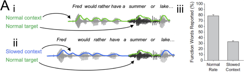
Figure 12.1A. Long description
Part A demonstrates the difference in speech waveforms between a normal speech rate context and a slowed speech rate context, both with the same target word, which reads," Fred would rather have a summer or a lake". A bar graph with an error bar in part A 3 compares the percentage of function words reported with the normal rate and slowed context. The mean percentage of function is 80% for the normal rate. The mean percentage of function is 35% for slowed context.
The SI hypothesis. (i) An illustration of SI for the normal context speech stimulus from (A). A mean speech rate (μ_1) is computed from the interpretation(s) of context speech. For each candidate interpretation of the target segment (“summer or” and “summer”), knowledge of each syllable’s relative duration is combined with μ_1 to obtain an estimated candidate duration. These estimated candidate durations are compared to the observed (e.g., acoustic) duration (ν). The candidate that best explains what is heard (in this case, the one most probable given the observed duration) is perceived. (ii) An illustration of SI for the slowed context speech stimulus from (A). Here, a slower mean speech rate (μ_2) leads to a different judgment of which candidate interpretation is most probable.
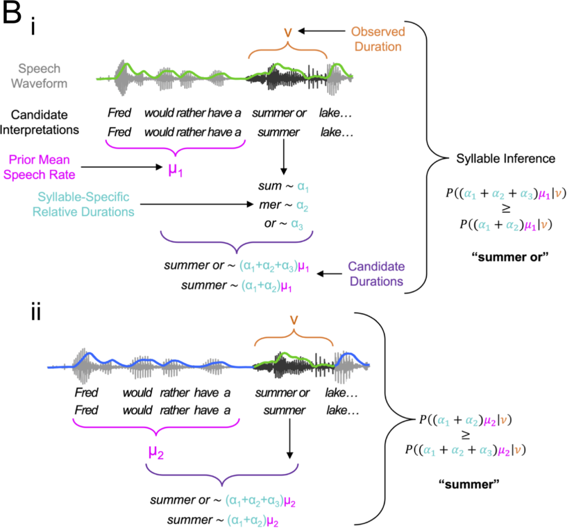
Figure 12.1B. Long description
Part B 1 illustrates a speech waveform along with the candidate's interpretations of the words that read: Fred would rather have a summer or a lake. A portion of words that read" Fred would rather have a" denotes my 1, which represents prior mean speech rate. An arrow from a sum points at a sum which is approximately equal to a 1, mer is approximately equal to a 2, which denotes syllable specific relative durations, or is approximately equal to a 3. The equations for candidate durations and syllable interference are given.
The unfolding of speech in time and the interdependence of speech content and timing imply that in the “guess-and-check” procedure of Bayesian inference, when guesses are made and how long it takes to make and check them are crucially important. Existing theoretical accounts have largely addressed the issue of timing in speech segmentation by leveraging syllabic-timescale brain rhythms as a dynamic and self-organizing mechanism of speech segmentation (Lakatos et al., Reference Lakatos, Shah and Knuth2005; Ghitza and Greenberg, Reference Ghitza and Greenberg2009; Shamir et al., Reference Shamir, Ghitza, Epstein and Kopell2009; Ghitza, Reference Ghitza2011, Reference Ghitza2013, Reference Ghitza2014, Reference Ghitza2020; Hyafil et al., Reference Hyafil, Fontolan, Kabdebon, Gutkin and Giraud2015; Hovsepyan et al., Reference Hovsepyan, Olasagasti and Giraud2020, Reference Hovsepyan, Olasagasti and Giraud2023; Friston et al., Reference Friston, Sajid and Quiroga-Martinez2021; Nabé et al., Reference Nabé, Schwartz and Diard2021; Su et al., Reference Su, MacGregor, Olasagasti and Giraud2023; Chapters 3 and 5). We pursue a different strategy: that of understanding the computational principles underlying word segmentation independently of their neurophysiological mechanisms (rhythmic or otherwise) (Doelling and Assaneo, Reference Doelling and Assaneo2021; Adolfi et al., Reference Adolfi, Wareham and van Rooij2023). Toward this end, we sketch how a recently proposed conceptual model of speech understanding – syllable inference (SI) (Figure 12.1B; Brown et al., Reference Brown, Tanenhaus and Dilley2021) – might be elaborated and extended within the Bayesian network formalism for probabilistic inference. SI builds on the frameworks of predictive coding (Millidge et al., Reference Millidge, Seth and Buckley2021), chunk-and-pass processing (Christiansen and Chater, Reference Christiansen and Chater2016), cue integration (Martin, Reference Martin2016), and analysis-by-synthesis (Halle and Stevens, Reference Halle and Stevens1962). It proposes that extracting meaning from spoken signals involves the dynamical generation of alternative candidate speech interpretations. Each candidate speech interpretation consists of a hierarchical model of morphosyntactic structure and a model of speech timing, linked at the syllabic timescale. These generate statistical predictions about the presence and timing of multiple acoustic cues that are compared to the speech signal. The interpretations that explain the speech input sufficiently well rise to the level of perception, leading to the phonemes, syllables, words, and phrases that listeners hear.
In the process of extending SI, we unpack the two timing-related chicken-and-egg problems confronted by the listener during word segmentation: the integration of holistic, context-dependent processing and time-bound, incremental processing; and the near-simultaneous inference of speech timing and speech content. In both cases, each process in the pair seems to depend on the prior completion of the other. We show how these problems are intimately related to narrowing the search space over speech interpretations without bias, and optimizing the speed/accuracy trade-off in language processing, employing concepts borrowed from machine learning and drift-diffusion-to-bound models of decision making. We make four claims about how listeners solve these problems: (1) Listeners model prosody and speech timing as part of a speaker model, as well as modeling morphosyntactic structure in a message model; (2) listeners incrementally infer the content and timing of “chunks” of speech comprised of variable-length sequences of morphosyntactic units, rather than individual morphosyntactic units; and (3) listeners adaptively schedule this irregular inference of content and timing, as well as the deployment of computationally intensive iterative search and optimization operations, using (4) predictable fluctuations in uncertainty accessible through the speaker model. We pull these four claims together in a mechanistic proposal – vowel-onset-paced syllable inference (VPSI) – and outline how VPSI accounts for repackaging effects, distal rate effects, and other aspects of speech psychophysics.
We begin with an interdisciplinary literature review. We first list the psychophysical properties of speech perception (including context dependence, incrementality, rate dependence, and repackaging and distal rate effects) that we propose any model of word segmentation must account for. We then situate the notion of a speaker model within the contexts of prosody, speech production, and linguistic communication more broadly. We briefly review Bayesian inference, generative modeling, and probabilistic approaches to speech processing, including the SI hypothesis. Finally, we explore computational aspects of online word segmentation and present the VPSI model.
12.2 Context and Timing in Speech Perception
12.2.1 Context Dependence in Speech Perception
Many psycholinguistic studies have shown the importance of context for speech perception and spoken word recognition. For example: speech sounds replaced by noise are perceptually “filled-in” (Warren, Reference Warren1970); phonemes and words pronounced intelligibly in longer utterances are unrecognizable when excised and presented alone (Pollack and Pickett, Reference Pollack and Pickett1963); and how a given phoneme is produced and perceived depends in a complex way on neighboring phonemes via coarticulation (e.g., the “sk-” in “ski” spliced with the “-ool” from “school” is perceived as “spool”) (Schatz, Reference Schatz1954). In terms of word segmentation and identification, the boundaries of phonological and morphosyntactic units (phonemes, syllables, words, etc.) are often – but not always – marked by acoustic cues (Heffner et al., Reference Heffner, Dilley, McAuley and Pitt2013). Thus, segmentation relies on the flexible, context-dependent integration (Mattys et al., Reference Mattys, White and Melhorn2005) of multiple cues across levels of analysis and timescales, including acoustic features (Stevens, Reference Stevens2002), phonotactics, allophones, coarticulation, syntax, semantics, and lexical competition (Mattys et al., Reference Mattys, White and Melhorn2005, Reference Mattys and Melhorn2007; Mattys and Melhorn, Reference Mattys and Melhorn2007), syllabic-level transitional probabilities (Morrill et al., Reference Morrill, Baese-Berk, Heffner and Dilley2015), and stress (Dilley et al., Reference Dilley and Pitt2010).
Theoretical perspectives in psycholinguistics have addressed two separable aspects of this context dependence: the context imposed by the hierarchical compositionality of linguistic structure itself; and the flexible use of varying sources of information to infer linguistic structure and meaning. The hierarchical structure of language – in which sentences are composed of sequences of words, which in turn are composed of sequences of syllables, which in turn are composed of sequences of phonemes – gives rise to interlocking constraints at multiple levels of abstraction (Christiansen and Chater, Reference Christiansen and Chater2016; Martin and Doumas, Reference Martin and Doumas2017; Martin, Reference Martin2020; Chapters 13 and 20). These provide stringent limits on the possible interpretations of speech signals.
Perhaps the broadest framework for understanding the flexible use of information in speech perception is cue integration (Martin, Reference Martin2016). In this framework, a cue is any signal or piece of information that reflects the linguistic structure and meaning of an utterance. This definition includes internally generated, linguistically abstract representations activated by knowledge and prior context (e.g., prior speech), for example syntactic structure as a cue to word class and discourse history as a cue to word identity and meaning. To infer speech interpretations, these cues are integrated in an approximately Bayesian way, weighted by their relative reliability. Cue integration construes language as the network of dependencies between different cues, with representations at each level of linguistic abstraction serving as cues to representations at other levels of abstraction. As we will see, this maps naturally onto the Bayesian network formalism.
12.2.2 Temporal Context in Speech: Incrementality and Rate Dependence
The specific temporal signatures of segmentation and lexical access are, themselves, highly context-dependent. The speed of word identification ranges from ∼200 ms after onset (within the first few phonemes) (Marslen-Wilson, Reference Marslen-Wilson1973; MacGregor et al., Reference MacGregor, Pulvermuller, Van Casteren and Shtyrov2012; Salverda et al., Reference Salverda, Kleinschmidt and Tanenhaus2014) in optimal conditions to considerably after onset in running speech (Bard et al., Reference Bard, Shillcock and Altmann1988). Distinct syllable and word structures can readily be inferred from subtle acoustic cues before, during (Pickett and Decker, Reference Pickett and Decker1960), or after (Miller and Liberman, Reference Miller and Liberman1979) a syllable boundary (see also Repp et al., Reference Repp, Liberman, Eccardt and Pesetsky1978; Galle et al., Reference Galle, Klein-Packard, Schreiber and McMurray2019), and acoustic information considerably after an acoustic event has elapsed can influence the speech content perceived (Miller and Liberman, Reference Miller and Liberman1979; Connine et al., Reference Connine, Blasko and Titone1993; Wade and Holt, Reference Wade and Holt2005).
Nevertheless, one important set of results demonstrates the rate dependence of speech processing. Speech is intelligible over a limited range of syllabic rates, with understanding of American English deteriorating quickly at syllabic rates above ∼9 Hz (two–three times the average rate of ∼3–5 Hz) (Beasley et al., Reference Beasley, Bratt and Rintelmann1980; Elliott and Theunissen, Reference Elliott and Theunissen2009; Ghitza and Greenberg, Reference Ghitza and Greenberg2009; Pefkou et al., Reference Pefkou, Arnal, Fontolan and Giraud2017). Experiments with repackaged speech suggest this limit is on the syllabic rate, and not the rate of segmental information (Ghitza and Greenberg, Reference Ghitza and Greenberg2009). Repackaging involves separating uniform chunks of compressed speech with uniform periods of silence, so that the segmental rate (controlled by the compression factor) and the syllabic rate (controlled by the silent interval length) are independent. Repackaging rescues intelligibility for speech compressed up to a factor of 6. The highest intelligibility occurs when a chunk of speech having an uncompressed duration of ∼333 ms (roughly, a syllable-sized chunk) is delivered at a rate below 9 Hz. This suggests a maximum “information rate” of ∼9 English syllables per second, regardless of the segmental rate (across languages, an information rate of ∼39 bits/s has been observed (Coupé et al., Reference Coupé, Oh, Dediu and Pellegrino2019). Within this limit, speech perception adjusts for the context speech rate, with, for example, the perception of ambiguous phonemes determined by the rate of adjacent phonemes, and sudden changes in speech rate altering the perception of subsequent vowel duration and word identity (Oganian et al., Reference Oganian, Kojima and Breska2023).
Experiments on temporal cues in speech understanding illuminate the potential mechanisms of this rate dependence. Modulations of the speech envelope, the profile of amplitude fluctuations ≤ 20 Hz in the speech waveform (Elliott and Theunissen, Reference Elliott and Theunissen2009; Edwards and Chang, Reference Edwards and Chang2013; Chapter 2), provide nearly all the information necessary to decipher speech (Shannon et al., Reference Shannon, Zeng, Kamath, Wygonski and Ekelid1995). Syllabic-timescale (∼1–9 Hz) fluctuations are predominant in these amplitude modulations (Elliott and Theunissen, Reference Elliott and Theunissen2009), and more generally, the integrity of information at syllabic timescales is uniquely critical for speech comprehension (Miller and Licklider, Reference Miller and Licklider1950; Huggins, Reference Huggins1964; Drullman et al., Reference Drullman, Festen and Plomp1994; Elliott and Theunissen, Reference Elliott and Theunissen2009). Neurophysiological explorations of speech comprehension have revealed that brain activity – including endogenous rhythmic activity at frequencies that mirror those of speech (e.g., phonemic, syllabic, and phrasal) (Lakatos et al., Reference Lakatos, Shah and Knuth2005) – tracks or synchronizes with the speech signal and with higher-order linguistic structure at multiple timescales (Ahissar et al., Reference Ahissar, Nagarajan and Ahissar2001; Luo and Poeppel, Reference Luo and Poeppel2007; Nourski et al., Reference Nourski, Reale and Oya2009; Hertrich et al., Reference Hertrich, Dietrich, Trouvain, Moos and Ackermann2012; Peelle et al., Reference Peelle, Gross and Davis2012; Doelling et al., Reference Doelling, Arnal, Ghitza and Poeppel2014; Di Liberto et al., Reference Di Liberto, O’Sullivan and Lalor2015; Ding et al., Reference Ding, Melloni, Zhang, Tian and Poeppel2016; Riecke et al., Reference Riecke, Formisano, Sorger, Başkent and Gaudrain2017; Keitel et al., Reference Keitel, Gross and Kayser2018; Zoefel et al., Reference Zoefel, Archer-Boyd and Davis2018; Oganian and Chang, Reference Oganian and Chang2019; Kojima et al., Reference Kojima, Oganian and Cai2021; Chapters 3, 5, 11, and 17). This speech–brain entrainment is associated with speech intelligibility (Ahissar et al., Reference Ahissar, Nagarajan and Ahissar2001; Luo and Poeppel, Reference Luo and Poeppel2007; Nourski et al., Reference Nourski, Reale and Oya2009; Hertrich et al., Reference Hertrich, Dietrich, Trouvain, Moos and Ackermann2012; Peelle et al., Reference Peelle, Gross and Davis2012; Doelling et al., Reference Doelling, Arnal, Ghitza and Poeppel2014; Ding et al., Reference Ding, Melloni, Zhang, Tian and Poeppel2016; Riecke et al., Reference Riecke, Formisano, Sorger, Başkent and Gaudrain2017; Zoefel et al., Reference Zoefel, Archer-Boyd and Davis2018; Chapters 3 and 5) and can even modulate speech understanding (Riecke et al., Reference Riecke, Formisano, Sorger, Başkent and Gaudrain2017; Wilsch et al., Reference Wilsch, Neuling, Obleser and Herrmann2018; Zoefel et al., Reference Zoefel, Archer-Boyd and Davis2018). Speech tracking depends in part on the brain’s response to spectro-temporal discontinuities or acoustic edges (Doelling et al., Reference Doelling, Arnal, Ghitza and Poeppel2014; Oganian and Chang, Reference Oganian and Chang2019; Kojima et al., Reference Kojima, Oganian and Cai2021; Chapters 3, 5, and 8), and neural activity is particularly sensitive to peak-rate events in the speech envelope, which are statistically associated with vowel onsets (Oganian and Chang, Reference Oganian and Chang2019) (in production, if not perception [Chapter 11]).
Going beyond this rate normalization and its mechanisms, distal rate effects (aka lexical rate effects) reveal that even the perceived number of morphosyntactic units in a given utterance can depend on context speech rate (Figure 12.1A; Dilley and Pitt, Reference Dilley and Pitt2010; Brown et al., Reference Brown, Dilley and Tanenhaus2012, Reference Brown, Tanenhaus and Dilley2021; Baese-Berk et al., Reference Baese-Berk, Heffner and Dilley2014; Pitt et al., Reference Pitt, Szostak and Dilley2016). In distal rate effects, subjects listen to and verbally repeat recorded sentences containing a target segment (“summer or”) with a reduced, coarticulated function word (“or”; Figure 12.1Ai). In some of these recordings, context speech is slowed while the target segment is left unaltered (Figure 12.1Aii). Subjects repeat back fewer function words for the slowed context (Figure 12.1Aiii). Sizeable effects of distal rate can occur even when word onsets are acoustically clear (Heffner et al., Reference Heffner, Dilley, McAuley and Pitt2013), and greater degrees of time expansion on distal context produce greater reductions in hearing a spoken word (Heffner et al., Reference Heffner, Dilley, McAuley and Pitt2013; Morrill et al., Reference Morrill, Dilley, McAuley and Pitt2013). Extensive explorations have found that distal rate effects occur only when rate-carrying context signals are intelligible, confirming that they cannot be accounted for by bottom-up, signal-driven processes alone (Pitt et al., Reference Pitt, Szostak and Dilley2016). Lexical rate effects are also manifestly probabilistic, depending in a graded way on the degree of alteration of context speech speed (Heffner et al., Reference Heffner, Dilley, McAuley and Pitt2013; Morrill et al., Reference Morrill, Dilley, McAuley and Pitt2013; Brown et al., Reference Brown, Tanenhaus and Dilley2021). Eye-tracking data from distal rate experiments show that determination of the presence of the ambiguous, blended word in the target segment was delayed until 800 ms after target segment offset (Brown et al., Reference Brown, Tanenhaus and Dilley2021), a delay considerably longer than other measurements of the timescale for uptake and use of segmental information (Salverda et al., Reference Salverda, Dahan and Tanenhaus2007; Lamekina and Meyer, Reference Lamekina and Meyer2023).
12.2.3 Context Dependence in Linguistic Communication
Accounts of linguistic communication increasingly have taken seriously the role of context in meaningful inference (Pickering and Garrod, Reference Pickering and Garrod2004; Stolk et al., Reference Stolk, Verhagen and Toni2016). Much of this work frames linguistic communication within the evolutionary imperative of social cognition (Hari et al., Reference Hari, Sams and Nummenmaa2016). This suggests an interdependence between inferences about intentions and meanings and inferences about speakers, speaker groups, and culturally specific linguistic variations (Macrae and Bodenhausen, Reference Macrae and Bodenhausen2001; Brown-Schmidt et al., Reference Brown-Schmidt, Yoon, Ryskin and Ross2015; Mattan et al., Reference Mattan, Kubota and Cloutier2017).
12.2.4 Timing in Speech Production
In the context of communication, the temporal dynamics of speech perception depend on those of speech production (Cutler et al., Reference Cutler, Dahan and Van Donselaar1997; Turk and Shattuck-Hufnagel, Reference Turk and Shattuck-Hufnagel2014; Brown-Schmidt et al., Reference Brown-Schmidt, Yoon, Ryskin and Ross2015; McQueen and Dilley, Reference McQueen, Dilley, Gussenhhoven and Chen2020; Chapters 2, 6, and 7). Apart from the morphosyntactic structure of speech, a major determinant of speech timing is prosody, a hierarchical linguistic structure that defines the groupings and intonations of words, as well as the stress and prominence of words and syllables (Cutler et al., Reference Cutler, Dahan and Van Donselaar1997; Turk and Shattuck-Hufnagel, Reference Turk and Shattuck-Hufnagel2014; Chapters 17 and 18). Prosodic structure may be indicated acoustically by the pitch, timing, and duration of words and syllables relative to each other, as in phrase-final lengthening. However, no acoustic cue is diagnostic of prosodic structure, which language users impute even in the absence of relevant acoustic cues, and, indeed, while reading (Cutler et al., Reference Cutler, Dahan and Van Donselaar1997; Breen et al., Reference Breen, Fitzroy and Oraa Ali2019; McQueen and Dilley, Reference McQueen, Dilley, Gussenhhoven and Chen2020).
Speech timing is also influenced by factors not considered prosodic, including speech speed – of central importance in our account – as well as speech style, pragmatics, discourse-level semantics, emotion, clarity requirements, movement costs, and cognitive, motor, and physiological constraints (Turk and Shattuck-Hufnagel, Reference Turk and Shattuck-Hufnagel2014; Watson et al., Reference Watson, Jacobs and Buxó-Lugo2020; Chapters 1, 2, 6, 7, 15, 16, and 18). For example, word duration, often a marker of stress, is also influenced by word predictability, by speakers’ level of engagement, and by production difficulty (Watson et al., Reference Watson, Jacobs and Buxó-Lugo2020). Similarly, the placement of phrase boundaries – often considered to reflect prosodic and syntactic considerations – can reflect cognitive capacity, as suggested by evidence correlating interindividual variability in prosodic phrase length with working memory capacity (which presumably limits speakers’ planning scope) (Bishop and Intlekofer, Reference Bishop and Intlekofer2020).
Thus, prosody and other extra-morphosyntactic factors shape speech timing and acoustics to reflect not only the speaker’s intended message but also the speech production process, and the computational, cognitive, and physiological constraints and contexts under which speech production is occurring. In turn, this information reflects and provides clues to the emotional and physiological state, cognitive capacity, intentions, and identity of the speaker, providing a wealth of information relevant to a speaker model.
12.3 Probabilistic and Generative Modeling in Speech Perception
12.3.1 Speech Perception as Generative Modeling and Probabilistic Inference
Generative (i.e., top-down, synthetic, or predictive) modeling and probabilistic inference have a long history in linguistic theory. In the early analysis-by-synthesis framework for speech recognition (Halle and Stevens, Reference Halle and Stevens1962; Bever and Poeppel, Reference Bever and Poeppel2010), well-learned, bottom-up filters extract a rough interpretation; an internal generative model constructs a set of alternative interpretations accounting for longer-timescale contextual dependencies and predicts their sensory consequences; and the best predictor of the input is the final interpretation.
Bayesian statistical models provide a principled, quantitative approach to integrating knowledge- and signal-based cues (Martin, Reference Martin2016; Norris et al., Reference Norris, McQueen and Cutler2016), and have been applied to word segmentation (Norris and McQueen, Reference Norris and McQueen2008; Hovsepyan et al., Reference Hovsepyan, Olasagasti and Giraud2020, Reference Hovsepyan, Olasagasti and Giraud2023; Friston et al., Reference Friston, Sajid and Quiroga-Martinez2021; Nabé et al., Reference Nabé, Schwartz and Diard2021; Su et al., Reference Su, MacGregor, Olasagasti and Giraud2023), syntactic parsing (Traxler, Reference Traxler2014), and language learning (Abend et al., Reference Abend, Kwiatkowski, Smith, Goldwater and Steedman2017) and evolution (Griffiths and Kalish, Reference Griffiths and Kalish2007; Moulin-Frier et al., Reference Moulin-Frier, Diard, Schwartz and Bessière2015). Bayes’ theorem describes how prior beliefs should be combined with current observations during inference, expressing the conditional probability of an event A given an observation B, P(A|B), as (a multiple of) the product of the prior probability of the event, P(A), and the likelihood of the observation given the event, P(B|A). The distribution P(B|A) can be interpreted as a generative model of the data, which is inverted when calculating the posterior probability P(A|B).
Recent applications of Bayesian inference to cognition and neurophysiology broadly (Rao and Ballard, Reference Rao and Ballard1999; Knill and Pouget, Reference Knill and Pouget2004; Friston et al., Reference Friston, Kilner and Harrison2006, Reference Friston, Daunizeau and Kiebel2009; Adams et al., Reference Adams, Shipp and Friston2013; Millidge et al., Reference Millidge, Seth and Buckley2021) emphasize the brain’s function as a “prediction engine” that maintains an internal (generative) model of the world and continually produces hypotheses about the most likely causes of sensory data. This generative model biases inference toward conclusions that are probable given prior experience and current knowledge, but also enables rapid, accurate inference in the face of considerable variability and uncertainty. Updating the model to eliminate prediction errors (mismatches between predictions and observations) leads to both perception and learning, with uncertainty (or its inverse, precision) determining the relative adjustment of hypotheses and data. Predictive coding is a simple algorithmic implementation of this process (Rao and Ballard, Reference Rao and Ballard1999; Millidge et al., Reference Millidge, Seth and Buckley2021). A generative model can be formalized as a set of (probability distributions over) hypothetical causal factors known as hidden or latent variables that probabilistically determine observed variables or states (i.e., sensory data). Precision is not directly observable and must be predicted by second-order hidden variables (Koelsch et al., Reference Koelsch, Vuust and Friston2019), which are updated through confirmation or disconfirmation of first-order predictions. The brain is believed to implement a deep (i.e., multi-level) hierarchical generative model, in which hidden and observed variables are arranged into a compositional hierarchy like that observed in language (Friston et al., Reference Friston, Trujillo-Barreto and Daunizeau2008). The relationships between hidden and observed variables in a generative model can be captured in a Bayesian network.Footnote 1
12.3.2 Rhythm-Mediated Segmentation in Probabilistic Models
Leveraging experimental results on speech–brain entrainment, influential hypotheses have suggested that speech segmentation and sampling are mediated by a speech-entrained hierarchy of neural oscillators (Ghitza and Greenberg, Reference Ghitza and Greenberg2009; Ghitza, Reference Ghitza2011; Giraud and Poeppel, Reference Giraud and Poeppel2012). In one prominent set of proposals, a θ-frequency (∼4–8 Hz) oscillator tracks syllabic-timescale fluctuations in the speech amplitude envelope, driving a γ (∼40–60 Hz) oscillator that samples phonemic information at a rate proportional to the syllabic rate (Ghitza, Reference Ghitza2011; Giraud and Poeppel, Reference Giraud and Poeppel2012; Chapter 9). In this and similar accounts, the self-organized, history-dependent dynamics of brain rhythms are imputed to integrate prior speech speed with speech acoustics to perform accurate segmentation. Indeed, a recent model suggests that a neurophysiologically inspired oscillator exhibiting frequency and phase adaptation can implement something like Bayesian inference of event duration (Doelling et al., Reference Doelling, Arnal and Assaneo2023).
Several recent computational models integrate rhythmic accounts of syllable segmentation with probabilistic generative modeling of morphosyntactic structure (Hovsepyan et al., Reference Hovsepyan, Olasagasti and Giraud2020, Reference Hovsepyan, Olasagasti and Giraud2023; Friston et al., Reference Friston, Sajid and Quiroga-Martinez2021; Nabé et al., Reference Nabé, Schwartz and Diard2021; Su et al., Reference Su, MacGregor, Olasagasti and Giraud2023). These models fit under the umbrella of the Bayesian network formalism, with several models employing an approximate inference scheme that relies on free-energy minimization.Footnote 2 They employ oscillators or oscillator-inspired mechanisms to implement segmentation at the level of syllables, which in turn enables word- or lemma-level inference (Hovsepyan et al., Reference Hovsepyan, Olasagasti and Giraud2020, Reference Hovsepyan, Olasagasti and Giraud2023; Nabé et al., Reference Nabé, Schwartz and Diard2021; Su et al., Reference Su, MacGregor, Olasagasti and Giraud2023). While all make invaluable and pioneering contributions, none of them performs online word segmentation of naturalistic speech: one segments speech post hoc rather than online (Friston et al., Reference Friston, Sajid and Quiroga-Martinez2021); some have been implemented only on small synthetic “languages” whose units have regular duration (Nabé et al., Reference Nabé, Schwartz and Diard2021; Su et al., Reference Su, MacGregor, Olasagasti and Giraud2023); and some recognize syllables but not words (Hovsepyan et al., Reference Hovsepyan, Olasagasti and Giraud2020, Reference Hovsepyan, Olasagasti and Giraud2023). More importantly, the rhythm-inspired mechanisms used to determine speech timing and syllable onsets in most models do not receive feedback from the probabilistic models inferring morphosyntactic structure (Hovsepyan et al., Reference Hovsepyan, Olasagasti and Giraud2020, Reference Hovsepyan, Olasagasti and Giraud2023; Nabé et al., Reference Nabé, Schwartz and Diard2021; Su et al., Reference Su, MacGregor, Olasagasti and Giraud2023). While these mechanisms exhibit their own bottom-up adaptation to fluctuations in the temporal structure of speech acoustics, they cannot integrate information about content – for example, the number of words imputed to a given speech segment. The SI hypothesis takes a step toward rectifying this omission by outlining the bidirectional interactions between inference of timing and content.
12.3.3 The Syllable Inference Hypothesis
As discussed in Section 12.1, SI proposes that extracting meaning from spoken signals involves the dynamical generation of alternative candidate speech interpretations, each consisting of a hierarchical model of morphosyntactic structure and speech timing and prosody, including speed, stress, and phrasal contours, with a key focus on the syllable (Figure 12.1B; Brown et al., Reference Brown, Tanenhaus and Dilley2021). From this ensemble of models, those that explain the speech input sufficiently well (minimizing prediction error, maximizing model evidence, and/or surpassing some minimum level of confidence) rise to the level of perception, leading to the phonemes, syllables, words, and phrases that listeners hear. Under SI, each interpretation generates statistical predictions about the presence and timing of multiple time-frequency cues in the input. These predictions or hypotheses are based on the morphosyntactic and prosodic hierarchies imputed by the interpretation, estimates of the current speech rate and rhythm, and language-specific knowledge about the relative duration and timing of segments, syllables, words, and phrases. The arrival or absence of the cues predicted by any interpretation triggers a re-evaluation of the goodness-of-fit of the ensemble of current candidate interpretations, and potentially the updating of that ensemble to include new candidates.
Acoustic edges are a broad class of such cues (Stevens, Reference Stevens2002; Doelling et al., Reference Doelling, Arnal, Ghitza and Poeppel2014; Oganian and Chang, Reference Oganian and Chang2019; Kojima et al., Reference Kojima, Oganian and Cai2021; Chapter 8), and SI predicts that they provide evidence (in the form of prediction errors) for the processes of model evaluation and generation. Recognizing that the syllabic timescale is privileged both in speech acoustics and the neural dynamics of speech perception, SI asserts that the detection of syllabic-timescale temporal landmarks in particular – a highly reliable source of evidence pertaining to both the phonetic and the prosodic structure of speech – triggers neural activity implementing the evaluation and generation of candidate speech interpretations. SI postulates that the most reliable acoustic evidence of a syllable boundary occurs following that boundary, at the onset of the vocalic nucleus of the next syllable, an acoustic event to which the brain is exquisitely sensitive (Oganian and Chang, Reference Oganian and Chang2019). This indicates that all pertinent information regarding the previous syllable has arrived, and thus that interpretation of that syllable can be completed.
At the same time, rhythmic processes driven by reliable (acoustic or linguistic) evidence of syllable boundaries perform the dual functions of tracking speech speed and evaluating the relative timing of speech input. Rhythmic syllabic-timescale population activity thus encodes a probability distribution over speech speed, inferred from the timing of previous (perceived) syllables. As speech unfolds, the evolving estimate of the mean speech rate affects both the suite of candidate speech interpretations and the predicted relative timing of sound units. Deviations from predicted durations must be explained by positing alternative hypotheses as to the sources of variation (e.g., local lengthening for emphasis), or by updating the estimated speech rate. According to SI, the neural activity implementing these calculations – hypothesis generation and evaluation and inference of speech speed and rhythm – is what results in the statistical phase-locking of neural oscillations to the speech amplitude envelope, and the association of speech intelligibility with speech–brain entrainment at syllabic timescales.
12.4 Computational Challenges in Online Word Segmentation
As the SI hypothesis draws on the framework of predictive processing, Bayesian networks provide a natural framework for its computational construction. Here, we sketch this construction in a way intentionally agnostic to neurophysiological implementations, while assuming such implementations exist and making use of empirical observations about the relative timing of brain activity and speech. We take this approach to clarify the computational challenges inherent in online word segmentation (Table 12.1), and to allow these challenges and their solutions to constrain and guide the search for neurophysiological mechanisms, rather than the other way around. Along the way, we aim to reconcile incremental processing with the (temporally extended) hierarchical representation of sequences of linguistic units, to explain repackaging effects and distal rate effects in speech perception, and to provide an explanation of just how speech content and speech speed are estimated concurrently.
A non-comprehensive attempt to connect computational challenges to strategies for their solution and potential mechanisms of implementation. Note that challenges, solution strategies, and possible mechanisms are highly overlapping.
| Computational challenge | Solution strategies | Possible mechanisms |
|---|---|---|
| Accuracy | Using all available evidence | Post hoc inference |
| Long-timescale evidence accumulation | High-level latent variables in deep hierarchical models | |
| Inferring sequences of morphosyntactic units | ||
| Synthetic mechanisms | ||
| Speed | Using evidence as it becomes available | Continuous inference (i.e., filtering) |
| Short-timescale evidence consolidation | Incremental (i.e., Markov) assumption | |
| Balancing speed and accuracy, i.e., | Employing a priori constraints | Bayesian inference |
| Integrating holistic and incremental inference, i.e., | Inferring causal variables at multiple levels of abstraction | Deep hierarchical generative modeling |
| Managing search space size | Posing hypotheses at optimal level of abstraction | |
| Alternating filtering with synthetic mechanisms | Periodic post hoc re-estimation | |
| Adaptively alternating filtering and synthetic mechanisms | Pacing post hoc re-estimation by observed and/or predicted precision | |
| Alternating between evidence accumulation and evidence consolidation | Periodic model updates and/or fluctuations in precision | |
| Adaptively switching between evidence accumulation and evidence consolidation | Pacing model updates by observed and/or predicted precision | |
| Urgency-like signals based on estimated information rate | ||
| Inferring both timing and content | Alternating timing and content inference (i.e., expectation maximization) | Periodically alternating model updates and/or fluctuations in precision |
| Periodic post hoc re-estimation | ||
| Adaptively switching between timing and content inference | Pacing model updates by observed and/or predicted precision | |
| Urgency-like signals based on estimated information rate | ||
| Pacing post hoc re-estimation by observed and/or predicted precision | ||
| Minimizing the impact of computationally intensive operations | Adaptively switching between evidence accumulation and evidence consolidation | Pacing model updates by observed and/or predicted precision |
| Urgency-like signals based on estimated information rate | ||
| Adaptively scheduling iterative and synthetic operations | Pacing post hoc re-estimation by observed and/or predicted precision |
12.4.1 Generative Models Predict Speech Timing and Content
First, we specify a generative model, consisting of a hierarchy of dynamic (i.e., time-dependent) probability distributions. As in existing work, this generative model encodes the morphosyntactic structure of the message through probability distributions over the word, syllable, and phoneme levels of linguistic organization (Figure 12.2A; Nabé et al., Reference Nabé, Schwartz and Diard2021). To account for distal rate effects, we must at least keep track of (i.e., infer) speech rate alongside morphosyntactic structure; SI proposes that word segmentation also makes use of the duration of individual syllables relative to the speech rate (Brown et al., Reference Brown, Tanenhaus and Dilley2021). Thus, we specify a hierarchical generative model of speech timing, with variables representing the mean syllabic rate and individual syllable and phoneme durations (Figure 12.2A). Together, these two conditionally independent hierarchies specify the acoustics of the speech signal. A model of speech timing, as part of a speaker model (Brown-Schmidt et al., Reference Brown-Schmidt, Yoon, Ryskin and Ross2015) potentially governed by the temporal regularities of speech production (Elliott and Theunissen, Reference Elliott and Theunissen2009; Bishop and Intlekofer, Reference Bishop and Intlekofer2020; Ten Oever and Martin, Reference Ten Oever and Martin2021), begins to address the communicative context of speech (Brown-Schmidt et al., Reference Brown-Schmidt, Yoon, Ryskin and Ross2015).
Distal rate effects and the SI hypothesis.
A hierarchical Bayesian network for word segmentation. Hierarchically organized latent variables representing sequences of words (Wordi), syllables (Syli), and phonemes (Φi) constitute a generative model of morphosyntactic structure. Hierarchically organized latent variables representing syllabic rate (Rate) and sequences of syllable durations (DSyl,i) and phoneme durations (DΦ,i) constitute a generative model of speech timing. Together, they specify a speech signal as a trajectory in feature space.
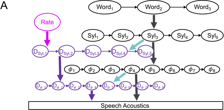
Figure 12.2A. Long description
Part A: A hierarchical structure of words, syllables, and their corresponding acoustic features, represented by D. The arrows indicate the flow of information from higher-level units to lower-level units and, ultimately, to the Speech Acoustics features. The sign phi represents transformations or mappings between levels.
Interdependence of contextual and incremental processing. The size of each increment depends on the mean rate, and vice versa. Left and right show two different interdependent sets of increments and mean rate.
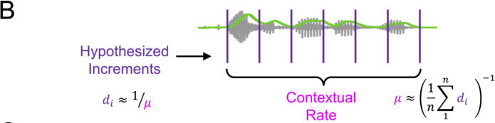
Figure 12.2B. Long description
Part B: A waveform with four vertical lines drawn over it is labeled contextual rate. The hypothesized increments representing the wave reads, d i, are approximately equal to 1 over mu. An equation on the right side reads, mu is approximately one, open large bracket, one over n sigma 1 to n d i, close large bracket raised to the power of minus 1.
The VPSI mechanism. A rate prior enables rate-dependent inference of content. When reliable timing information arrives, it triggers post hoc content re-estimation, which leads to rate re-estimation and a rate posterior. This serves as the rate prior for rate-dependent content inference of the next chunk of speech.

12.4.2 Sequences Not Units Are Inferred
Distal rate effects demonstrate that only a sequence of units reliably contains enough contextual information to disambiguate the speech signal. Thus, in SI, candidate speech interpretations may contain different numbers of words, syllables, and phonemes. We propose that this must be operationalized by defining hidden variables (at all levels in both hierarchies) as single distributions over sequences of units, rather than sequences of distributions over individual units (Figure 12.2A).
Inferring sequences accords not only with the highly context-dependent nature of speech but also with the essentially fungible nature of the division of speech into units on evidence in processes of language learning and evolution (Christiansen and Chater, Reference Christiansen and Chater2016). Further, it aligns with a framing in which the ultimate goal of linguistic communication is guiding adaptive action in support of survival and reproductive success (Chapters 6, 7, 15, 16, 18, and 29). We propose that this goal takes priority over the decoding of linguistic content, and can be achieved in its absence, for example by deciphering the emotion and intent of a speaker of a foreign language (Frühholz and Schweinberger, Reference Frühholz and Schweinberger2021). We suggest that meaning making, similarly, can occur without the identification and segmentation of specific linguistic units by mapping stretches of speech to sequences of linguistic units of any length – for example, through the holistic identification of commonly used multi-word expressions.
12.4.3 Inference Proceeds Incrementally
Next, we specify an inference algorithm to invert the generative model. Given a speech signal, this scheme should output a probability distribution over possible sequences of words and syllabic rates, which can be used (along with some utility function) to select a single most likely or appropriate interpretation. Exact inference involves enumerating the set of possible sequences of words and syllabic rates; calculating the likelihood of the speech input given each sequence, and multiplying it by the prior probability of the sequence; and then normalizing to find the distribution over possible sequences.
This approach maximizes the accuracy of inference by using all the information contained in an utterance to determine its probable interpretations. However, it is slow, and not only because it requires waiting until the end of the utterance. While a longer speech signal offers more evidence to distinguish between interpretations, it also has a larger number of possible interpretations. Indeed, large search spaces make exact inference impossible in practice for most problems. Generally speaking, both exhaustive search processes and their reformulations as iterative computations – including, for example, prediction error minimization (Tschantz et al., Reference Tschantz, Millidge, Seth and Buckley2023) – have costs in terms of time and resources that scale with search space size, and efficiency requires avoiding, minimizing, or carefully timing them (Halle and Stevens, Reference Halle and Stevens1962; Tschantz et al., Reference Tschantz, Millidge, Seth and Buckley2023). This trade-off between the information content of the evidence and the size of the search space – that is, between the speed and the accuracy of inference – can also be viewed as a tension between context dependence and incrementality in processing. This tension is particularly easy to understand in the case of speech rate inference (Figure 12.2B). Here, the context (mean speech rate) informs incremental inference (via estimated syllable duration), and must simultaneously be derived from multiple incremental estimates (Figure 12.2B).
Thus, even presented with an entire utterance at once – for example, during reading – the most efficient strategy employs one “piece” of evidence at a time, incrementally constraining the space of possible interpretations. In online inference, time offers a natural way to parcel out evidence, and all existing models of online speech inference make a temporal incremental approximation. That is, they approximate the distribution over word sequences and speech speeds that best explains the entire utterance with a series of distributions over word sub-sequences and speech speeds, each of which best explains the input up to a given time. This is accomplished in practice by iteratively updating the posterior distribution, adjusting it based on the inversion of the generative model for one “chunk” of input at a time; we assume that the sequence of words best explaining the first and second chunks of input is reasonably approximated by the sequence of words A that best explains the first chunk of input, followed by the sequence of words B that, given A, best explains the second chunk of input.
Formally, we assume a Markov property at each hierarchical level of the model. This means the distribution over sequences of morphosyntactic units (e.g., phonemes) explaining the current chunk of speech is independent of all but the previous chunk, given the current distribution over sequences of higher-level units (e.g., syllables). Why is lower-level units’ independence from the past conditional on higher-level units? Because the structure of speech is compositional in time, distributions over higher-level units effectively encode (some aspects of) an arbitrarily long past context, as well as their influence on sequences of lower-level units. Thus, deep hierarchical representations allow arbitrarily long past context to influence inference at all levels, even if the distant past is not explicitly represented at lower levels (Friston et al., Reference Friston, Trujillo-Barreto and Daunizeau2008; Martin and Doumas, Reference Martin and Doumas2017; Martin, Reference Martin2020). This makes it possible to assume a Markov property (i.e., independence from the past) without losing long-timescale contextual information. This point illustrates that deep hierarchical modeling is roughly equivalent to the modeling of distant temporal context. By modeling, for example, sequences at the word level, we roughly approximate the modeling of deeper hierarchical levels of linguistic structure such as syntax and meaning; and by modeling sequences of speech speeds, we could potentially approximate the modeling of higher levels of prosodic structure.
This temporal compression is just one manifestation of the information compression inherent in the compositional structure of hierarchical generative models. In general, this structure lowers search costs without sacrificing accuracy, by enabling alternatives to be enumerated at high hierarchical levels with small search spaces and evaluated at low hierarchical levels with high information density. Thus, a hierarchical morphosyntactic model enables us to account for the current stretch of speech by searching for possible word (rather than syllable or phoneme) sequences, while determining the likelihood of those sequences from acoustic features (rather than inferred phonemes or syllables).
12.4.4 Evidence Accumulation Alternates with Model Updating across Processing Streams
If inference is to be incremental, it remains to specify the size of the increments – that is, what constitutes a chunk. Given that speech inputs of a fixed duration will invariably represent (and be interpreted as) sequences of morphosyntactic units of variable length – and more basically, because the number and duration of morphosyntactic units is exactly what we hope to infer during word segmentation – we propose that the length of a chunk cannot be specified in terms of a fixed number of morphosyntactic units, at any level of analysis. It is tempting to define the length of a chunk relative to the speed of speech; but how are we to obtain a reliable estimate of the speech speed without first inferring speech content? A variation on the issues discussed in the previous section, this question highlights two new issues: the importance of establishing informative prior probabilities over speech content and speed; and the difficulty of simultaneously inferring the “what” and the “when” of speech (Figure 12.2B).
Regarding the first, we propose that speech patterns facilitate estimates of speech speed and content at the beginning of an utterance – for example with highly stressed and/or predictable monosyllabic utterances such as greetings or interjections (Norrick, Reference Norrick2009). We can illustrate the latter obstacle in a simple template-matching account of speech perception. Ignoring variation in the pronunciation of individual morphosyntactic units, we think of each linguistic unit as a noisy trajectory through some feature space, and the listener as possessing linguistic knowledge comprised of “canonical” or “prototypical” trajectories for each unit (e.g., word, syllable, or phoneme). The computational goal is to determine what sequence of units comprise the speech signal; an auxiliary goal is to determine the speed at which these units are replayed. If we knew the sequence of units, it would be trivial to determine the speed by stretching the corresponding sequence of canonical trajectories to match, as well as possible, the observed trajectory. If all trajectories were traversed at the same known speed, we could recover the sequence of units – even unit by unit – by finding the sequence of canonical trajectories that best match the observed trajectory. In the case where we know neither the speed nor the content, the space of possible trajectories includes all possible sequences, of all possible lengths, replayed at all possible speeds. Notably, the transition from one unit to the next can occur at any time. In fact, some automatic speech recognition algorithms (and TRACE, the early interactive activation model of word segmentation [McClelland and Elman, Reference McClelland and Elman1986]) find unit onset times by comparing unit templates having all possible onsets to the data.
The central issue here is that when we must infer two mutually dependent variables (e.g., timing and content), the search space grows very fast with the data length. One well-known method for the efficient simultaneous inference of two mutually dependent variables is expectation maximization (EM) (Dempster et al., Reference Dempster, Laird and Rubin1977). EM involves repeatedly inferring one variable while holding the other constant, using updated expectations about one variable to improve inference of the other, until the likelihood of the combined guess arrives at a (locally) maximal value. From the perspective of a single variable, past inferences about the other variable are evidence to be integrated in the current inference process.
In Precoss-β, a recent model integrating probabilistic and rhythmic mechanisms to infer the identities and durations of syllables from naturalistic speech (Hovsepyan et al., Reference Hovsepyan, Olasagasti and Giraud2023), such an alternation was implemented via rhythmic fluctuations in prediction error precision (PEP). PEP determines how prediction errors are weighted in model updates. When PEP is high, models are adjusted to eliminate prediction errors, and as a result prediction errors have low magnitude; when PEP is low, models follow their own internal dynamics, and large prediction errors are “allowed” to remain. Notably, a model exhibiting rhythmic fluctuations in PEP identified syllables more effectively than one in which PEP was held constant, because periods of low PEP effectively served as windows for evidence accumulation, while subsequent periods of high PEP consolidated the accumulated evidence into a single model update. Interestingly, this alternation was most advantageous at β frequency, and was most effective when the PEP for syllable boundaries and syllable identities fluctuated in antiphase, resulting in alternating estimation of “when” a syllable occurred and “what” syllable occurred (Hovsepyan et al., Reference Hovsepyan, Olasagasti and Giraud2023). There is evidence that β rhythms are related to fluctuations in precision in multiple brain systems: In the visual cortex, rhythms in sensitivity of visual target detection (Fiebelkorn et al., Reference Fiebelkorn, Saalmann and Kastner2013) also involve β oscillations (Fiebelkorn et al., Reference Fiebelkorn, Pinsk and Kastner2018) that have been interpreted as representing predictions of precision (Aussel et al., Reference Aussel, Fiebelkorn, Kastner, Kopell and Pittman-Polletta2023); and in a model of the basal ganglia, β rhythms have been implicated in the maintenance of the currently active motor plan (Chartove et al., Reference Chartove, McCarthy, Pittman-Polletta and Kopell2020), which in active inference is a function of precision (Adams et al., Reference Adams, Shipp and Friston2013).
Coming full circle, inference over hierarchical generative models effectively implements an alternation between contextual and incremental processing. High-level distributions represent context informing low-level incremental inference; and low-level increments then inform updates to high-level contextual representations. This alternation is straightforward to implement when increments are regular and fixed, as in a recent model inferring sentential context from speech waveforms for a small set of examples containing syllables, lemmas, and sentences with uniform or contextually determined durations (Su et al., Reference Su, MacGregor, Olasagasti and Giraud2023).
12.4.5 Predicted Precision Paces Incremental Inference
Suggestively, the syllabic-timescale structure of speech is already favorably arranged for an alternating inference procedure, via the (statistical) alternation between vocalic nuclei and consonantal clusters (Nespor et al., Reference Nespor, Pena and Mehler2003; Ghitza, Reference Ghitza2013; Sun and Poeppel, Reference Sun and Poeppel2023). Vocalic nuclei, as we’ve discussed, are prominent features of speech acoustics (Chapters 5 and 11). Because vowels are smaller in number and longer in duration than consonants in most languages, vocalic nuclei potentially afford the inference of the time (window) of occurrence of a single linguistic unit with high precision, providing an important temporal landmark for speech perception that informs language learning early in development (Hochmann et al., Reference Hochmann, Benavides-Varela, Nespor and Mehler2011). Consonantal clusters, meanwhile, are composed of multiple temporally fleeting acoustic cues that can in aggregate provide highly reliable evidence about phoneme sequence identity, offering an opportunity to anchor the inference of speech content (Sun and Poeppel, Reference Sun and Poeppel2023; Chapter 39) relied on by adult listeners (Hochmann et al., Reference Hochmann, Benavides-Varela, Nespor and Mehler2011). Interestingly, the power of the β rhythms associated with visual sampling and motor plan maintenance are nested within ongoing θ rhythms (i.e., their power fluctuates at θ frequency) (Chartove et al., Reference Chartove, McCarthy, Pittman-Polletta and Kopell2020; Aussel et al., Reference Aussel, Fiebelkorn, Kastner, Kopell and Pittman-Polletta2023).
However, in Precoss-β, syllabic (i.e., θ) timescale alternations in PEP were less effective than β frequency alternations (Hovsepyan et al., Reference Hovsepyan, Olasagasti and Giraud2023). We propose that this is because, at the syllabic timescale, the effectiveness of alternating between inference of “what” and “when” is dependent on the alignment of the “what” phase with consonantal clusters, and the “when” phase with vocalic nuclei. Generally speaking, the issue here is that the information content of speech is not uniformly distributed in time; nor does it need to be for accurate speech perception, as demonstrated by, for example, repackaging. This suggests that, while rhythms may offer a hard-coded heuristic for the alternation of precision between different variables during online inference, the most effective way to alter precision is based on informed predictions or estimates of its fluctuation over the course of the speech signal.
The principles at play here are illuminated by results from drift-diffusion-to-bound models of decision making, in which evidence is integrated across time until a decision threshold is reached (Ratcliff et al., Reference Ratcliff, Smith, Brown and McKoon2016). This decision threshold varies across tasks and decisions, and even during single decisions, with the duration of deliberation (Malhotra et al., Reference Malhotra, Leslie, Ludwig and Bogacz2018). This variation depends on neural activity encoding both the conditional probability of obtaining further information (e.g., the hazard rate of occurrence of some probabilistic event [Herbst et al., Reference Herbst, Fiedler and Obleser2018]) and the opportunity cost of deliberation (i.e., how much potential reward is lost by continuing to deliberate), dubbed the urgency (Cisek et al., Reference Cisek, Puskas and El-Murr2009; Thura et al., Reference Thura, Cos, Trung and Cisek2014). Urgency alters the decision threshold or the speed of evidence accumulation, tuning the speed–accuracy trade-off to obtain the greatest possible cumulative reward (Cisek et al., Reference Cisek, Puskas and El-Murr2009; Thura et al., Reference Thura, Cos, Trung and Cisek2014). For example, relatively speaking, a task with a high reward rate will engender a high level of urgency and a low decision threshold, because a high error rate is less costly, in terms of cumulative reward, than a slow rate of return.
A similar trade-off is inherent in timing the shift from evidence gathering or accumulation to evidence integration or consolidation. Here, the quantity to be maximized is cumulative information gain rather than cumulative reward. One strategy for navigating this trade-off is to delay evidence integration until there is either a high level of precision or reliability, or a clear “decision point” or “deadline” (Hawkins et al., Reference Hawkins, Wagenmakers, Ratcliff and Brown2015). We propose that chunking (i.e., evidence integration) occurs when precision either meets or is predicted to meet a particular threshold. At the level of syllables, vowel onsets serve as both a highly reliable temporal landmark and a deadline for evidence integration (Ghitza, Reference Ghitza2013, Reference Ghitza2020), and may be predicted by a model of speech timing and prosody. Similarly, a sufficiently precise estimate of speech rate may provide an endogenous deadline for evidence integration. Interestingly, perceived speech speed reflects cognitive load (Bosker et al., Reference Bosker, Reinisch and Sjerps2017); we suggest that increased cognitive load decreases the level of certainty attainable in the time available to make a decision about speech content – that is, it requires lowering a decision threshold – which is interpreted subjectively as an increase in speech speed.
This notion of adaptive chunking furnishes an account of repackaging effects in which the silent interval between (signal-based) chunks provides a predictable cue for evidence consolidation. This account predicts that a different such cue – such as a tone, or a repeated nonsense syllable – would have the same effect as a silent interval. In language games such as Geta or Gibberish and Op, the easy intelligibility of speech in which a nonsense string such as “itig” or “op” is inserted at the beginning (between the onset and rime) of each syllable (Kazanina et al., Reference Kazanina, Bowers and Idsardi2018) provides anecdotal support for this hypothesis.
Adaptive chunking may also pace the timing of costly iterative inference. Reliable temporal landmarks such as vocalic nuclei and silent gaps in speech may be leveraged to engage synthetic mechanisms as in analysis-by-synthesis, or the backward pass of Bayesian smoothing. These periods of evidence integration over longer timescales may increase the certainty of inference and allow for reassessment of the interpretations of past data given new information. Furthermore, the timing of computations by estimates of precision may serve to align the cognitive, neural, and physiological processes of listeners to those of speakers (Pickering and Garrod, Reference Pickering and Garrod2004; Chapter 29) in the service of creating a shared conceptual and experiential space (Stolk et al., Reference Stolk, Verhagen and Toni2016). This may allow speech timing to cue content inference prospectively (Ten Oever and Martin, Reference Ten Oever and Martin2021) as well as retrospectively, as when a pause that’s longer than usual prompts the recovery of a double, less common, or more subtle meaning for previous words or phrases.
12.5 Vowel-Onset-Paced Syllable Inference
We integrate these ideas in a model called vowel-onset-paced syllable inference (VPSI). To illustrate VPSI, we return to the simplified template-matching account of segmentation described above (Section 12.4.4), in which we think of speech as a trajectory in feature space. The dimensions of this space represent phonemic features including, for example, vocalic or consonantal identity, position and manner of articulation (for consonants), openness and frontness (for vowels), nasalization, syllabification, and so on (see Moulin-Frier and Arbib, Reference Moulin-Frier and Arbib2013, for an example). We add a dimension representing the rate of change of the broadband speech amplitude envelope. We also assume two independent sources of noise – one contaminating the instantaneous rate of the envelope and another contaminating the phonemic dimensions of feature space.
12.5.1 VPSI Combines Rate-Dependent Content Inference with Irregular Re-estimation of Content and Rate
In VPSI, each candidate speech interpretation consists of a word sequence, which determines probability densities over syllable and phoneme sequences and over trajectories in feature space. (A phoneme sequence is mapped to a trajectory in feature space by concatenating canonical trajectories for individual phonemes.) Evidence for a given word sequence is calculated as the likelihood of the speech input given this probability distribution on trajectories in feature space, and accumulates continuously. VPSI begins with content inference informed by expectations about rate: The onset of an utterance initiates a filtering process of evidence accumulation about speech content, with the speed of rollout of candidate interpretations determined by the rate expected according to a prior on speech speed (i.e., by the expectation of this prior; Figure 12.2C). Independent evidence of vowel onsets is determined by the rate of change of the broadband speech envelope. Note that because VPSI infers a distribution over sequences of units, transitions between units are probabilistic events. The probability of a transition at a given point in time is determined by both the sum of probabilities over the set of sequences making a transition at that time and the rate of change of the broadband amplitude envelope.
In line with our proposal that inference is adaptively paced, and that speech speed depends on speech content, updates of the speech rate distribution occur at temporal landmarks (Figure 12.2C). These landmarks occur when either of two conditions is met: the level of precisionFootnote 3 of the distribution over speech content passes a threshold; or the probability of a transition passes a threshold. The latter can occur if the probability distribution over phoneme, syllable, or word sequences is such that nearly all probable sequences exhibit a transition at the same time point. It can also occur when a peak-rate event in the broadband speech amplitude envelope signals a vowel onset.
When a temporal landmark occurs, it triggers a post hoc re-estimation of both the timing and the content of the speech elapsed since the previous landmark (or since the onset of speech, if the current landmark is the first; Figure 12.2C). This involves using the transitional chunk of speech between landmarks to calculate evidence for a new set of candidate interpretations, each of which is associated with a different speech rate. These are determined by (e.g., sampled from) the current priors on speech rate and over word sequences, (i.e., the posteriors on speech rate and word sequences calculated at the previous and current temporal landmarks, respectively). For a given candidate interpretation, the likelihood of the transitional chunk factors as a product of the likelihood of the observed content (i.e., the trajectory in phonemic feature space) and the likelihood of the observed duration sequence (determined, to first order, by a linear scaling of the template for that interpretation). After re-estimation, the durations associated with the best-fitting template are used to update the speech rate distribution (Figure 12.2C). Thus, estimates of speech speed rely not only on the intervals between vowel onsets but also on the imputed distributions over syllable sequences for each chunk of speech.
12.5.2 VPSI Accounts for Results on Repackaging and Distal Rate Effects
Without vowel onsets, the response of VPSI depends on the signal-to-noise ratio (SNR) for phonemic features, and how close the speech rate is to the speech rate prior. If phonemic features are clear, and the speech rate prior is close to the actual speech rate, then content inference will reach a high level of precision. When this high precision triggers re-estimation, it ensures the set of candidate interpretations considered will have low morphosyntactic variance, varying mostly in speech rate. We propose this will result in rapid re-estimation that mostly serves to update speech rate based on the most-probable morphosyntactic candidate structures. If phonemic features are unclear, or the speech rate prior is not close to the actual speech rate, content inference will be imprecise, and there will be no updates of speech rate, resulting in a global failure to reach precision in inference.
If vowel onsets (or other reliable cues to speech timing) are present, even with inter-onset intervals corresponding to frequencies in the tails of the speech speed prior, we claim that the performance of VPSI will depend on the SNR for phonemic features alone. This is because even for a high phonemic feature SNR, a speech rate prior that is far off the mark will lead to a low level of certainty about speech content. Thus, the re-estimation of speech content will be primarily prompted by vowel onsets. This re-estimation will involve a large suite of candidate interpretations, whose speech rates are drawn from the tails of the current rate prior, enabling the sequential adjustment of the speech rate distribution. Note that despite large variability in the speech rate, the number of syllables these candidates contain is quantized, because the syllabic “distance” between two vowel onsets must be a whole number (e.g., it must consist of one, two, or three syllables), significantly reducing re-estimation’s computational cost. Another advantage of re-estimating at salient vowel onsets is that the computationally intensive re-estimation process occurs during the vocalic nucleus, a period of time when the information rate of speech is relatively low (Sun and Poeppel, Reference Sun and Poeppel2023).
We suggest this situation provides an account of repackaging effects, with the silent gaps inserted between packages playing the role of reliable timing cues. This interpretation suggests two factors contributing to the ∼9 Hz ceiling on the syllabic rate. The second is the support of the speech rate prior, that is, the interval over which most of the prior’s probability mass is distributed; this may be speaker-, listener-, and language-specific. For instance, in English, the number of possible syllables between vowel onsets is three, and the ceiling is three times the mean syllabic rate; we predict that in moraic languages such as Japanese, the ceiling on the syllabic rate will be a lower multiple of the average speech rate. Likely even more important is the duration of the re-estimation process; this process, which we propose normally occurs following vowel onset, is triggered in this case by the onset of the silent period, and must fit within the silent interval.
In distal rate effects, vowel onsets occur in the first syllable of the target segment and following the target segment, but not during the reduced function word. Despite a high phonemic feature SNR, the ambiguity of the coarticulated, blended target content results in imprecise content inference. Thus, when the vowel onset following the target segment triggers re-estimation, both the with (function word) and without (function word) interpretations will be within the re-estimation search space. The content of both interpretations has a high likelihood, and we assume they are equally likely given prior speech. Thus, the competition between the two interpretations will be decided by the likelihood of their respective imputed duration sequences, and with certain assumptions it should be possible to write down the probability of choosing one interpretation over another.Footnote 4
12.6 Conclusion
We suggest that in online speech inference, strict temporal constraints advantage computational efficiency, above and beyond tractability or computability (Adolfi et al., Reference Adolfi, Wareham and van Rooij2023). Like others (Halle and Stevens, Reference Halle and Stevens1962; Christiansen and Chater, Reference Christiansen and Chater2016; Martin and Doumas, Reference Martin and Doumas2017; Brown et al., Reference Brown, Tanenhaus and Dilley2021; Friston et al., Reference Friston, Sajid and Quiroga-Martinez2021; Hovsepyan et al., Reference Hovsepyan, Olasagasti and Giraud2023), we highlight the cost of search operations (Tschantz et al., Reference Tschantz, Millidge, Seth and Buckley2023), the size of the search space, and the speed–accuracy trade-off as major computational challenges.
We propose that listeners address these challenges with adaptive timing of inference. EM-like inferential turn taking between processing streams (e.g., “what” and “when”) (Dempster et al., Reference Dempster, Laird and Rubin1977; Hovsepyan et al., Reference Hovsepyan, Olasagasti and Giraud2023) and hierarchical levels (at timescales characteristic of each level [Halle and Stevens, Reference Halle and Stevens1962; Friston et al., Reference Friston, Trujillo-Barreto and Daunizeau2008; Christiansen and Chater, Reference Christiansen and Chater2016; Martin and Doumas, Reference Martin and Doumas2017; Su et al., Reference Su, MacGregor, Olasagasti and Giraud2023]) optimize the timing of evidence accumulation and evidence consolidation. These alternations are timed by second-order predictions of temporal fluctuations in precision (e.g., the syllabic-timescale alternation between temporally informative vowels and phonologically informative consonants [Nespor et al., Reference Nespor, Pena and Mehler2003; Ghitza, Reference Ghitza2013; Sun and Poeppel, Reference Sun and Poeppel2023]), located within a generative model of speech timing that heavily overlaps with a speaker model predicting temporal regularities arising from physiological, motor, and cognitive processes (Elliott and Theunissen, Reference Elliott and Theunissen2009; Bishop and Intlekofer, Reference Bishop and Intlekofer2020; Ten Oever and Martin, Reference Ten Oever and Martin2021). Listeners may use such temporal information to pace their own computational, neural, and even neurophysiological processes, aligning them with those of the speaker (Pickering and Garrod, Reference Pickering and Garrod2004; Chapter 29). This “cooperative pacing” may facilitate the construction of a shared conceptual space (Stolk et al., Reference Stolk, Verhagen and Toni2016) and allow listeners to leverage aspects of speech production that facilitate information transfer (Aylett and Turk, Reference Aylett and Turk2004; Mahowald et al., Reference Mahowald, Dautriche, Gibson and Piantadosi2018; Ten Oever and Martin, Reference Ten Oever and Martin2021).
Incorporating a hierarchical generative model of speech timing, the VPSI model performs rate-based continuous inference of speech content, re-estimating the rate and content of recent speech using generative, synthetic mechanisms when sufficient precision about speech content or timing is attained. Content precision triggers rapid re-estimation; timing precision triggers computationally intensive re-estimation occurring when the content information rate is low. Re-estimation in VPSI accounts for both repackaging and distal rate effects, iteratively improving speech rate estimates and resolving ambiguity in speech content.
We predict timing-related prediction errors, and processes of model evaluation and construction following reliable temporal cues, should have neurophysiological traces. The neural signatures of precision should alternate between brain regions computing and representing distinct processing streams and hierarchical levels. If speech rate estimates depend on both lexical and acoustic cues, then lexical manipulations can affect rate perception, as well as vice versa; distal rate effects may require the content precision provided by syntactic and semantic structure (Pitt et al., Reference Pitt, Szostak and Dilley2016); and data requirements for rate estimation may underlie results on minimum intelligible segments excised from running speech (Pollack and Pickett, Reference Pollack and Pickett1963).
Expressing the computational problem of online segmentation mathematically (Adolfi et al., Reference Adolfi, Wareham and van Rooij2023) is crucial to precisely articulating and quantifying the impact of the challenges discussed. So is clarifying whether the adaptive updating mechanisms illustrated in VPSI are “built in” to predictive processing via free-energy minimization in hierarchical generative models, or must be explicitly engineered in (Hovsepyan et al., Reference Hovsepyan, Olasagasti and Giraud2023; Tschantz et al., Reference Tschantz, Millidge, Seth and Buckley2023). A deeper understanding of the computational and algorithmic architecture of word segmentation (Adolfi et al., Reference Adolfi, Wareham and van Rooij2023) can provide a platform for exploring the neural signatures (and potential implementations) of speech perception (Doelling and Assaneo, Reference Doelling and Assaneo2021), through biophysically detailed brain region- and operation-specific neurophysiological mechanisms and mathematical models (Oganian and Chang, Reference Oganian and Chang2019; Cannon, Reference Cannon2021; Cannon and Patel, Reference Cannon and Patel2021; Doelling and Assaneo, Reference Doelling and Assaneo2021; Frühholz and Schweinberger, Reference Frühholz and Schweinberger2021; Pittman-Polletta et al., Reference Pittman-Polletta, Wang and Stanley2021; Doelling et al., Reference Doelling, Arnal and Assaneo2023; Gwilliams et al., Reference Gwilliams, King, Marantz and Poeppel2022; Adolfi et al., Reference Adolfi, Wareham and van Rooij2023).
12.7 Acknowledgements
We thank Jon Cannon, Sevada Hovsepyan, Yohan John, Tom Lagatta, Mamady Nabé, Itsaso Olasagasti, Johanna Rimmele, Yaqing Su, and an anonymous reviewer for many useful discussions and comments that contributed to this work.
Summary
We propose that the probabilistic modeling of speech timing plays a key role in word segmentation, by predicting the reliability of speech information across channels and linguistic levels. These predictions enable the efficient and adaptive timing of model updates and resource-intensive computations, supporting an optimal trade-off between speed and accuracy.
Implications
This proposal implies that extra-morphosyntactic regularities predict fluctuations in the uncertainty of the speech signal, and that cognitively demanding operations occur during times of low predicted uncertainty. It suggests experiments assessing the relationship between higher-order speech statistics, behavior, and neural activity that distinguish the proposed mechanisms from influential bottom-up accounts.
Gains
Our account of prosodic modeling for speech understanding formulates detailed, novel hypotheses about how the brain times information processing across modalities and the linguistic hierarchy. These have the potential to advance both the understanding of human speech processing and its neurophysiology, and the performance of artificial language systems.
13.1 Speech Processing as Information Transmission through Constrained Channels
Speech is crucial in our daily lives, enabling direct interaction and communication. Understanding speech is a complex process due to its transient and intricately structured nature. Indeed, speech sounds can be abstracted at multiple levels of analysis, speech being a multiplexed signal displaying levels of complexity, organizational principles, and perceptual units of analysis at distinct timescales.
How does the brain build the diverse representational linguistic units at different timescales from the speech signal? This process is even harder given the fleeting nature of speech and human memory limitation. Indeed, speech comprehension faces the “now or never bottleneck” (Christiansen and Chater, Reference Christiansen and Chater2016). This means that if listeners do not process relevant information in a fast and incremental fashion, they may lose the opportunity to understand it altogether. Therefore, the speed at which information (being acoustic or linguistic in nature) is conveyed in speech – the information rate – is a more relevant dimensional space than the absolute amount of information conveyed (information value) to the brain (Coupé et al., Reference Coupé, Oh, Dediu and Pellegrino2019). This is because our neurocognitive resources are limited and can only process a certain amount of information in a given amount of time, leading to temporal bottlenecks (Hasson et al., Reference Hasson, Yang, Vallines, Heeger and Rubin2008; Honey et al., Reference Honey, Thesen and Donner2012; Lerner et al., Reference Lerner, Honey, Silbert and Hasson2011; Vagharchakian et al., Reference Vagharchakian, Dehaene-Lambertz, Pallier and Dehaene2012). By understanding these bottlenecks and their implications, we can better understand how we process speech.
A potential way of uncovering general principles of speech perception is to describe and determine the temporal constraints that shape its processing at each level of speech analysis. As such, in this chapter, we will show that a meticulous characterization of the various levels of organization found in speech and language, their temporal constraints and their relation to comprehension, can provide valuable and novel insights into an individual’s speech processing ability.
Speech processing in the human brain can be conceptualized as a process of information integration through channels with limited capacities. The auditory system continuously receives a complex stream of sound waves that needs to be processed and decoded in real time into meaningful information to understand the messages conveyed by the speaker. This process involves several stages of analysis, from low-level acoustic processing to high-level semantic interpretation (Christiansen and Chater, Reference Christiansen and Chater2016; Hickok and Poeppel, Reference Hickok and Poeppel2007; Rosen, Reference Rosen1992). One of the key challenges of speech processing is dealing with the limited capacity of our neural resources, which results from intrinsic biological constraints. This implies that speech signals or speaking situations that do not conform with these constraints result in poor comprehension.
Building on previous work (Coupé et al., Reference Coupé, Oh, Dediu and Pellegrino2019; Ghitza, Reference Ghitza2013; Gibson et al., Reference Gibson, Futrell and Piantadosi2019; Pellegrino et al., Reference Pellegrino, Coupé and Marsico2011; Reed and Durlach, Reference Reed and Durlach1998), we recently proposed to determine how the limited capacity of our neural resources and the complexity of linguistic features in speech constrain our ability to comprehend spoken language (Giroud et al., Reference Giroud, Lerousseau, Pellegrino and Morillon2023). We proposed to rely on a concept inherited from information theory (Shannon, Reference Shannon1948), channel capacity. Within this framework, each level of the speech processing hierarchy can be modeled as a transfer of information through a dedicated channel. Channel capacity is defined as the maximum amount of information that can be transmitted through this communication channel without errors or loss, in bits per second (bits/s). It can be also referred to as a temporal (processing) bottleneck, in which information is processed at a fixed speed (Vagharchakian et al., Reference Vagharchakian, Dehaene-Lambertz, Pallier and Dehaene2012). Hence, if too much information arrives per unit of time, information transfer is suboptimal or fails. Using such a normative measurement framework allowed for the determination of multilevel linguistic processing constraints limiting speech comprehension. This suggests that speech perception is hierarchical (Millert et al., Reference Millert, Caucheteux and Orhan2022), with sequential bottlenecks, each with its own channel capacity. Hereafter, we will provide an account of diverse experimental works that brought insights about the relevant processing bottlenecks involved in speech comprehension. We will focus on work spanning multiple levels of analysis from acoustic to higher-level linguistic features to determine their respective channel capacity. More precisely, we hereafter characterize the following linguistic features: the speech acoustic timescales; the syllabic timescale; the phonemic timescale; higher-level linguistic timescales such as words, phrases, and sentences; and lexical information rates and contextual information, as derived from deep neural networks (Figure 13.1; see also Giroud et al., Reference Giroud, Lerousseau, Pellegrino and Morillon2023).
Speech characterization at multiple levels of analysis.
Rate (in Hz) or information rate (in bits/s) of seven linguistic features of an example sentence. Features are described from low to high linguistic levels: acoustic temporal modulation rate (in Hz), syllabic rate (in Hz), phonemic rate (in Hz), syllabic information rate (in bit/s), phonemic information rate (in bit/s), static lexical surprise (i.e., word frequency) (in bit/s), and contextual lexical surprise (in bit/s).

13.2 The Speech Acoustic Timescales
First and foremost, speech is a complex acoustic signal that involves variations in frequency and intensity over time. These low-level acoustic features can be described in terms of spectro-temporal modulations (Elliott and Theunissen, Reference Elliott and Theunissen2009), and are critical for the intelligibility of speech. On one hand, the spectral (or frequency) dimension is a crucial aspect of the speech signal. It corresponds to the distribution of the energy of the sound signal in the frequency scale (sound spectrum), and makes it possible to define the different formants of the speech units (in particular, the vowels) and their transitions (Stevens and Klatt, Reference Stevens and Klatt1974). On the other hand, the temporal dimension of the speech sounds is highly relevant for comprehension (Albouy et al., Reference Albouy, Benjamin, Morillon and Zatorre2020; Shannon et al., Reference Shannon, Zeng, Kamath, Wygonski and Ekelid1995; Smith et al., Reference Smith, Delgutte and Oxenham2002). This second dimension indexes the precise organization of the different elements of speech over time.
When producing speech, the dynamics of the vocal tract articulators are translated in a waveform that displays fluctuations in signal amplitude over time. This pattern is referred to as the speech signal’s envelope, and its main temporal modulation is typically situated between 2 and 8 Hz, with an average maximum around 4–5 Hz (Ding et al., Reference Ding, Patel and Chen2017; Varnet et al., Reference Varnet, Ortiz-Barajas, Erra, Gervain and Lorenzi2017). Critically, this characteristic range is preserved across speakers, languages, and speaking conditions (Ding et al., Reference Ding, Patel and Chen2017; Poeppel and Assaneo, Reference Poeppel and Assaneo2020). Speech thus appears to be temporally structured, a feature that the brain might capitalize on to further process relevant information. Multiple temporal modulations are crucial for comprehension, including those within the 1–7 Hz range related to phrases, words, and syllables (Elliott and Theunissen, Reference Elliott and Theunissen2009; Meyer, Reference Meyer2018). Temporal modulations above 12 Hz are linked to specific phonetic features and segmental information (Chapter 9; Christiansen et al., Reference Christiansen, Greenberg and Henrichsen2009; Drullman et al., Reference Drullman, Festen and Plomp1994; Rosen, Reference Rosen1992; Shannon et al., Reference Shannon, Zeng, Kamath, Wygonski and Ekelid1995). Speech signals lacking the naturally occurring envelope temporal modulations are less intelligible (Chi et al., Reference Chi, Gao, Guyton, Ru and Shamma1999, Reference Chi, Ru and Shamma2005; Elhilali et al., Reference Elhilali, Chi and Shamma2003; Elliott and Theunissen, Reference Elliott and Theunissen2009). Moreover, removing the main temporal fluctuations (2–9 Hz) within spoken stimuli by artificially filtering the signal results in degraded intelligibility for listeners. And artificially restoring these temporal modulations – by the addition of brief noise bursts that act as temporal cues at exactly where the “acoustic edges” of the original stimuli were – leads to a drastic increase in intelligibility (Doelling et al., Reference Doelling, Arnal, Ghitza and Poeppel2014; Ghitza, Reference Ghitza2012).
13.3 Neural Tracking of the Speech Acoustic Dynamics
At the neural level, the auditory cortex effectively represents the speech envelope (Nourski et al., Reference Nourski, Reale and Oya2009; Shamma, Reference Shamma2001). Theta band (4–8 Hz) neural activity consistently aligns with the speech envelope, which closely approximates the syllabic timescale (Chapter 3; Giraud and Poeppel, Reference Giraud and Poeppel2012; Luo and Poeppel, Reference Hickok and Poeppel2007). However, theta activity primarily encodes acoustic rather than linguistic features (Etard and Reichenbach, Reference Etard and Reichenbach2019). Although crucial for intelligibility, the speech envelope indeed only indirectly reflects syllabic rate, which is rather landmarked by acoustic onset edges (Oganian and Chang, Reference Oganian and Chang2019; Schmidt et al., Reference Schmidt, Chen and Keitel2023; Zhang et al., Reference Zhang, Zou and Ding2023). Neural tracking of the speech envelope is hence a necessary, but not sufficient, condition for comprehension (Ahissar et al., Reference Ahissar, Nagarajan and Ahissar2001; Brodbeck and Simon, Reference Brodbeck and Simon2020; Kösem et al., Reference Kösem, Dai, McQueen and Hagoort2023). Additionally, while natural speech’s temporal modulation rate is around 5 Hz, neural processes can adapt to acoustic rates up to 15 Hz, beyond which comprehension is hindered (Giroud et al., Reference Giroud, Lerousseau, Pellegrino and Morillon2023). This channel capacity associated with the acoustic modulation rate has a strong impact on speech comprehension, and is independent from syllabic or any other linguistic features. Taken together, the above results converge to reveal the central role of the temporal envelope in speech processing.
13.4 The Syllabic Timescale
The hierarchical structure of language implies the existence of different linguistic units that are combined in different ways to create an infinite number of meanings. While currently there is no consensus on the nature of the fundamental unit of speech recognition, it is generally accepted that features described in phonetics are at work during language perception. Two pre-lexical levels of description have been subject to intense neurophysiological investigation due to their relevance for speech perception: phoneme-sized units (either of a phonetic or a phonemic nature) and syllable-sized units (Giraud and Poeppel, Reference Giraud and Poeppel2012; Mesgarani et al., Reference Mesgarani, Cheung, Johnson and Chang2014; Poeppel and Assaneo, Reference Poeppel and Assaneo2020).
Syllables last between 150 and 300 ms, with an average around 200 ms (Ghitza and Greenberg, Reference Ghitza and Greenberg2009; Greenberg, Reference Greenberg2001; Rosen, Reference Rosen1992). This corresponds to a rate of 2.5–8 syllables per second in natural settings (Coupé et al., Reference Coupé, Oh, Dediu and Pellegrino2019; Kendall, Reference Kendall2013; Pellegrino et al., Reference Pellegrino, Coupé and Marsico2011; Zhang et al., Reference Zhang, Zou and Ding2023). The syllable is an essential unit of all languages, with regard to acquisition, pathologies, language errors, and psycholinguistic processing (Dolata et al., Reference Dolata, Davis and Macneilage2008).
Accordingly, the syllabic timescale is the strongest linguistic determinant of speech comprehension (Giroud et al., Reference Giroud, Lerousseau, Pellegrino and Morillon2023). Previous research using speeded speech has provided evidence that beyond 15 syllables per second, speech becomes unintelligible (Dupoux and Green, Reference Dupoux and Green1997; Foulke and Sticht, Reference Foulke and Sticht1969; Ghitza, Reference Ghitza2014; Giroud et al., Reference Giroud, Lerousseau, Pellegrino and Morillon2023; Nourski et al., Reference Nourski, Reale and Oya2009); 15 Hz would hence be the channel capacity associated with syllabic processing (Giroud et al., Reference Giroud, Lerousseau, Pellegrino and Morillon2023). Further use of time-compressed spoken materials showed that compressing natural speech three times or more impairs comprehension but that this effect is strongly alleviated by the insertion of periods of silence between time-compressed speech segments (Ghitza and Greenberg, Reference Ghitza and Greenberg2009). In particular, restoring the “syllabicity” of the spoken stimuli (its original temporal structure in terms of the syllable rate) seems to be the optimal way to partially restore comprehension of highly compressed speech. Overall, this suggests that the online tracking of individual syllables is a strong prerequisite for speech comprehension.
13.5 The Phonemic Timescale
While the syllabic timescale and its neural underpinning has been investigated in depth, the contribution and neural substrate of the phonemic timescale to speech comprehension is less clear. Phonemes are the smallest linguistic units of speech sounds and represent a generalization or abstraction over different phonetic realizations. Phonemes are the smallest perceptual unit capable of determining the meaning of a word (e.g., beer and peer differ only with respect to their initial phonemes). They last typically between 60 and 150 ms in natural speech, with the majority being around 50–80 ms (Ghitza and Greenberg, Reference Ghitza and Greenberg2009; Rosen, Reference Rosen1992). This corresponds to a rate of approximately 10–15 phonemes per second in natural speech (Studdert-Kennedy, Reference Studdert-Kennedy, Smelser and Gerstein1986). Phonemes are associated with a processing bottleneck whose channel capacity is of ~35 Hz (Giroud et al., Reference Giroud, Lerousseau, Pellegrino and Morillon2023). However, the phonemic rate has only a residual impact on speech comprehension (Giroud et al., Reference Giroud, Lerousseau, Pellegrino and Morillon2023), which suggests that the online tracking of individual phonemes is not a prerequisite for speech comprehension. Instead, acoustic phonetic representations of speech are encoded during natural speech perception (Mesgarani et al., Reference Mesgarani, Cheung, Johnson and Chang2014; Nourski et al., Reference Nourski, Steinschneider and Rhone2015), with multiple speech sounds being encoded in parallel at any given time, together with their relative order within the speech sequence (Gwilliams et al., Reference Gwilliams, King, Marantz and Poeppel2022).
Phonemes are, however, a relevant unit of representation for speech processing. During their first months, infants have the ability to discriminate most phonemic contrasts present in multiple languages (Gervain, Reference Gervain2015; Mahmoudzadeh et al., Reference Mahmoudzadeh, Dehaene-Lambertz and Fournier2013; Moon et al., Reference Moon, Lagercrantz and Kuhl2013), and about six months after birth, this ability becomes more focused on native phonemes (Kuhl, Reference Kuhl2000; Kuhl et al., Reference Kuhl, Ramírez, Bosseler, Lin and Imada2014). Interestingly, this specialization in processing native phonemes is linked to an increase in synchronization of low-gamma band (~25–50 Hz) neural activity (Ortiz-Mantilla et al., Reference Ortiz-Mantilla, Hämäläinen, Realpe-Bonilla and Benasich2016; see Menn et al., Reference Menn, Männel and Meyer2023, for a perspective). In adults, neural dynamics in the low-gamma band are also observed during auditory processing (Lakatos et al., Reference Lakatos, Shah and Knuth2005; Lehongre et al., Reference Lehongre, Ramus, Villiermet, Schwartz and Giraud2011; Morillon et al., Reference Morillon, Lehongre and Frackowiak2010, Reference Morillon, Liégeois-Chauvel, Arnal, Bénar and Giraud2012) and notably track the amplitude envelope of speech (Di Liberto et al., Reference Di Liberto, O’Sullivan and Lalor2015; Fontolan et al., Reference Fontolan, Morillon, Liegeois-Chauvel and Giraud2014; Gross et al., Reference Gross, Hoogenboom and Thut2013; Lehongre et al., Reference Lehongre, Ramus, Villiermet, Schwartz and Giraud2011; Lizarazu et al., Reference Lizarazu, Lallier and Molinaro2019). Whether this phenomenon reflects phonemic-categorical processing or lower-level acoustic or phonetic processing remains unclear. Work by Marchesotti et al. (Reference Marchesotti, Nicolle and Merlet2020) provides evidence of the crucial role played by low-gamma band neural dynamics in processing phonemic information during speech perception. In their study, they recorded electroencephalography (EEG) data from dyslexic participants and found that activity at 30 Hz was lower than that of neurotypical adults. They then used transcranial alternating current stimulation (tACS) to temporarily restore low-gamma neural dynamics in dyslexic adults. Interestingly, this intervention led to improved phonological processing and reading performance, but only when the stimulation was targeted at 30 Hz (versus 60 Hz) and in the group of participants with dyslexia. These findings support a connection between low-gamma neural oscillations and phonological processing.
13.6 Higher-Level Linguistic Timescales
Phonemes and syllables are combined to form larger units such as words, phrases, and sentences. The length, variability, and rhythmicity of these higher-level linguistic structures have been investigated (Breen, Reference Breen2018; Clifton et al., Reference Clifton, Carlson and Frazier2006). These (post-)lexical timescales, however, are of the same order of magnitude as prosodic dynamics, making their specific investigation difficult (but see Section 3). In particular, in spoken languages, prosodic information (intonation, pauses) naturally fluctuates around 0.5–3 Hz, which encompasses phrasal and word-level timescales (Auer et al., Reference Auer, Couper-Kuhlen and Muller1999; Ghitza, Reference Ghitza2017; Inbar et al., Reference Inbar, Grossman and Landau2020; Stehwien and Meyer, Reference Stehwien and Meyer2022). Such speech dynamics are tracked by neural dynamics in the same range, which corresponds to the delta frequency band (Bonhage et al., Reference Bonhage, Meyer, Gruber, Friederici and Mueller2017; Boucher et al., Reference Boucher, Gilbert and Jemel2019; Bourguignon et al., Reference Bourguignon, De Tiège and de Beeck2013; Buiatti et al., Reference Buiatti, Peña and Dehaene-Lambertz2009; Gross et al., Reference Gross, Hoogenboom and Thut2013; Meyer et al., Reference Meyer, Henry, Gaston, Schmuck and Friederici2017; Molinaro et al., Reference Molinaro, Lizarazu, Lallier, Bourguignon and Carreiras2016; Park et al., Reference Park, Ince, Schyns, Thut and Gross2015). The distinctive role of these delta rate dynamics in the temporal cortex for prosodic tracking and high-level linguistic processes has been documented (Bourguignon et al., Reference Bourguignon, De Tiège and de Beeck2013; Ding et al., Reference Ding, Melloni, Zhang, Tian and Poeppel2016; Keitel et al., Reference Keitel, Gross and Kayser2018; Kösem and van Wassenhove, Reference Kösem and van Wassenhove2017; Lamekina and Meyer, Reference Lamekina and Meyer2023; Lu et al., Reference Lu, Jin, Ding and Tian2023; Molinaro and Lizarazu, Reference Molinaro and Lizarazu2018; Rimmele et al., Reference Rimmele, Sun, Michalareas, Ghitza and Poeppel2023; Vander Ghinst et al., Reference Vander Ghinst, Bourguignon and Op de Beeck2016), but their respective channel capacity remains to be explored. Of note, this phrasal tracking occurs even in the absence of distinct acoustic modulations at the phrasal rate (Ding et al., Reference Ding, Melloni, Zhang, Tian and Poeppel2016; Kaufeld et al., Reference Kaufeld, Bosker and Ten Oever2020; Keitel et al., Reference Keitel, Gross and Kayser2018). However, diverging evidence led to the proposal to dissociate delta neural activity driven by acoustically driven segmentation following prosodic phrases from activity that indexes knowledge-based segmentation of semantic/syntactic phrases (Lu et al., Reference Lu, Jin, Ding and Tian2023; Meyer, Reference Meyer2018). Currently, the role of delta neural dynamics in speech processing is still vigorously debated (Boucher et al., Reference Boucher, Gilbert and Jemel2019; Giraud, Reference Giraud2020; Inbar et al., Reference Inbar, Grossman and Landau2020; Kazanina and Tavano, Reference Kazanina and Tavano2023; Lo et al., Reference Lo, Henke, Martorell and Meyer2023).
Strikingly, during speech perception, spontaneous finger tapping at the perceived (prosodic) rhythm of speech occurs within the delta range (i.e., at ~2.5 Hz; see Lidji et al., Reference Lidji, Palmer, Peretz and Morningstar2011). A similar effect is visible during music perception, with spontaneous movements occurring at the perceived beat, around 0.5–4 Hz (Merchant et al., Reference Merchant, Grahn, Trainor, Rohrmeier and Fitch2015; Morillon et al., Reference Morillon, Arnal, Schroeder and Keitel2019; Rajendran et al., Reference Rajendran, Teki and Schnupp2018). These findings point toward a preference of attentional and motor systems for the slow (~0.5–3 Hz) temporal dynamics of auditory streams. Accordingly, during speech processing, delta oscillations are not only visible in temporal areas but also in the motor cortex (Giordano et al., Reference Giordano, Ince and Gross2017). And delta motor cortical dynamics uniquely contribute to both the modulation of auditory processing and comprehension: On the one hand, the tracking of acoustic dynamics by the (left) auditory cortex is principally modulated by motor areas, through delta (and to a lesser extent theta) oscillatory activity (Keitel et al., Reference Keitel, Ince, Gross and Kayser2017; Park et al., Reference Park, Ince, Schyns, Thut and Gross2015). On the other hand, in motor areas, both delta tracking of the phrasal acoustic rate and delta-beta coupling predict speech comprehension (Keitel et al., Reference Keitel, Gross and Kayser2018).
13.7 From Speech Rate to Information Rate
Past works have characterized the properties of language in terms of informational content exchange and transmission using large cross-linguistic corpora and the information theory framework (Shannon, Reference Shannon1948). In this context, “information” does not refer to message meaning but to its unpredictability or unexpectedness (Coupé et al., Reference Coupé, Oh, Dediu and Pellegrino2019; Oh et al., Reference Oh, Coupé, Marsico and Pellegrino2015; Pellegrino et al., Reference Pellegrino, Coupé and Marsico2011). Pellegrino et al. (Coupé et al., Reference Coupé, Oh, Dediu and Pellegrino2019; Pellegrino et al., Reference Pellegrino, Coupé and Marsico2011) investigated how effectively different languages convey information, positing that languages globally share similarities due to human cognitive architecture. They calculated the syllabic information rate, quantifying the average information per syllable transmitted per second. Their studies revealed that many languages exhibit comparable channel capacity associated with syllabic processing, as evidenced by similar syllabic information rates. However, different strategies were visible across languages, captured by the visible trade-off between information density and speech rate (Coupé et al., Reference Coupé, Oh, Dediu and Pellegrino2019; Pellegrino et al., Reference Pellegrino, Coupé and Marsico2011). In other words, in some languages, such as Japanese, speakers tend to pronounce a lot of syllables per second (~8), with each syllable being mildly informative, while in other languages, such as Thai, speakers pronounce fewer syllables per second (~5), but each syllable is more informative. Overall, the amount of syllabic information transmitted per second is comparable across languages. This suggests that languages have adapted to fit in with the temporal constraints imposed by the processing bottleneck of syllabic information. Extending this research to online speech comprehension, Giroud et al. (Reference Giroud, Lerousseau, Pellegrino and Morillon2023) showed that both phonemic and syllabic information rates impose a processing bottleneck that significantly limits speech comprehension. However, these informational features were found to have a smaller impact on comprehension than higher-level lexical and supra-lexical information.
At the lexical level, listeners take advantage of one of the most striking properties of language: the fact that all words do not have the same probability to be uttered. Indeed, words obey a Zipfian distribution (Zipf, Reference Zipf1935), which characterizes the frequency at which they occur in natural language (as computed from a corpora of millions of words). The is the most common English word, while persiflage occurs rarely. The word frequency highly correlates with the mean duration needed to recognize a word (Howes and Solomon, Reference Howes and Solomon1951). Accordingly, compressed sentences with a higher density of unexpected words are more difficult to understand (Giroud et al., Reference Giroud, Lerousseau, Pellegrino and Morillon2023), and the rate at which this lexical information (or “static lexical surprise,” derived from word frequency) occurs during speeded speech perception is a major determinant of speech comprehension, independent of the previously described lower-level linguistic features.
13.8 Contribution of Contextual Information
The channel capacity of contextual (acoustic or lexical) information – the maximum amount of contextual information that listeners can process per unit of time – can also be determined. Contextual information in speech refers to the additional information from surrounding sounds, words, or sentences that can be used to guide perception and enhance comprehension. For instance, listeners can make use of the acoustic context (e.g., specific acoustic cues such as fundamental frequency or voice-onset time) to adaptively and predictively process speech in specific situations (Idemaru and Holt, Reference Idemaru and Holt2011; Lamekina and Meyer, Reference Lamekina and Meyer2023; Zhang et al., Reference Zhang, Wu and Holt2021). Furthermore, not only the nature but also the timing of events is highly relevant for comprehension. For instance, contextual speech rate has been shown to affect the detection of subsequent words (Dilley and Pitt, Reference Dilley and Pitt2010; Kösem et al., Reference Kösem, Bosker and Takashima2018), word segmentation boundaries (Reinisch et al., Reference Reinisch, Jesse and McQueen2011), and perceived constituent durations (Bosker, Reference Bosker2017).
Listeners capitalize also on contextual lexical information to process speech. Sentences with less expected endings (containing a surprising last word, as in “the little red riding camembert”) result in a larger negative deflection of the EEG signal 400 ms after the onset on the closing word: the classical N400 component (Kutas and Hillyard, Reference Kutas and Hillyard1984). Thanks to the ever-growing availability of large language models – these are deep neural networks trained on language material in an unsupervised way – researchers now have access to models that capture the statistical properties of the language data they are trained on, at different levels of the linguistic hierarchy. This enables a finer characterization of the contextual information contained in large corpora that reflect what listeners should expect during everyday communication situations.
By comparing the neural activity patterns evoked by different linguistic units to the probabilities assigned to those units by large language models, researchers can gain insights into the nature of the mental representations of linguistic features in the brain (Brodbeck et al., Reference Brodbeck, Hong and Simon2018; Caucheteux and Gramfort, Reference Caucheteux, Gramfort and King2021; Donhauser and Baillet, Reference Donhauser and Baillet2020; Frank et al., Reference Frank, Otten, Galli and Vigliocco2015; Goldstein et al., Reference Goldstein, Zada and Buchnik2022; Heilbron et al., Reference Heilbron, Armeni, Schoffelen, Hagoort and de Lange2022; Schrimpf et al., Reference Schrimpf, Blank and Tuckute2021). Combining a deep neural network (GPT-2) to estimate contextual predictions with neural recordings from participants that were listening to audiobooks, Heilbron et al. (Reference Heilbron, Armeni, Schoffelen, Hagoort and de Lange2022) found that brain responses are continuously modulated by linguistic predictions. They observed an impact of contextual predictions at the level of meaning, grammar, words, and speech sounds, and found that high-level predictions can inform low-level ones. Contextual predictions at the word level (i.e., contextual lexical information) extracted from GPT-2 also linearly map onto the brain responses to speech (Caucheteux et al., Reference Caucheteux, Gramfort and King2023). Overall, these results link predictive coding and language processing frameworks into a coherent picture (but see Antonello and Huth, Reference Antonello and Huth2022, for a conflicting view).
At the behavioral level, contextual lexical surprise (i.e., the unexpectedness of a word given the sentence context that was extracted from a large language model) strongly impacts comprehension of compressed sentences (Giroud et al., Reference Giroud, Lerousseau, Pellegrino and Morillon2023). Critically, in natural speech and at normal speed, the intrinsic statistics associated with contextual lexical information are already close to its channel capacity. This suggests that contextual lexical surprise is an important constraint regarding the rate at which natural speech unfolds.
13.9 Exploring Linguistic Levels and Their Associated Neural Mechanisms within the Channel Capacity Framework
The work presented here highlights multiple linguistic units and their respective timescales, which are relevant for speech processing. They encompass different levels of organizational description and complexity, from acoustic to supra-lexical. More precisely, we characterized the speech acoustic timescales; the syllabic and phonemic timescales; higher-level linguistic timescales such as words, phrases, and sentences; and lexical information rate and contextual information (Figure 13.1). While it appears that they each contribute to speech comprehension individually, it is likely that they also interact in a complex way in natural speech conditions to define a global channel capacity associated with our comprehension system (Giroud et al., Reference Giroud, Lerousseau, Pellegrino and Morillon2023). For instance, high-level contextual lexical information drives lexical access during continuous speech perception (Gwilliams et al., Reference Gwilliams, King, Marantz and Poeppel2022); lexical information modulates, in turn, phonological processing via the maintenance of sub-phonemic details in the auditory cortex over hundreds of milliseconds (Gwilliams et al., Reference Gwilliams, Linzen, Poeppel and Marantz2018); and when prior context constrains lexical processing, sub-lexical representations are inhibited as they are no longer as important for further processing (Martin, Reference Martin2016, Reference Martin2020).
A way forward in deepening our understanding of the neural processes at play during speech comprehension is to develop formal descriptions and measurements of computational units and test their relevance experimentally. In this view, a path worth exploring is the pursuit of the development of more and more precise models of speech and language processing using artificial neural networks (Arana et al., Reference Arana, Pesnot Lerousseau and Hagoort2023; Millert et al., Reference Millert, Caucheteux and Orhan2022). Studying the learned representations of these models can provide insights into meaningful representations for speech comprehension without relying on linguistic concepts (Millert et al., Reference Millert, Caucheteux and Orhan2022). Previous research has demonstrated that the retrieved model representations have similar spectro-temporal parameters as those measured directly in the human auditory cortex (Riad et al., Reference Riad, Karadayi, Bachoud-Lévi and Dupoux2021). In silico models offer several other advantages, including the ability to train them under specific conditions and stimuli and observe their resulting behaviors (Kanwisher et al., Reference Kanwisher, Khosla and Dobs2023). These models can also be used to make testable predictions and hypotheses about speech processing in the brain, thus guiding the development of new theories of language processing and acquisition. For instance, Caucheteux et al. (Reference Caucheteux, Gramfort and King2023) determined that large language models’ representations about upcoming words can be used to predict brain activity more accurately than representations from preceding words. Moreover, enhancing this algorithm with predictions that span multiple words improves this brain mapping, and these predictions are organized hierarchically, with frontoparietal cortices predicting higher-level, longer-range, and more contextual representations than temporal cortices. Such a result, specifically the exact depth of representations, would have been difficult to predict with such precision solely through theoretical models or experimental paradigms. Another interesting property of these models is that they can be used to select highly specific stimuli (words, sentences) that result in specific model behavior (e.g., a strong response of the layers or a suppressed response). These stimuli can then be presented to participants while their brain activity is recorded to observe the neural response of the network supporting language processing (Tuckute et al., Reference Tuckute, Sathe and Srikant2024).
We believe that having a framework that combines the modeling approach with standard experimental methodologies can lead to new insights into the mechanisms underlying comprehension. To that end, we propose that a sensible extension to previous natural language processing (NLP) studies – which have primarily focused on examining comprehension during listening to spoken utterances that fall within the range of typical everyday communication scenarios – would be to explore speech comprehension through the lens of the channel capacity framework. This approach involves pushing the comprehension system to its limits by presenting listeners with speech signals that are difficult to understand in order to identify the specific acoustic and linguistic features that are crucial for comprehension, their associated channel capacity, and how such processing bottlenecks are implemented in neural dynamics. Large language models offer an unprecedented level of resolution in describing the features of language and speech signals at multiple scales. This opens up new opportunities for researchers to gain a more detailed understanding of which specific features and timescales are crucial for comprehension.
13.10 Conclusion
In conclusion, speech is a highly complex signal structured at various levels of analysis. Because of its multiplexed nature, the necessary computations and neural circuits involved in speech processing are likely to be spatially and temporally highly organized. Throughout this chapter, we have examined the temporal constraints limiting speech comprehension beyond the acoustic level. How these hierarchical bottlenecks are implemented, what determines their channel capacity, and how they interact to efficiently process speech is currently unknown. We have also demonstrated the potential of the channel capacity framework in enhancing our comprehension of speech processing in humans. As such, developing a research program aimed at determining the capacity limitations of our cognitive resources for comprehension could be instrumental in developing predictive and remediative strategies for improving comprehension skills. One potential avenue is to tailor speech materials or specific interventions to individual cognitive resources to increase the efficiency of information transmission and encoding, thus reducing miscomprehension.
Summary
Speech is a complex signal that contains different levels of information at distinct timescales, from acoustic to supra-lexical. This chapter highlighted the importance of multiple linguistic features to understand human comprehension ability. The temporal dynamics of these levels of analysis is discussed, along with how they fit with neural data.
Implications
Each linguistic feature can be expressed in a number of units per second and their associated channel capacity can be derived. These channel capacities are temporal constraints for speech comprehension and can shape the multiplexed rhythms that are observed in speech and language.
Gains
The approach put forward in this chapter lays the foundation for deeper investigations into how the temporal unfolding of multilevel linguistic features impacts speech comprehension. We encourage the use of a normative framework (the concept of channel capacity) to explore the neural mechanisms of speech and language processing.
14.1 Introduction
Rhythm is perhaps one of the most perplexing notions in linguistic theory, a theory that has been struggling to accommodate it as a clear construct of language systems, with a relatively coherent function and definition. Rhythm is of major interest in prosodic analysis of speech, but in the mainstream linguistic literature, it has proven to be a less fruitful auditory dimension than pitch, which has long been the focus of intonation studies, aided by the relatively straightforward display of the fundamental frequency (F0) contour.
Rhythm and pitch are major aspects of auditory perception, and are exploited in both music and speech. However, while pitch has relatively similar cognitive goals in both domains (i.e., making use of our specialization in detecting fundamental frequencies in complex harmonic structures), rhythm seems to have different cognitive goals. In music, rhythm is most effectively used to couple oscillations internally with the motor system, as well as externally between agents. In speech, however, rhythm is most effectively used to construct an internal representation of timing effects in the prosody of language systems. This discrepancy between domains has likely contributed to the impression in the linguistic literature that speech rhythm is a highly elusive concept (Turk and Shattuck-Hufnagel, Reference Turk and Shattuck-Hufnagel2013; Nolan and Jeon, Reference Nolan and Jeon2014).
In this chapter, we offer a new synthesis of existing theories and findings that relate to rhythm. We take into account evolutionary, physical, cognitive, neurological, musicological, and linguistic aspects of this question in order to paint a holistic picture of rhythm. This synthesis offers a framework for understanding rhythm in a manner that can be shared more coherently across disciplines. The immediate contribution is in explicating rhythm within linguistic contexts, where the notion of musical rhythm seems to have led many studies astray. We present a clear and principled delineation of rhythmic goals in music and in speech. Essentially, we claim that the shared behavior that makes those different goals rhythmic is not the adherence to metronome-like equal intervals (isochrony), which is so characteristic of musical signals, but the shared timescale of temporal integration that both music and speech exploit to different ends.
14.1.1 Speech Rhythm: A Brief Overview
There is a general consensus that some aspects of speech are rhythmic. However, after many decades of research (e.g., Brown, Reference Brown1911; Pike, Reference Pike1945; Abercrombie, Reference Abercrombie1967; Allen, Reference Allen1975; Dauer, Reference Dauer1983; Cummins and Port, Reference Cummins and Port1998; Arvaniti, Reference Arvaniti2009; Nolan and Jeon, Reference Nolan and Jeon2014; Inbar et al., Reference Inbar, Grossman and Landau2020), it is still unclear which units of speech actually play a role in this rhythmicality, the most commonly reported being phonemes, syllables, and stressed syllables. Moreover, it is unclear across the different studies which type of rhythmicality is intended when the notion of rhythm is invoked.
One type of rhythmicality is often referred to with terms such as isochronous, periodic, temporal, coordinative rhythm or beat. It resembles the workings of a clock, characterized by equal intervals between successive events. Another type of rhythmicality is often referred to with terms such as meter, prominence, accentual or contrastive rhythm. It is less bound to an abstract external clock, and it is mostly based on the distinction between weak and strong events in a sequence, promoting the grouping of these events in different ways. While the former type (beat) is based on temporal relations, the latter type (meter) incorporates various dimensions that can contribute to strength. On top of a duration-based distinction, strength also includes the acoustic power, the spectral quality, and the F0 of the events in question (see overviews in Gordon and Roettger, Reference Gordon and Roettger2017, and Baumann and Winter, Reference Baumann and Winter2018).
These two types of rhythmicality are often conflated. This is due to some long-standing assumptions that isochronous relations may hold between the strong members of successive events, rather than between all members in the string. Such ideas gained traction during the second half of the twentieth century, with the widely adopted distinction between syllable-timed and stress-timed languages (e.g., Pike, Reference Pike1945; Abercrombie, Reference Abercrombie1967; Dauer, Reference Dauer1983).
The distinction between stress-timing and syllable-timing has been widely investigated using rhythm metrics (e.g., Low, Reference Low1998; Ramus et al., Reference Ramus, Nespor and Mehler1999; Dellwo, Reference Dellwo, Karnowski and Szigeti2006). Although they have failed to adequately characterize different language types in a systematic manner (e.g., Nolan and Asu, Reference Nolan and Asu2009; Arvaniti, Reference Arvaniti2009, Reference Arvaniti2012; Barry, Reference Barry2010; Lowit, Reference Lowit2014), they have not been abandoned. We return to this classic distinction in our discussion in Section 14.5.
14.1.2 Scope of Current Synthesis
In the following sections we lay the foundations for a holistic proposal. In Section 14.2 we discuss the notion of timescales in perception, and we introduce a theoretical framework for the principled reduction of the perceptual auditory space based on timescales. In Section 14.3 we provide a brief overview of the role of rhythm in prosody, and in Section 14.4 we extend the discussion with theories and findings from the literature on neural oscillations, considering both speech and music, and how they relate to the notion of entrainment. We end with a discussion in Section 14.5.
14.2 Timescales of Perception
The ability to construct a stable and useful representation of the external physical reality is a critical aspect of survival. An inevitable outcome is that perceptual and cognitive systems evolve to optimally capture physical phenomena that can be beneficial to survival. In that sense, the type of events that different species can see and hear were selected in evolution to support each species’ occupation of a specialized niche in a shared ecosystem (Krause, Reference Krause2012).
There are two major conclusions that can be drawn. The first is that the information that travels via sound waves (as well as light waves) is very beneficial to constructing useful representations of reality on earth’s atmosphere. The second ensuing conclusion is that different species focus on the ranges of the spectra of energy waves that are most beneficial to them. Evolution selects the ranges of the spectra that support each species’ successful occupation of a certain niche. Good examples can be gleaned from the auditory system of bats or the visual system of bees, both covering ranges different from humans.
Crucially for us, the spectra of sound waves are temporally distributed in ranges that can be characterized in terms of timescales. All of this is akin to saying that the competition for survival is a determinant force on the timescales in which living brains optimally operate. Humans’ auditory perception and cognition are therefore a manifestation of the spectra of sound waves that we can temporally integrate. The timescales within which we temporally integrate acoustic events were most likely selected at a very early stage in the evolution of our species, to support the most basic needs of survival, such as detecting danger and locating food. Our higher cognitive abilities, such as the capacity for establishing intricate communication systems (i.e., spoken language) and the capacity for creative endeavors (e.g., music), must therefore piggyback on those previously selected timescales of temporal integration that were likely “hardwired” at a prior stage of evolution (see also Meyer, Reference Meyer2018).
14.2.1 Defining Human Auditory Timescales with PRiORS
In this chapter, we make use of a theoretical framework that was introduced in Albert (Reference Albert2023) to provide building blocks for linguistic models that are based on auditory perception. Perceptual Regimes of Repetitive Sound (PRiORS) offers a reduction of auditory perception into its basic primitives, based on distinct behavioral effects of temporal integration in human cognition. It reveals two types of perceptual regimes that operate at different timescales: the temporal regime and the spectral regime. These observations are not entirely new. Similar and related observations have been previously suggested from perspectives that include musicology (Stockhausen, Reference Stockhausen1959), acoustics (Flanagan and Guttman, Reference Flanagan and Guttman1960), cognitive psychology (Warren, Reference Warren1982:80), linguistics (Rosen, Reference Rosen1992; Gibbon, Reference Gibbon2023), and neuroscience (Zatorre et al., Reference Zatorre, Belin and Penhune2002; Chi et al., Reference Chi, Ru and Shamma2005). PRiORS borrows ideas from all of the above in order to present a simplified perception-based synthesis.
The temporal regime in PRiORS dominates the timescale within which we perceive successive acoustic events as isolated events that can be rhythmically related. We can thus sense whether successive discrete events within this timescale can be related, via one of the following scenarios: Events that occur at (relatively) regular (quasi-)isochronous intervals within the timescale of the temporal regime will yield the sensation of a steady beat; we can also perceive whether successive acoustic events within this timescale display dynamic patterns of deceleration or acceleration, that is, whether the interval between successive events decreases or increases; and finally, if intervals between events are randomly distributed within this timescale, these successive acoustic events will be perceived as meandering.
The spectral regime in PRiORS is the timescale within which auditory repetition is too fast to support the perception of isolated events. Instead, we perceive successive acoustic events as a continuous sound. The differences in the rates of repetition at this timescale result in the perception of different spectral details (i.e., different frequencies). We can sense if successive events within this timescale occur in (quasi-)isochronous succession, which will result in a complex harmonic sound, and we can also perceive whether successive events exhibit deceleration or acceleration patterns, such as falling or rising pitch. If successive acoustic events are randomly distributed within this timescale, they will be perceived as aperiodic noise.
The two distinct perceptual regimes in the PRiORS framework should not be confused with the more familiar notions of time and frequency domains in mathematical representations, which lack a perceptual component (see Section 14.2.2). Likewise, they should not be confused with suggestions in the mainstream neurolinguistic literature (e.g., Poeppel, Reference Poeppel2003; Giraud and Poeppel, Reference Giraud and Poeppel2012; Doelling et al., Reference Doelling, Arnal, Ghitza and Poeppel2014; see also Chapters 3 and 5) for different temporal integration windows, whereby spectral detail is linked to phoneme-size intervals (20–50 ms long) and is therefore related to rates of 20–50 Hz. Furthermore, the simple one-dimensional spectral regime in PRiORS should not be confused with the more complex notion of frequency modulation (FM) in speech research (e.g., Teoh et al., Reference Teoh, Cappelloni and Lalor2019; Chapter 23). FM carrier signals exhibit high-frequency oscillations (e.g., the F0 in human vocalization), but FM modulation signals, which are usually the signals of interest in FM configurations, are themselves in the low-frequency range (up to about 8 Hz), which is the rate at which they modulate the high-frequency spectral information. As we shall see below, the spectral regime in PRiORS is inherently distinct and above those rates of oscillation – mostly above 50 Hz.
14.2.2 Time and Frequency Domains
The notion of temporal and spectral regimes echoes the time and frequency domains in mathematical representations, going back to the Fourier transform (Fourier, Reference Fourier1822), which decomposes a time series into a sum of finite series of sine or cosine functions. Note that in most contexts of acoustic analysis, the procedure is referred to as fast Fourier transform (FFT), which is the name given to a wide range of algorithms that perform quick calculations of the Fourier transform (see the overview in Brigham, Reference Brigham1988). FFT allows us to switch the representation of complex natural sounds from the time domain (where all the subcomponents are bundled together) to the frequency domain (where we can represent the distribution of acoustic power of different frequencies at different points in time).
In principle, the temporal regime is congruent with the notion of the time domain, while the spectral regime is congruent with the notion of the frequency domain. However, while the time and frequency domains can independently describe the same event in mathematical terms, the perceptual regimes in PRiORS operate at two mostly distinct and mutually exclusive timescales. The non-overlapping qualia in PRiORS are therefore referred to as temporal and spectral regimes to set them apart from the overlapping time and frequency domains.
14.2.3 Visual FFT-Based Simulations
It is useful to illustrate the distinction between perceptual regimes with a Band-Limited Impulse Train (BLIT) synthesis that produces a train of transient acoustic bursts at adjustable rates (in contrast to continuous sine waves). Each burst is a single impulse, which is the shortest burst a given system can produce (i.e., one sample in digital setups), with equal power across the frequency scale. A perfect impulse has acoustic power over an infinite frequency range, but the impulses in a BLIT are band-limited to human hearing ranges, between approximately 20 and 20k Hz. The BLIT signal can be effectively visualized with standard FFT-based tools that convert signals between time domain and frequency domain representations (see Section 14.2.2).
Table 14.1 presents a rough sketch of the relevant timescales of the two perceptual regimes. Within each regime the effects of repetition are termed differently in order to maintain a distinction (although note that they are largely interchangeable in many conventional uses). We use the term Rhythm for the main effect occurring within the timescale of the temporal regime versus Periodicity for the main effect occurring within the timescale of the spectral regime. Table 14.1 also shows the upper and lower boundaries of these temporal integration effects. Repetitions within the temporal regime may be too slow to be integrated as rhythmic (below 0.5 Hz for intervals longer than 2 seconds; see Fraisse, Reference Fraisse1984; Repp, Reference Repp2005; Ulbrich et al., Reference Ulbrich, Churan, Fink and Wittmann2007; Wittmann, Reference Wittmann2011; Farbood et al., Reference Farbood, Marcus and Poeppel2013). Likewise, repetitions within the spectral regime may be too fast to be perceived as periodic (above 5k Hz, given that our auditory system can typically discern pitch up to about 5k Hz; see Ward, Reference Ward1954; Attneave and Olson, Reference Attneave and Olson1971). Furthermore, the switch between regimes does not occur at once. Table 14.1 displays a transitional range between the temporal and the spectral regimes, in which both effects are present but neither is clear enough, resulting in an indeterminate effective sensation.
Perceptual regimes with corresponding effects and timescales (rough sketch). Hz = Hertz (repetitions per second); ms = millisecond (duration of intervals).
| Perceptual regimes | Effects | Timescales | |
|---|---|---|---|
| Hz | ms | ||
| Temporal | Infra-rhythmic Rhythm | 0–0.5 0.5–12 | ∞–2k 2k–83.3 |
| (Transitional) | (indeterminate) | 12–50 | 83.3–20 |
| Spectral | Periodicity | 50–5k | 20–0.2 |
| Ultra-periodic | 5k–20k | 0.2–0.05 | |
Four examples are provided in Figure 14.1, each one with three corresponding visualization panels. The bottom white panel presents a one-second-long waveform (oscillogram) that shows the unipolar transient bursts produced by the BLIT synthesis in the time domain, going from left to right. The number of visible bursts within this one-second interval corresponds to the rate of the BLIT in Hz. The two upper dark panels show FFT-based analyses exhibiting the dispersion of acoustic power across the audible frequency range in the frequency domain.Footnote 1 The middle panel, often called a spectrum or a spectrograph, exhibits a two-dimensional representation of frequency (x-axis) and power (y-axis), while the top panel, which is typically called a spectrogram, exhibits a three-dimensional representation of frequency (x-axis), power (shade), and time (y-axis). The frequency x-axes of the spectrum and the spectrogram are perfectly aligned to facilitate the interpretation of the spectrum in the middle as a “slice,” or a still image of the temporal representation in the spectrogram above it. This means that unlike the more typical configuration, the spectrogram here is moving in time from bottom to top, rather than from left to right.
A BLIT demonstration.
Illustration of perceptual regimes with visual analyses of acoustic impulse trains (BLITs) at different rates and different domains (see text for details).

Figure 14.1 Long description
Four sets (A–D) of three-panel graph representations of auditory impulse signals in the time and frequency domains. In each set, the top two panels are in the frequency domain, showing graphs depicting frequency and power (with time added in the top panel). The bottom panel is a waveform representation in the time domain, showing positive spikes (vertical lines) within a one-second interval. The four sets show different rates of repetition, between 4 – 120 Hertz. The visual representations in the frequency domain demonstrate two distinct effects: isolated events with no spectral structure in A (4 Hertz) vs. continuous sound with harmonic structure in D (120 Hertz). The transitional states between the two distinct effects are depicted in B and C (24 and 40 Hertz respectively).
Figure 14.1(a) (top left) shows a clear rhythmic effect at 4 Hz, indicated by four bursts in the bottom oscillogram panel. A single burst appears with equal power along the (band-limited) frequency range in the spectrum, indicated by the fairly straight horizontal line across the middle panel. Note that the still image shown here captured a moment in time in which the power graph of the spectrum was high. With rhythmic bursts, such as the 4 Hz BLIT in Figure 14.1(a), this graph goes visibly up and down over time. Above it, in the corresponding upper spectrogram panel, a succession of 10 impulses over a short period of time (about 2.5 seconds) is visible as isolated bursts, indicated by the horizontal lines going from bottom to top.Footnote 2
In sharp contrast, Figure 14.1(d) (bottom right) clearly shows tonal behavior at 120 Hz. There are, indeed, 120 bursts in the time domain display of the bottom oscillogram panel, but the isolated bursts are no longer visible in the top spectrogram panel; that is, there are no horizontal lines going from bottom to top across the upper panel. The sensation of isolated discrete bursts transitions into one of continuous sound at these higher rates of repetition. This perceptual effect is reflected by the two FFT-based representations in Figure 14.1(d), which display a signal with the properties of a continuous sound that has a complex harmonic structure. The middle spectrum panel shows a series of “bumps” along the white curve, from left to right, corresponding to a series of continuous energy “poles” in the vertical representations of the upper spectrogram panel. This is a harmonic series in which the rate of repetition of the BLIT synthesis is mapped onto the F0 of the continuous sound (120 Hz in this case).Footnote 3 This demonstrates that at this faster timescale of the spectral regime, the sensation of repetition feeds perceptual effects of continuity and pitch, rather than of discreteness and rhythm.
Between the two regimes, we can observe a transitional range in which effects of both rhythm and periodicity are present, but neither is strong enough to be sufficiently clear. Figures 14.1(b)–14.1(c) demonstrate this transitional range between the two distinct regimes. Figure 14.1(b) (top right) is especially well suited for illustrating the indeterminacy of the transitional range. At a BLIT rate of 24 Hz, the impulses seem to be too fast to support a rhythmic perception of discrete bursts, and, at the same time, too slow to support the perception of a continuous harmonic (pitch-bearing) sound. The upper spectrogram panel of Figure 14.1(b) reflects that by showing a combination of both faint horizontal lines that reflect isolated events in time, as well as faint vertical lines that reflect the emerging harmonic structure of a continuous complex tone (visible also as small corresponding energy fluctuations in the middle spectrum panel).
14.2.4 PRiORS-Derived Hypotheses
14.2.4.1 Universal Aspects of Syllabic Structure
Syllables are abstract units of phonological systems, and they do not easily lend themselves to consistent and straightforward phonetic descriptions in terms of perception.Footnote 4 The PRiORS framework can do a lot of heavy lifting in this regard, by providing the conditions that can explain the evolutionary trajectory of syllables from a perceptual perspective. According to this analysis, syllables were shaped by selection to optimally take advantage of the two perceptual regimes: carrying pitch in the spectral regime and giving rise to dynamic timing relations in the temporal regime (see also Strauß and Schwartz, Reference Strauß and Schwartz2017, and Räsänen et al., Reference Räsänen, Doyle and Frank2018, for proposals that suggest somewhat similar divisions of labor). In other words, syllables universally exploit the spectral regime with an internal segmental makeup that is optimized to carry pitch (namely by the requirement for sonorous nuclei; see Albert and Nicenboim, Reference Albert and Nicenboim2022). At the same time, syllables universally exploit the temporal regime with sizes that give rise to dynamic speech rate effects.Footnote 5 Figure 14.2 illustrates this.
Perceptual regimes and syllables.
Schematic illustration of the relationship between perceptual regimes and syllabic units. Segmental makeup in terms of sonority is related to the spectral regime with high-frequency oscillations within syllables, while syllabic size is related to the temporal regime with low-frequency oscillations between syllables. The ratio between the low- and high-frequency oscillations in this illustration is arbitrarily set to be 1:20. This is a realistic ratio such that if syllables are taken to have a typical average duration of 200 ms (5 Hz), the high-frequency oscillation within it would reflect a typical F0 for adult males at 100 Hz. For simplicity, this generalized illustration shows a single rate at each timescale using a steady phase (isochronous repetitions).

Figure 14.2 Long description
Two overlaid sinus-like wavy lines reflect two simultaneous rates of oscillation that characterize syllables, shown with respect to a superimposed orthographic annotation of a trisyllabic example (the word 'syl-la-ble'). The low frequency oscillation, linked to syllable size, illustrates the concept of rhythm with distinctions between fast vs. slow. The higher frequency oscillation, linked to syllable content, illustrates the concept of periodicity with distinctions between high versus low.
14.2.4.2 Prosodic Effects Are Dynamic
Pitch contours in speech signals are not static but dynamic. They are constantly changing in order to achieve communicative goals. Consider, for example, the periods during a rising pitch contour, in which every period is shorter than the previous one. These degrees of change do not hinder the perception of a coherent rising pitch contour, demonstrating our specialized ability to perceive gradually changing dynamic pitch (Temperley, Reference Temperley2008; Morgan et al., Reference Morgan, Fogel, Nair and Patel2019). As long as these communicatively relevant pitch changes occur within the timescale of the spectral regime – and follow basic Gestalt principles – they invoke a reliable effect in perception.
A similar behavior can be observed for rhythm (e.g., Cope et al., Reference Cope, Grube and Griffiths2012). Rather than exhibiting static isochrony, speech units within the temporal regime exhibit mostly dynamic changes in terms of acceleration and deceleration patterns within certain ranges. These patterns are exploited for communicative goals via prosody, such as chunking the message into phrases, highlighting important information and turn-taking management (see a more detailed non-exhaustive overview in the following Section 14.3).
From a functional linguistic perspective, isochrony is not a useful effect of temporal integration, as it is not immediately clear what purpose this would serve in speech. There are no behaviorally observable isochronous responses to (non-isochronous) spontaneous speech, or, in other words, we do not – and likely cannot – dance to spontaneous speech (see the discussion in Section 14.5.3). This can be contrasted with music, which much more clearly exploits isochrony to achieve certain goals (see Section 14.4.1).
A truly steady isochronous signal – or a quasi-isochronous one, given perceptually negligible jitter – would not be very useful for prosody. Within the spectral regime, that would entail that all the syllables have the same static F0 rate, and within the temporal regime that would entail that all the syllables have the same duration. In fact, it is the constant state of flux in the prosody of spontaneous speech that is critical to effectively exploit the sensations of rhythm and pitch in their respective timescales in speech (see Section 14.3).
14.3 Speech Prosody and Dynamic Speech Rate
More often than not, when the notion of speech rate is invoked, it is meant in the sense of the global speech rate, looking at the ratio between a certain linguistic unit and a given unit of time. This is often measured in terms of the average syllable duration (e.g., Miller et al., Reference Miller, Grosjean and Lomanto1984) or other similar measurements (see Tilsen and Tiede, Reference Tilsen and Tiede2023, for a recent proposal for global speech rate measurements). We explicitly refer here to dynamic speech rate, to express the idea that the tempo of speech is in a constant state of flux (explained in Section 14.2.4.2; also, see Gibbon, Reference Gibbon2023, and Chapter 23 for a related perspective on speech rate dynamics). Unlike global speech rate, dynamic speech rate should be more adequately characterized in terms of a time series trajectory. Few studies have used this type of dynamic speech rate trajectory representation thus far, making the perceptual local speech rate in Pfitzinger (Reference Pfitzinger2001) a notable exception.
One of the most important goals achieved by dynamic speech rate in the prosody of speech is the division of the message into chunks (see Christiansen and Chater, Reference Christiansen and Chater2016, for a functional cognitive account of chunks as crucial units in models of speech processing). Chunking can be achieved by various prosodic effects (e.g., Gee and Grosjean, Reference Gee and Grosjean1984; Price et al., Reference Price, Ostendorf, Shattuck‐Hufnagel and Fong1991; Dilley and Pitt, Reference Dilley and Pitt2010; Reinisch et al., Reference Reinisch, Jesse and McQueen2011), which play a major role in comprehension of speech in real time (see Chapters 17 and 18, and see the debate in Kazanina and Tavano, Reference Kazanina and Tavano2023, and Lo et al., Reference Lo, Henke, Martorell and Meyer2023, about the syntactic and neurological aspects of chunking). Additionally, chunking is essential in turn-taking management to maintain the conversational flow (e.g., Sacks et al., Reference Sacks, Schegloff, Jefferson and Schenkein1978; Wilson and Wilson, Reference Wilson and Wilson2005; Levinson and Torreira, Reference Levinson and Torreira2015; Ogden and Hawkins, Reference Ogden and Hawkins2015; Roberts et al., Reference Roberts, Torreira and Levinson2015).
The chunking function of dynamic speech rate is often studied in terms of prosodic boundary phenomena (Schubö et al., Reference Schubö, Zerbian, Hanne and Wartenburger2023), which are generally assumed to be present in all languages, regardless of their typology (Fletcher, Reference Fletcher, Hardcastle, Laver and Gibbon2010). One of the most commonly researched aspects is (progressive) domain final lengthening (Klatt, Reference Klatt1976; Cummins, Reference Cummins1999; White, Reference White2002, Reference White2014; Kohler, Reference Kohler2003; Paschen et al., Reference Paschen, Fuchs and Seifart2022). Domain final lengthening involves deceleration in articulation when approaching a prosodic boundary, something that can be found in movement in general (Turk and Shattuck-Hufnagel, Reference Turk and Shattuck-Hufnagel2007). Despite the mechanical explanations (along with others relating to planning of upcoming phrases), domain final lengthening interacts with the phonology of the language it operates on, leading to language-specific differences in the domain, scope, and execution of this lengthening (Paschen et al., Reference Paschen, Fuchs and Seifart2022).
Another, less investigated aspect of chunking is often studied in terms of acceleration at the beginning of a prosodic domain, referred to as initial rush, anacrusis, or phrase-initial acceleration (Cruttenden, Reference Cruttenden1997; Fletcher, Reference Fletcher, Hardcastle, Laver and Gibbon2010). This is particularly commonly (but not exclusively) reported in languages with (final or right-branching) lexical stress, with unstressed syllables being rapidly produced at the beginning of the domain.
The temporal integration of events at the timescale of the temporal regime can also be exploited via silent gaps in the sequence, which are usually considered as pauses in prosodic analyses. Pauses serve as strong cues to demarcation of phrasal units, which can also promote effective chunking of speech (e.g., Grosjean, Reference Grosjean1979; Duez, Reference Duez1982, Reference Duez1985; Gee and Grosjean, Reference Gee and Grosjean1984; Heldner and Edlund, Reference Heldner and Edlund2010), and they appear to be more common in slow speech (Trouvain and Grice, Reference Trouvain and Grice1999).
Furthermore, dynamic speech rate is sometimes used to mark the distinctive status of a certain phrase in the stream of speech. Phrases that are part of a self-repair strategy (Schegloff et al., Reference Schegloff, Jefferson and Sacks1977; Levelt and Cutler, Reference Levelt and Cutler1983; Dingemanse and Floyd, Reference Dingemanse, Floyd, Enfield, Kockelman and Sidnell2014) make a good case in point as they have already been found to be systematically employing speech rate cues (Plug, Reference Plug2016).
Dynamic speech rate can also be used to highlight informative parts of the message: Slowing down allows for more precise articulation of the individual sounds (hyperarticulation) (Lindblom, Reference Lindblom, Hardcastle and Marchal1990) and for an intonation contour to be produced in full (Grice et al., Reference Grice, Savino and Roettger2018). Conversely, less informative parts can be speeded up with reduction in the segmental domain (Cohen Priva, Reference Cohen Priva2017; Hall et al., Reference Hall, Hume, Jaeger and Wedel2018) as well as a possible truncation of intonation contours (Rathcke, Reference Rathcke2013). Domain final lengthening and accentual lengthening can coexist, indicating a cumulative effect (Turk and White, Reference Turk and White1999).
14.4 Neural Perspectives
14.4.1 Entrainment in Music
Unlike spontaneous speech, music tends to exhibit a steady (quasi-)isochronous beat (e.g., Bolton, Reference Bolton1894; Fraisse, Reference Fraisse1963; Repp, Reference Repp2005; Bispham, Reference Bispham2006, Reference Bispham, Doffman, Payne and Young2021; Fitch, Reference Fitch, Rebuschat, Rohrmeier, Hawkins and Cross2012; Grahn, Reference Grahn2012). In this respect, the notion of entrainment is often invoked to describe how listening to music may involve the phase-locking of neural activity to the external musical signal (e.g., Merker et al., Reference Merker, Madison and Eckerdal2009; Phillips-Silver et al., Reference Phillips-Silver, Aktipis and Gregory2010; Nozaradan et al., Reference Nozaradan, Peretz and Mouraux2012; Doelling et al., Reference Doelling, Assaneo, Bevilacqua, Pesaran and Poeppel2019). Entrainment makes perfect sense in cases where an external isochronous beat promotes motor coordination in synchrony, such as dancing, tapping, nodding, and so on (see Repp, Reference Repp2005; Ravignani et al., Reference Ravignani, Bowling and Fitch2014; Kotz et al., Reference Kotz, Ravignani and Fitch2018), even in the absence of actual motor response (Chen et al., Reference Chen, Penhune and Zatorre2008). Entrainment to a musical rhythm is not only useful to internally couple one’s motor system with an external clock; it also allows coupling oscillations across different agents who share the same space. The goal of isochrony in this case is to achieve this type of system(s)-wide phase-locking, which many researchers equate with rewarding goals such as rapid social bonding, social cohesion, and even pain relief (Wiltermuth and Heath, Reference Wiltermuth and Heath2009; Cohen et al., Reference Cohen, Ejsmond-Frey, Knight and Dunbar2010; Kokal et al., Reference Kokal, Engel, Kirschner and Keysers2011; Bowling et al., Reference Bowling, Herbst and Fitch2013; Tarr et al., Reference Tarr, Launay and Dunbar2016; Savage et al., Reference Savage, Loui and Tarr2021).
14.4.2 Entrainment in Speech
Recent decades have seen an influx of studies that link language processing with neural activity within a range of low-frequency oscillations (see reviews in Meyer, Reference Meyer2018; Myers et al., Reference Myers, Lense and Gordon2019; Poeppel and Assaneo, Reference Poeppel and Assaneo2020). This is largely in line with the entire effective rhythmic range of the temporal regime in PRiORS, at about 0.5–12 Hz (Keitel et al., Reference Keitel, Gross and Kayser2018). Central among these are Theta band oscillations (about 4–8 Hz) that correspond to syllable-size events. Frequencies above and below the Theta band are likewise often linked with units below and above the syllable, respectively (e.g., Delta band oscillations at about 0.5–4 Hz are often linked with words/phrases; see Inbar et al., Reference Inbar, Grossman and Landau2020; Rimmele et al., Reference Rimmele, Poeppel and Ghitza2021; Chapter 15).
The majority of the literature on the link between brain oscillations and speech makes two (implicit or explicit) assumptions: (i) that the mechanism at play is entrainment, whereby the rate of internal oscillations phase-lock to the external speech stimulus (exogenous neural oscillation); and (ii) that this phase-locking procedure facilitates and improves comprehension in general, under the assumption that the rate of activity in the brain can be equated with the rate of attention allocation when processing incoming information (see, for example, Large and Jones, Reference Large and Jones1999; Ghitza, Reference Ghitza2011; Peelle and Davis, Reference Peelle and Davis2012; Doelling et al., Reference Doelling, Arnal, Ghitza and Poeppel2014; Goswami, Reference Goswami2018).
With regards to the first assumption, a growing number of voices among the researchers in the field have been calling for a revised understanding of the notion of entrainment in the case of brain oscillations that respond to speech (see Cummins, Reference Cummins2012; Breska and Deouell, Reference Breska and Deouell2017; Haegens and Golumbic, Reference Haegens and Golumbic2018; Rimmele et al., Reference Rimmele, Morillon, Poeppel and Arnal2018; Kotz et al., Reference Kotz, Ravignani and Fitch2018; Meyer et al., Reference Meyer, Sun and Martin2019, Reference Meyer, Sun and Martin2020). For example, Cummins (Reference Cummins2012) claims that entrainment and phase-locking are not adequate descriptions for the tracking of spontaneous speech, which is essentially non-isochronous. Meyer et al. (Reference Meyer, Sun and Martin2019) suggest the term intrinsic synchronicity as a separate process from classic entrainment, to cover cases in which the external signal is non-isochronous yet linked to relatively isochronous internal oscillations (endogenous neural oscillations).
The second assumption regarding the direct link between brain oscillations and comprehension should also be questioned. Such a link between oscillations and comprehension via rate of attention seems to reflect a computer metaphor of the mind (e.g., Searle, Reference Searle, Gill, Göranzon and Florin1990; Spivey, Reference Spivey2007): The frequency of the oscillations in this type of explanation is likened to the sample rate in digital systems, where the resolution of the sample rate determines the resolution of the obtained signal. While this is not implausible, there seem to be other links to speech comprehension via prosody that would benefit from the time-keeping capability of internal oscillations, without the need to resort to new theoretical entities.
As briefly summarized above in Section 14.4.1, music tends much more than speech to exploit the timescale of the temporal regime to produce isochronous signals that promote the phase-locking of motor systems. This is arguably one of the major effects of the musical experience as a social phenomenon. Non-isochronous beats in music destroy this effect. Likewise, speech tends much more than music to exploit the timescale of the temporal regime to produce non-isochronous (yet dynamically changing) signals that are designed to use changes in speech rate to create prosodic effects. Isochronous rhythm in speech is devoid of this communicative dimension of the language sound system (but see the discussion in Section 14.5.3 for specific roles isochrony may play in the prosodic repertoire of languages).
In our current proposal, we argue along with others that entrainment in music cannot be the same as entrainment in speech perception. Speech does not have the same goal that music has in terms of social bonding via syncing of the motor systems to external signals (see Section 14.5.3). We add to that a skeptical view towards the second assumption in its simplistic form. When processing speech, brain oscillations should allow us to perceive the dynamic timing patterns in speech rate, which, in turn, enrich and facilitate comprehension via prosody (see Glushko et al., Reference Glushko, Poeppel and Steinhauer2022). This seems like a stronger explanation than the currently dominant attention-based explanation, which is modeled in terms of digital sampling.
14.5 Discussion
14.5.1 Isochrony, Where Are You?
In music, the isochronous element is typically in the external signal such that the internal brain oscillations can entrain to it (exogenous neural oscillations). This is essential for achieving some of the most powerful goals that music can achieve – rapid social bonding and group coherence via coupled oscillations.
In speech processing, the relatively isochronous element comes from the brain oscillations themselves (endogenous neural oscillations), such that the external and temporally dynamic speech can be measured internally. This is essential for achieving communicative goals via prosody (see Section 14.3) by obtaining a mental representation of timing patterns (for models of internal clocks, see Treisman, Reference Treisman1963; Church, Reference Church1984; Wittmann, Reference Wittmann2013; Allman et al., Reference Allman, Teki, Griffiths and Meck2014; Paton and Buonomano, Reference Paton and Buonomano2018).
The proposed description that assumes that (quasi-)isochrony in speech is internal rather than external fits well with some prominent critical reviews on the topic of rhythm in the linguistic literature. Having found no convincing case for isochrony in speech signals, Lehiste (Reference Lehiste1977) suggested that isochrony in speech may be projected from perception. Likewise, Nolan and Jeon (Reference Nolan and Jeon2014) suggested that isochrony may be a metaphor that we project onto speech in perception. These intuitive descriptions are in line with the current proposal.
Rhythm, as we understand it here, is the main effect of temporal integration at the timescale of the temporal regime (roughly 0.5–12 Hz).Footnote 6 Isochrony is not what defines rhythm – it is one of the goals that rhythm can achieve. In music, this goal requires external sources, while in speech, isochrony needs to be sourced internally, since it is likely serving as the baseline measurement for mental representation of dynamic speech rate effects in prosodic perception.
14.5.2 Meter Is Independent of Isochrony
Meter (or contrastive rhythm) is therefore not a relationship that needs to be tied to isochrony. Any sequence of elements that can be grouped via temporal integration (i.e., that fall within the relevant timescale of the temporal regime) can be in a strong–weak relationship, regardless of whether they are temporally equidistant or not. This more nuanced understanding can also provide an explanation for the continued prevalence of one of the most contested notions in the literature on rhythm and speech, namely the notions of stress-timing versus syllable-timing (Pike, Reference Pike1945; Dauer, Reference Dauer1983). In our proposed understanding of rhythm, it is possible to extract timing patterns from all successive syllabic units as much as it is possible to extract such patterns more selectively from the string of strong syllables only. Again, this should not entail that the units (either all syllables or just the stressed ones) are equidistant, only that they are in a rhythmically relevant relationship within the timescale of the temporal regime.
For example, languages such as English, that include many weak syllables next to strong ones, can plausibly use the strong syllables (either all stressed syllables or just the primary stressed ones) to signal dynamic change in speech rate. Languages such as French, with phrase-final prominence, may tune to this phrasal position for similar effects, while languages with no apparent prominence asymmetries may likely signal speech rate patterns using all the syllables (or moras) in the stream of speech.
14.5.3 Isochrony between Music and Speech
We make a distinction between speech in spontaneous communication scenarios and speech types that incorporate musical aspects, which may include prayers, mantras, chants, poems, nursery rhymes, freestyle rap, and many other types of belief-based and/or artistic expressions (see Leong and Goswami, Reference Leong and Goswami2015; Fuchs and Reichel, Reference Fuchs and Reichel2016; Davis, Reference Davis2017; Cummins, Reference Cummins2018; Danner et al., Reference Danner, Krivokapić and Byrd2021). All the latter tend to incorporate quasi-isochrony that should be related to the musical aspect of these complex fusions between music and speech. The nature of the compromise in the vast majority of music and speech fusions is such that speech gives way to musical isochrony.
Speaking intentionally in a quasi-isochronous rhythm can be attested as part of the repertoire of intonation patterns of at least some languages. In English, for example, a tendency to make strong syllables equidistant can often characterize the intonation pattern of lists (e.g., alignment of p-centers; see Morton et al., Reference Morton, Marcus and Frankish1976; Couper-Kuhlen, Reference Couper-Kuhlen1993). Likewise, quasi-isochrony can be attested in declarations in public speeches and statements (e.g., see White’s Reference White2014:45 analysis of Bill Clinton’s statement). Here, again, the task of the listener does not appear to be entrainment to the rhythm in the speech signal in order to couple oscillations between their own motor system and the external auditory signal. It seems more likely that the task of the listener is to infer the timing relations such that a “sing-song” effect can arise (which in turn might make the message more appealing and/or long-lasting in memory, due to its atypical “musicality”).
The speech-to-song illusion (Deutsch et al., Reference Deutsch, Henthorn and Lapidis2011) shows that stretches of spontaneous speech can be perceived as music when a certain portion is repeated in a loop (various factors, such as the size of the loop, the number of repetitions, and the segmental makeup of the looped speech, can affect the strength of this illusion; see Rathcke et al., Reference Rathcke, Falk and Dalla Bella2021a). This is of interest in the context of the current synthesis because a looped auditory signal is, in fact, isochronous at the level of the entire loop size, and it can become “musical” as soon as the structure of the repeating pattern is revealed in perception (see tapping to speech in Rathcke et al., Reference Rathcke, Lin, Falk and Bella2021b). The invisible boundaries between music and speech are brought to light in this illusion and they imply that isochrony is at the heart of the distinction between music and speech in perception (rather than being what they both share).
Seen this way, speech rhythm is not such an elusive concept after all. We suggest that rhythm is the timescale within which temporal relationships between isolated events are perceived. While music tends to use this timescale to promote phase-locking to an external clock, speech rather exploits it to achieve a mental representation of dynamic speech rate in prosody.
Summary
Rhythm is the timescale within which temporal relationships between isolated events are perceived. While music tends to use this timescale in terms of isochrony to promote phase-locking to an external clock, speech rather exploits the rhythmic timescale to achieve a mental representation of dynamic speech rate.
Implications
Speech rhythm is too irregular to be described using isochrony and entrainment. Instead, speech rhythm should be understood in terms of dynamic speech rate, which is an important aspect of speech prosody, serving major communicative goals such as chunking the signal, highlighting newsworthy information, and turn-taking.
Gains
We provided a principled framework for understanding temporal relations in the auditory domain in relation to music and speech. For speech, this framework can help linguists focus on the rhythmic properties employed in communication, and helps neuroscientists appreciate how prosody, in particular speech rate, facilitates comprehension via neural oscillations.
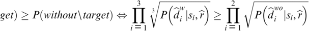


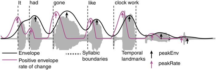
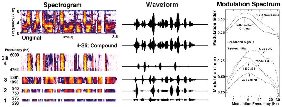

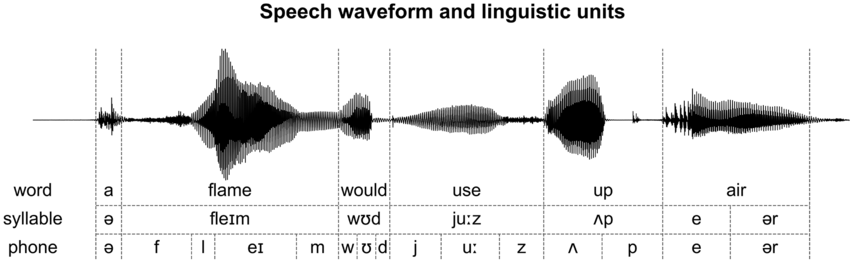

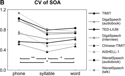


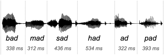


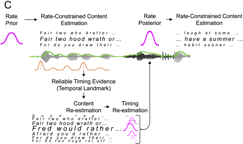
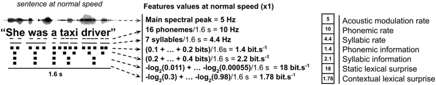
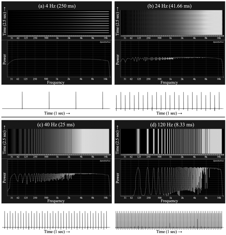
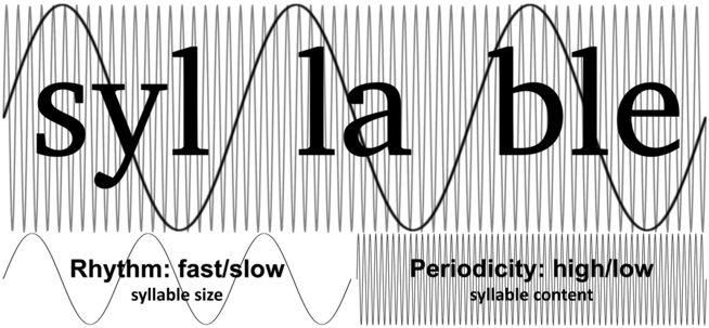

 Open access