


1. INTRODUCTION
Pulsar navigation, proposed by Downs (Reference Downs1974), is an autonomous navigation technology that utilises the periodic signals from remote pulsars to perform self-positioning. With the characteristics of independence and wide availability, pulsar navigation is particularly suitable for the fields of deep-space exploration. Among various pulsar sources, the X-ray pulsar is of great potential as small-sized detectors can be employed for navigation.
The recent decade has seen many studies in X-ray pulsar navigation, including the pulsar database, phase delay estimation, and resolution of periodic ambiguity, etc. For example, Sala et al. (Reference Sala, Urruela, Villares, Estalella and Paredes2004) analysed the feasibility of pulsar navigation in a report for the European Space Agency (ESA). They introduced a Maximum Likelihood method to estimate the time delay, which provides unbiased minimum variance estimations with mean square error approaching the Cramer-Rao Lower Bound. Sheikh and Pines (Reference Sheikh and Pines2006) proposed a new approach that provides corrections to estimated spacecraft position and achieved 200 m or less errors of positioning in numerical simulation. In Emadzadeh et al. (Reference Emadzadeh, Golshan and Speyer2009), as well as Emadzadeh and Speyer (Reference Emadzadeh and Speyer2010), epoch folding was put forward to obtain the empirical rate function and a non-linear least-squares estimator was proposed to evaluate the time delay, which has less complexity than the Maximum Likelihood estimator. Later, in Emadzadeh and Speyer (Reference Emadzadeh and Speyer2011a), a cross-correlation method for time delay estimation was proposed and its performance against the Cramer-Rao lower bound was analysed.
The key measurement of X-ray pulsar navigation, whether used for absolute positioning or relative positioning, is the time delay, which is obtained from the phase delay of the pulsar signal. Generally, there are three methods to estimate the phase delay: cross-correlation estimator, non-linear least squares estimator and maximum-likelihood estimator (Emadzadeh and Speyer, Reference Emadzadeh and Speyer2011b). A main problem of these estimators lies in the requirement to optimise non-convex functions, which will introduce a heavy computational burden. Considering that the process of autonomous navigation is realised by the computers on the spacecraft, a low-computational-complexity navigation algorithm is required for on board implementation.
In this paper, a new method for phase delay estimation is proposed, which is based on the time-shift property of a Discrete Fourier Transformation (DFT). The main advantage of this method is that the computational complexity of phase delay estimation can be greatly reduced, and with the utilisation of delta-function approximation, the computational cost as well as the memory cost can be further decreased.
The remainder of the paper is organised as follows: in Section 2, the process of epoch folding is reviewed and the computational complexities of the existing estimators are analysed. Then a DFT-based method for phase delay estimation is proposed in Section 3. Section 4 presents a numerical simulation to compare the performance of the proposed method and the cross-correlation estimator. Finally, a conclusion of the paper is given in Section 5.
2. A REVIEW OF EPOCH FOLDING AND ESTIMATORS
2.1. Fundamentals of pulsar navigation
The fundamentals of pulsar navigation can be expressed by the following equation
 $${{\bi r}_{{\bi 12}}} \cdot {\bi n} = c \cdot ({t_e} - \Delta t)$$
where r12 is the relative position vector between two spacecraft, n is the unit vector in the direction of the pulsar, c is the speed of light, t e is the time delay of pulsar arrival between two spacecraft, and Δt is the clock error. In the navigation process, the value of time delay is obtained by estimating the phase delay of pulsar signals.
2.2. Epoch folding procedure
Epoch folding is usually the first step to estimate the phase delay. In this subsection, a brief review of the epoch folding procedure is given.
To describe the rate of photons arrival, an overall rate function λ(t) is defined by (Golshan and Sheikh, Reference Golshan and Sheikh2007)
 $$\lambda (t) = {\lambda _b} + {\lambda _s}h(\varphi (t))$$
where λ b is a background arrival rate, λ s is a source arrival rate, h(ϕ) is the periodic pulsar profile, and ϕ(t) is the phase of the pulsar signal.
Epoch folding is the procedure that recovers the X-ray pulsar intensity density function from the measured photons' Times Of Arrival (TOAs). This procedure was formulated mathematically by Emadzadeh et al. (Reference Emadzadeh, Golshan and Speyer2009).
Assume that the spacecraft continually observes a pulsar for N P pulsar periods, and a pulsar period is divided into N b bins equally. So the length of each bin is T b = P/N b, where P is the period of the pulsar. Let c(t i) represent the number of photons in the ith bin whose centre is t i, then the empirical rate function can be written as (Emadzadeh and Speyer, Reference Emadzadeh, Golshan and Speyer2009)
 $$\hat \lambda ({t_i}) = \displaystyle{1 \over {{N_P}{T_b}}}\sum\limits_{\,j = 1}^{{N_P}} {{c_j}({t_i})} $$
and it can be proved that for a long observation time T obs,where  $\hat n({t_i})$ is an uncorrelated noise that satisfies
 $$E[\hat n({t_i})] = 0$$
 $${\mathop{\rm var}} [\hat n({t_i})] = \displaystyle{{{N_b}} \over {{T_{obs}}}}\lambda ({t_i})$$
The overall rate function λ(t) can be regarded as a probability density function of the arrival photons. The purpose of epoch folding is to recover the probability density function using the frequency distribution histogram of the samples (i.e., TOAs of photons).
Figure 1 shows a typical frequency distribution histogram, where a photon (black spot) is represented by a rectangle with width of T b and a unit height. By adding up all these rectangles, we can obtain the empirical rate function  $\hat \lambda ({t_i})$.

Figure 1. A frequency distribution histogram.
Assume that the number of photons arriving during the observation time is N. For every photon, it is necessary to find the exact bin it falls in and update the corresponding  ${c_j}({t_i})$. So, the computation complexity of the epoch folding procedure is $O(N)$. In Section 3.2, it will be shown that representing a photon by a delta-function instead of a rectangle can diminish the computational complexity.
2.3. Phase delay estimators
In this subsection, three methods to estimate the phase delay are presented: maximum-likelihood estimator, non-linear least squares estimator and cross-correlation estimator.
The fundamental of maximum-likelihood estimator is to find a phase delay that maximises the joint probability of the observed TOAs (Sala et al., Reference Sala, Urruela, Villares, Jordi and Sebastia2008). In practice, log-likelihood is commonly used
 $$\Psi (\varphi ) = \sum\limits_{i = 1}^N {\ln (\lambda ({t_i};\varphi ))} $$
And the estimation of phase delay is
 $$\hat \varphi = \arg \max \Psi (\varphi )$$
which requires optimising a non-convex function, and the grid search is a general choice. Assume that we search N b candidates of ϕ, and for every ϕ, ψ(ϕ) should be computed, which requires a computational complexity of  $O(N{N_b})$. Besides, finding the maximum of all the ψ(ϕ)s needs $O({N_b})$ complexity. Therefore, the total computational complexity is O(NN b + N b) for the maximum-likelihood estimator.
The non-linear least squares estimator minimises a so-called cost function (Emadzadeh et al., Reference Emadzadeh, Golshan and Speyer2009)
 $$J(\varphi ) = \sum\limits_{n = 1}^{{N_b}} {{{(\hat \lambda (n;\varphi ) - \lambda (n))}^2}} $$
where λ(n) and  $\hat \lambda (n;\varphi )$ are the discretizations of the overall and empirical rate functions, respectively. The estimation of phase delay is
 $$\hat \varphi = \arg \min J(\varphi )$$
This process needs epoch folding with the complexity of O(N), and for every ϕ we should compute J(ϕ), which requires a complexity of O(N b2). To find the minimal of J(ϕ), O(N b) a computational cost is generated. Thus, the total computational complexity of the non-linear least squares estimator is O(N + N b2 + N b).
The cross-correlation estimator maximises the cross correlation function of the overall rate function and the empirical rate function (Emadzadeh and Speyer, Reference Emadzadeh and Speyer2011a), which can be expressed as
 $$R(\varphi ) = \int_{ - \infty }^\infty {{\lambda ^*}(t)\hat \lambda (t;\varphi )dt} $$
And the estimation of phase delay is
 $$\hat \varphi = - \arg \max R(\varphi )$$
In practice, DFT is usually employed to compute the cross correlation function
 $$\eqalign{{\Lambda _1}(k) =\, & DFT[\lambda (n)],\;{\Lambda _2}(k) = DFT[\hat \lambda (n)], \cr & \quad R(n ) = IDFT[{\Lambda _1}(k){\ast} {{\Lambda _2}^{\ast}}(k)]} $$
This process also needs epoch folding, and the DFT process requires a computational cost of  $O({N_b}\log {N_b})$ with the fast Fourier transformation (FFT) algorithm (Cooley and Tukey, Reference Cooley and Tukey1965). Then the maximum of R(n) can be found with a complexity of O(N b). So the total complexity is $O(N + {N_b}\log {N_b} + {N_b})$ for the cross-correlation estimator.
Table 1 summarises the computational complexities of the above three estimators. It can be seen that when the number of photons N and the number of bins N b are large, the cross-correlation estimator has the least computational cost.
Table 1. Computational complexities of estimators.

3. A DFT-BASED METHOD FOR PHASE DELAY ESTIMATION
3.1. Proposal of the DFT based method
In this section, a method for phase delay estimation based on the time-shift property of DFT is proposed.
According to the time-shift property of DFT, a cyclic shift of a sequence in time domain is equivalent to a phase shift in frequency domain. That is, if
 $$\left\{ {\matrix{ {X(k) = DFT[x(n)]} \cr {y(n) = x{{(n - m)}_N}} \cr}} \right.$$
then,
 $$DFT[\,y(n)] = X(k)\exp \left( { - j\displaystyle{{2\pi} \over N}mk} \right)$$
where j 2 = −1.
As a consequence, the time shift in time domain m can be obtained by computing the phase shift  $ - \displaystyle{{2\pi} \over N}mk$ in frequency domain.
The intention of phase delay estimation is to find a phase delay  $\hat \varphi $ in time domain such that
 $$\hat \lambda (n) = \lambda {(n - \hat \varphi )_{{N_b}}} + \hat n(n)$$
where  $\hat n(n)$ is an uncorrelated noise.
Assume that
 $$\left\{ {\matrix{ {{\Lambda _1}(k) = DFT[\lambda (n)]} \cr {{\Lambda _2}(k) = DFT[\hat \lambda (n)]} \cr}} \right.$$
and according to the time-shift property of DFT,
 $$DFT[\lambda (n - \hat \varphi )] = {\Lambda _1}(k)\exp \left( { - j\displaystyle{{2\pi} \over {{N_b}}}\hat \varphi k} \right)$$
It can then be obtained by performing a DFT on Equation (16) that
 $${\Lambda _2}(k) = {\Lambda _1}(k)\exp \left( { - j\displaystyle{{2\pi} \over {{N_b}}}\hat \varphi k} \right) + N(k),\quad 0 \le k \le {N_b} - 1$$
where  $N(k) = DFT[\hat n(n)]$ is the DFT of the noise, and Equation (19) is valid for any $k \in [0,{N_b} - 1]$.
So, the estimation of phase delay is
 $$\hat \varphi = - \displaystyle{{{N_b}} \over {2\pi k}}ang\displaystyle{{{\Lambda _2}(k)} \over {{\Lambda _1}(k)}}$$
where  $ang\displaystyle{{{\Lambda _2}(k)} \over {{\Lambda _1}(k)}}$ is the phase angle of the complex $\displaystyle{{{\Lambda _2}(k)} \over {{\Lambda _1}(k)}}$, and Equation (20) is also valid for any $k \in [0,{N_b} - 1]$.
Instead of computing the whole DFT sequence, this method only computes Λ1(k) and Λ2(k) of a certain  $k \in [0,{N_b} - 1]$ to obtain the estimation of phase delay. Using the definition of DFT, it can be obtained that
 $${\Lambda _2}(k) = \sum\limits_{n = 1}^{{N_b}} {\hat \lambda (n)\exp \left( { - j\displaystyle{{2\pi} \over {{N_b}}}nk} \right)} $$
With the Horner Algorithm (Horner, Reference Horner1819), the computations of Λ1(k) and Λ2(k) by Equation (21) only require O(N b) complexity. This process also needs epoch folding with the complexity of O(N). As a result, the total computational complexity is O(N + N b), smaller than that of estimators presented in Section 2.
As stated above that for any  $k \in [0,{N_b} - 1]$, the phase delay can be estimated by Equation (20). The best estimation of phase delay can be obtained by choosing the ‘best’ k which minimises the effect of the noise $\hat n(n)$.
Equation (19) leads to
 $$\displaystyle{{{\Lambda _2}(k)} \over {{\Lambda _1}(k)}} = \exp \left( { - j\displaystyle{{2\pi} \over {{N_b}}}\hat \varphi k} \right) + \displaystyle{{N(k)} \over {{\Lambda _1}(k)}}$$
Since the amplitude and phase angle of N(k) are random, the k to be chosen is the one that maximises the amplitude of Λ1(k).
 $$k = \arg \max \vert{\Lambda _1}(k)\vert$$
In this way, the effect of  $\displaystyle{{N(k)} \over {{\Lambda _1}(k)}}$ can be minimised.
Searching for the ‘best’ k requires the computation of the whole DFT sequence of λ(n), but the overall rate function λ(n) is ‘known’ before the spacecraft launched, so the ‘best’ k and corresponding Λ1(k) can be found ‘offline’, which means the computations of k and corresponding Λ1(k) impose no complexity for on board computation.
3.2. Delta-Function Approximation
Since k and Λ1(k) are obtained ‘offline’, during the process of navigation, only Λ2(k) is computed using Equation (21), where the empirical rate function  $\hat \lambda (n)$ can be obtained through the epoch folding process. In this subsection, a delta-function approximation is put forward to replace epoch folding. With this approximation, one can directly obtain Λ2(k) in a lower complexity.
As discussed before, the epoch folding procedure regards photons as rectangles and uses a histogram to estimate the overall probability density function. Similarly, we can regard the photons as delta functions
 $$\delta (t - \mu ) = \left\{ {\matrix{ {\infty, t - \mu = 0} \cr {0,t - \mu \ne 0} \cr}} \right.$$
whose centres are the ‘fractions’ of TOAs. Assume that the TOA of a photon contains  ${N_P}$ pulsar periods, then the ‘fraction’ is defined as
 $$\mu = TOA - {N_P}P$$
The empirical rate function  $\hat \lambda (t)$ can be redefined by
 $$\hat \lambda (t) = \sum\limits_{i = 1}^N {\delta (t - {\mu _i})} $$
where μ i is the ‘fraction’ of the ith photon.
By noting the time-shift property of DFT and DFT [δ(t)] = 1, it can be derived that
 $$DFT[\delta (t - \mu )] = \exp ( - jk\mu )$$
With the use of DFT on Equation (26), it can be obtained that
 $${\Lambda _2}(k) = \sum\limits_{i = 1}^N {{e^{ - jk{\mu _i}}}} $$
where μ i is the ‘fraction’ of the ith photon.
Equation (28) means that, with the delta-function approximation, the computation of empirical rate function  $\hat \lambda (t)$ can be skipped and Λ2(k) can be obtained directly from TOAs of photons. As a consequence, the total computational cost can be reduced to O(N), significantly less than that of the proposed method in Section 3.1. On the other hand, employing the delta-function approximation will not significantly lose accuracy, which will be shown in Section 4.
Furthermore, with the delta-function approximation, the memory cost is also decreased, because there is no need to save the empirical rate function  $\hat \lambda (n)$, whose length is N b.
3.3. Scheme of the proposed method
Based on the above description, the scheme of the proposed method is clarified in this subsection.
When k > 1, the phase angle of the complex  $\displaystyle{{{\Lambda _2}(k)} \over {{\Lambda _1}(k)}}$ may exceed 2π, meaning that the 2Mπ part of $ang\displaystyle{{{\Lambda _2}(k)} \over {{\Lambda _1}(k)}}$ cannot be found directly by using trigonometric calculation. Consequently, the estimation of phase delay cannot be obtained directly through Equation (20) and it should be rewritten as
 $$\hat \varphi = - \displaystyle{{{N_b}} \over {2\pi k}}\left( {ang\displaystyle{{{\Lambda _2}(k)} \over {{\Lambda _1}(k)}} + 2M\pi} \right)$$
where M is an integer.
To solve this problem, let us set k = 1 at first, and make a ‘rough’ estimation of  $\hat \varphi $ by
 $${\hat \varphi _1} = - \displaystyle{{{N_b}} \over {2\pi}} ang\displaystyle{{{\Lambda _2}(1)} \over {{\Lambda _1}(1)}}$$
Then, substitute the ‘rough’ estimation into Equation (29) to solve M
 $$M = round\left( { - \displaystyle{{k{{\hat \varphi} _1}} \over {{N_b}}} - \displaystyle{1 \over {2\pi}} ang\displaystyle{{{\Lambda _2}(1)} \over {{\Lambda _1}(1)}}} \right)$$
where round(x) is the arithmetical operation to find the closest integer of x. Using the solution of M, the estimation of phase delay  $\hat \varphi $ can be finally determined by Equation (29).
The scheme of the DFT-based method with the delta-function approximation can be summarised as follows:
(1) Offline procedure:
a) Compute Λ1(k) = FFT [λ(n)]
b) Find k = arg max[Λ1(k)]
(2) Online procedure:
a) Compute ${\Lambda _2}(1) = \sum\limits_{i = 1}^N {{e^{ - j{\mu _i}}}} $, where μ = TOA−N PP
b) Compute
${\Lambda _2}(k) = \sum\limits_{i = 1}^N {{e^{ - jk{\mu _i}}}} $c) ‘Rough’ estimation
${\hat \varphi _1} = - \displaystyle{{{N_b}} \over {2\pi}} ang\displaystyle{{{\Lambda _2}(1)} \over {{\Lambda _1}(1)}}$d) Find
$M = round\left( { - \displaystyle{{k{{\hat \varphi} _1}} \over {{N_b}}} - \displaystyle{1 \over {2\pi}} ang\displaystyle{{{\Lambda _2}(1)} \over {{\Lambda _1}(1)}}} \right)$e)
$\hat \varphi = - \displaystyle{{{N_b}} \over {2\pi k}}\left( {ang\displaystyle{{{\Lambda _2}(k)} \over {{\Lambda _1}(k)}} + 2M\pi } \right)$

4. NUMERICAL SIMULATION
As stated above, when the number of photons N and the number of bins N b are large, the cross-correlation estimator has the lowest computational complexity (O(N + N b log N b + N b)) among the three estimators presented in Section 2. By using the DFT-based method, the computational complexity can be effectively reduced to O(N + N b), and with the aid of delta-function approximation, it can be further lowered to O(N). In this section, a numerical simulation is made to compare the performance of the DFT-based method and the cross-correlation estimator.
In the simulation, we choose N b = 1048576, and N ranges from 1024 to 1048576. The phase delay is estimated using pulsars B0833-45 and J1420-6048. By using an Intel(R) Xeon(R) 3·60 GHz CPU processor. The resulting computation time and phase delay estimation errors are listed in Tables 2 and 3.
Table 2. The simulation result of pulsar B0833-45.
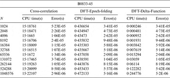
Table 3. The simulation result of pulsar J1420-6048.

To illustrate the comparison more clearly, Figure 2 shows the time delay estimation errors of the three methods. From the results, it can be seen that
• The phase delay estimation error of the DFT-based method is generally in the same order as that of the cross-correlation estimator.
• It takes the cross-correlation estimator about 15 seconds CPU time to estimate a phase delay, while the DFT-based method only takes a CPU time of about 0·4 seconds.
• With the use of delta-function approximation, the time consumption of the DFT-based method can be further decreased without loss of accuracy.

Figure 2. Time delay estimation error. Left:B0833-45. Right: J1420-6048.
5. CONCLUSION
This paper reviews some commonly used phase delay estimators in X-ray pulsar navigation. Considering the high computational complexities of these existing estimators, a new method for phase delay estimation is proposed, which is based on the time-shift property of DFT.
In the proposed method, only a specific term of the DFT sequence, instead of the whole DFT sequence is computed, which accelerates the estimation of phase delay. Besides that, a delta-function approximation is put forward to replace the epoch folding process. With this approximation, both the time complexity and memory cost can be greatly reduced.
Finally, a numerical simulation was conducted to evaluate the performance of the proposed method. The simulation results indicate that the DFT-based method with delta-function approximation has the lowest computational complexity and the same-order accuracy in phase delay estimation. Due to its efficiency and superiority, the proposed method will be more suitable for future on board application.
ACKNOWLEDGMENTS
This work was carried out with financial support from the National Basic Research Program 973 of China (2013CB834103).


