


1 Introduction
Current inertial confinement fusion (ICF) indirect-drive ablative Rayleigh–Taylor instability andradiative opacity experiment targets field on ShenGuang III and II. With few such experiments, target fabrication and alignment accuracy, enhanced metrology and advanced component machining will be even more important. The future target designs are also becoming more complex and more stringent in terms of assembly precision. A key specification of these targets is the spatial angle, which makes it impossible to assemble microtarget by manual assembly[Reference Ding, Jiang and Liu1–Reference Miao and Yuan3]. The internal and external researches have shown that using the semi-automatic assembly system based on microscopic vision can improve the assembly precision and stabilization[Reference Tamadazte, Sounkalo and Guillaume4–Reference Chu, Mills and Cleghorn6].
The majority of semi-automatic operations in the macroworld rely on accurate robots that play back recorded motions. However, this form of open-loop manipulation is not suitable at the microscale target components due to the increased precision requirements and the vastly different mechanics of manipulation. In recent years, the availability of high resolution cameras and powerful microprocessors have made possible for the vision systems to play a key role in the automatic microsystems assembly field. In Refs. [Reference Fatikow, Buerkle and Seyfried7–Reference Ralis, Vikramaditya and Nelson10], it was shown that microvision-based precise assembly method is an appropriate solution in the automation of micromanipulation and microassembly tasks. In Refs. [Reference Tamadazte, Le Fort-Piat and Marchand11, Reference Tamadazte, Le Fort-Piat and Sounkalo12], the authors proposed a 3D vision-based microassembly method for 3D microelectromechanical systems (MEMS)[Reference Chang, Liimatainen, Routa and Zhou13] and reported that the positioning accuracy of microchips on patterns with jagged edges using hybrid microassembly technique[Reference Yesin and Nelson14] presented an alternative method for visual tracking of microcomponents using a CAD model. However, a large part of the microassembly systems presented in the literature are concerned about the position alignment accuracy of micropart; few works deal with the use of pose-based visual control techniques and concern the spatial angle alignment accuracy[Reference Tamadazte, Le Fort-Piat and Sounkalo12].
In this paper, we present a new spatial angle assembly method of the ICF microtarget, using target parts 3D model based on dual orthogonal camera vision. Our goal is to develop a generally applicable spatial angle measuring method that is better suited for the flexible automation of target assembly processes. Section 2 describes the target assembly system structure. Section 3 presents the method of spatial angle on-line measurement. Section 4 discusses the error of the spatial angle assembly method. Sections 5 and 6 present some experimental results obtained and discussions about them.
2 Spatial angle microassembly system design
We constructed a semi-automatic assembly system to improve target spatial angle assembly accuracy. It consists of control system, micromanipulate system, gripper system and visual feedback system, as shown in Figure 1. The system can implement some of the following functions: gripping function, location function, detection function, figure-comparing function, posture adjustment function and assembly function.
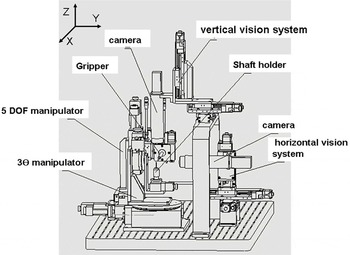
Figure 1. Spatial angle assembly system.
The visual feedback system utilizes a dual-axis camera viewing system shown in Figure 1. Every camera viewing system is composed of light source, zoom lens and CCD camera. The specification model of CCD and zoom lens are Baumer SXG20 and Navitar 12X, respectively. The upper vertical camera is the main line of sight for vertical viewing of target parts, and the calculated orientation by comparing the target image with the $\mathit{XY}$
projection of target’s 3D model. The horizontal camera is used to get the left view and the calculated orientation by comparing the target image with the
$\mathit{XY}$
projection of target’s 3D model. The horizontal camera is used to get the left view and the calculated orientation by comparing the target image with the $\mathit{YZ}$
projection of target’s 3D model. Every camera mount on the
$\mathit{YZ}$
projection of target’s 3D model. Every camera mount on the $\mathit{XYZ}$
electric linear stages, which is used to switch assembly position and produce a 100 mm
$\mathit{XYZ}$
electric linear stages, which is used to switch assembly position and produce a 100 mm $\times$
100 mm
$\times$
100 mm $\times$
150 mm working volume for flexibility, deal with overall current targets and accommodating future needs.
$\times$
150 mm working volume for flexibility, deal with overall current targets and accommodating future needs.
The structure of micromanipulate system used for the target assembly process is illustrated in Figure 2. Its structure is separated into two independent manipulators: a 5 degree of freedom (DOF) ( $xyz\unicode[STIX]{x1D703}\unicode[STIX]{x1D711}$
) manipulator and a
$xyz\unicode[STIX]{x1D703}\unicode[STIX]{x1D711}$
) manipulator and a $3\unicode[STIX]{x1D703}$
manipulator (their parameters are shown in Table 1). The 5 DOF (
$3\unicode[STIX]{x1D703}$
manipulator (their parameters are shown in Table 1). The 5 DOF ( $xyz\unicode[STIX]{x1D703}\unicode[STIX]{x1D711}$
) manipulator is composed of three electric linear stages, that create a 100 mm
$xyz\unicode[STIX]{x1D703}\unicode[STIX]{x1D711}$
) manipulator is composed of three electric linear stages, that create a 100 mm $\times$
100 mm
$\times$
100 mm $\times$
150 mm working volume, and two electric rotary stages create pitch and roll correction for the alignment of assembled backlight components held by the microgripper at the end of the manipulator. The
$\times$
150 mm working volume, and two electric rotary stages create pitch and roll correction for the alignment of assembled backlight components held by the microgripper at the end of the manipulator. The $3\unicode[STIX]{x1D703}$
manipulator is composed of three rotary stages that work together to orient the main component of target to any desired spatial attitude. The
$3\unicode[STIX]{x1D703}$
manipulator is composed of three rotary stages that work together to orient the main component of target to any desired spatial attitude. The $\unicode[STIX]{x1D703}_{z}$
’ rotary stage is controlled separately to allow any side of the aligned target to be positioned toward the 5 DOF (
$\unicode[STIX]{x1D703}_{z}$
’ rotary stage is controlled separately to allow any side of the aligned target to be positioned toward the 5 DOF ( $xyz\unicode[STIX]{x1D703}\unicode[STIX]{x1D711}$
) manipulator.
$xyz\unicode[STIX]{x1D703}\unicode[STIX]{x1D711}$
) manipulator.
Figure 2. The mechanical structure of the micromanipulate system.
Table 1. Micromanipulate system specifications.
3 Spatial angle on-line measurement method
During target assembly operations, a vision feedback model is set to observe assembly process in real time, and the image processing is used to implement part’s alignment process. Image processing methods such as image preprocessing, feature extraction, edge recognition and detection are usually used[Reference Hériban, Thiebault and Gauthier15–Reference Oku, Ishii and Ishikawa17]. But in real world, these methods are not better suited for the changing of the target’s structure and component. For the problem, this paper designs an algorithm based on 3D model to achieve space angle alignment. The flow of alignment process is shown in Figure 3.

Figure 3. The flow chart of spatial angle measuring.
As shown in Figure 3, the 3D model of target is built by emulation software, which can have no deviation. The perpendicular 2D projection pictures are then selected from it; in order to exchange the data between different software, the projection pictures are saved in DXF file format. In the operating system, an algorithm is designed to read DXF file and draw the projection figure on the vision interface. During the target assembly manipulating, the projection figure is depicted in a statement of proportion to the image gathered from microscopic vision based on the pixel equivalent. By comparing the real-time image with the redrawing 2D projection, we can achieve the spatial angle alignment within the given division by vision feedback control.
4 Analysis on assembly precision
The target microassembly system used was the visual servo control method and the resolution of rotary stage of micromanipulate system is better than the resolution of dual-axis camera viewing system, so the spatial assembly precision is determined by the measurement accuracy.
The measurement accuracy of the spatial angle $E$
is limited by the error
$E$
is limited by the error $E_{i}$
which is generated by image comparison, the error
$E_{i}$
which is generated by image comparison, the error $E_{c}$
of calibration between horizontal visual and vertical visual, and the error
$E_{c}$
of calibration between horizontal visual and vertical visual, and the error $E_{d}$
of redrawing 2D projection.
$E_{d}$
of redrawing 2D projection.
 $$\begin{eqnarray}\displaystyle E=\sqrt{E_{i}^{2}+E_{c}^{2}+E_{d}^{2}}. & & \displaystyle\end{eqnarray}$$

Figure 4. Spatial angle.
The spatial angle of the strict requirements in the target assembly can be converted into the angle between two vectors. In the spatial angle on-line measuring system, the vector $\overrightarrow{I}$
of the target’s part can be described as
$\overrightarrow{I}$
of the target’s part can be described as $(\cos \unicode[STIX]{x1D6FD}^{\prime },\cos \unicode[STIX]{x1D6FC}^{\prime },\cos \unicode[STIX]{x1D6FE}^{\prime })$
shown in Figure 4.
$(\cos \unicode[STIX]{x1D6FD}^{\prime },\cos \unicode[STIX]{x1D6FC}^{\prime },\cos \unicode[STIX]{x1D6FE}^{\prime })$
shown in Figure 4.
By using the horizontal CCD and the vertical CCD, we can get the angle of the vector $\overrightarrow{I}$
’s projection in
$\overrightarrow{I}$
’s projection in $\mathit{YZ}$
and
$\mathit{YZ}$
and $\mathit{XY}$
coordinate plane, respectively. Through querying the spatial angle calculation table in Ref. [Reference Bolu18], we can get the calculating formula
$\mathit{XY}$
coordinate plane, respectively. Through querying the spatial angle calculation table in Ref. [Reference Bolu18], we can get the calculating formula
 $$\begin{eqnarray}\displaystyle & \displaystyle \tan \unicode[STIX]{x1D6FC}=\tan \unicode[STIX]{x1D6FC}_{w}\cdot \sin \unicode[STIX]{x1D6FD}_{H}, & \displaystyle\end{eqnarray}$$
 $$\begin{eqnarray}\displaystyle & \displaystyle \tan \unicode[STIX]{x1D6FD}=\sqrt{\cot ^{2}\unicode[STIX]{x1D6FD}_{H}+\tan ^{2}\unicode[STIX]{x1D6FC}_{w}}, & \displaystyle\end{eqnarray}$$
 $$\begin{eqnarray}\displaystyle & \displaystyle \tan \unicode[STIX]{x1D6FE}=\cos \unicode[STIX]{x1D6FC}_{w}/\tan \unicode[STIX]{x1D6FD}_{H}. & \displaystyle\end{eqnarray}$$
The values of $\unicode[STIX]{x1D6FC}_{w}$
and
$\unicode[STIX]{x1D6FC}_{w}$
and $\unicode[STIX]{x1D6FD}_{H}$
can be measured by the images of horizontal CCD and vertical CCD, respectively, so we can easily get the coordinate value of the vector in the Cartesian coordinate system.
$\unicode[STIX]{x1D6FD}_{H}$
can be measured by the images of horizontal CCD and vertical CCD, respectively, so we can easily get the coordinate value of the vector in the Cartesian coordinate system.
 $$\begin{eqnarray}\displaystyle \cos \unicode[STIX]{x1D6FC}^{\prime } & = & \displaystyle \sqrt{\frac{1}{1+\tan ^{2}\unicode[STIX]{x1D6FC}}}\bullet \cos \unicode[STIX]{x1D6FD}_{H}\nonumber\\ \displaystyle & = & \displaystyle \frac{\cos \unicode[STIX]{x1D6FD}_{H}}{\sqrt{1+\tan ^{2}\unicode[STIX]{x1D6FC}_{W}\bullet \sin ^{2}\unicode[STIX]{x1D6FD}_{H}}},\end{eqnarray}$$
 $$\begin{eqnarray}\displaystyle \cos \unicode[STIX]{x1D6FD}^{\prime } & = & \displaystyle \sqrt{\frac{1}{1+\tan ^{2}\unicode[STIX]{x1D6FC}}}\bullet \sin \unicode[STIX]{x1D6FD}_{H}\nonumber\\ \displaystyle & = & \displaystyle \frac{\sin \unicode[STIX]{x1D6FD}_{H}}{\sqrt{1+\tan ^{2}\unicode[STIX]{x1D6FC}_{W}\bullet \sin ^{2}\unicode[STIX]{x1D6FD}_{H}}},\end{eqnarray}$$
 $$\begin{eqnarray}\displaystyle \cos \unicode[STIX]{x1D6FE}^{\prime } & = & \displaystyle \sqrt{\frac{1}{1+\tan ^{2}\unicode[STIX]{x1D6FE}}}\bullet \cos \unicode[STIX]{x1D6FC}_{W}\nonumber\\ \displaystyle & = & \displaystyle \frac{\tan \unicode[STIX]{x1D6FD}_{H}\bullet \cos \unicode[STIX]{x1D6FC}_{W}}{\sqrt{\tan ^{2}\unicode[STIX]{x1D6FD}_{H}+\cos ^{2}\unicode[STIX]{x1D6FC}_{W}}}.\end{eqnarray}$$
Suppose the axis vectors of the two assembling target parts are $\overrightarrow{I_{1}}$
and
$\overrightarrow{I_{1}}$
and $\overrightarrow{I_{2}}$
, the angle between them can be calculated by the following formula:
$\overrightarrow{I_{2}}$
, the angle between them can be calculated by the following formula:
 $$\begin{eqnarray}\displaystyle & & \displaystyle \cos \langle \overrightarrow{I}_{1},\overrightarrow{I}_{2}\rangle =\frac{\overrightarrow{I}_{1}\cdot \overrightarrow{I}_{2}}{|\overrightarrow{I_{1}}|\,|\overrightarrow{I_{2}}|}\nonumber\\ \displaystyle & & \displaystyle \quad =\frac{\cos \unicode[STIX]{x1D6FC}_{1}^{\prime }\cdot \cos \unicode[STIX]{x1D6FC}_{2}^{\prime }+\cos \unicode[STIX]{x1D6FD}_{1}^{\prime }\cdot \cos \unicode[STIX]{x1D6FD}_{2}^{\prime }+\cos \unicode[STIX]{x1D6FE}_{1}^{\prime }\cdot \cos \unicode[STIX]{x1D6FE}_{2}^{\prime }}{\sqrt{\cos \unicode[STIX]{x1D6FC}_{1}^{\prime 2}+\cos \unicode[STIX]{x1D6FD}_{1}^{\prime 2}+\cos \unicode[STIX]{x1D6FE}_{1}^{\prime 2}}\cdot \sqrt{\cos \unicode[STIX]{x1D6FC}_{2}^{\prime 2}+\cos \unicode[STIX]{x1D6FD}_{2}^{\prime 2}+\cos \unicode[STIX]{x1D6FE}_{2}^{\prime }}}.\nonumber\\ \displaystyle & & \displaystyle\end{eqnarray}$$
In this paper, we designed a method of measuring the spatial angle, that compared the real-time image with the redrawing 2D projection. The measurement of the angle accuracy is limited by the resolution of the camera viewing system. The resolution of the CCD is 1600 $\times$
1200 and field of view is 8 mm
$\times$
1200 and field of view is 8 mm $\times$
6 mm, so the resolution of the camera viewing system is about
$\times$
6 mm, so the resolution of the camera viewing system is about $2.5~\unicode[STIX]{x03BC}\text{m}$
that half of the pixel value. It means that when the length is about 1 mm of the target parts, it leads to the maximum error
$2.5~\unicode[STIX]{x03BC}\text{m}$
that half of the pixel value. It means that when the length is about 1 mm of the target parts, it leads to the maximum error $E_{i}$
of about
$E_{i}$
of about $0.143^{\circ }$
.
$0.143^{\circ }$
.
Figure 5. Coordinate system.
Due to the installation accuracy of the visual feedback system and other reasons, it is difficult to ensure that the measurement coordinate system of the dual-axis camera viewing system and the 3D modeling coordinate system is exactly the same. As is shown in Figure 5, for the vertical CCD, it may be along the $\mathit{XY}$
axis to produce the translation deviation and the deviation of rotation around the
$\mathit{XY}$
axis to produce the translation deviation and the deviation of rotation around the $Z$
direction. For the horizontal CCD it may be along the
$Z$
direction. For the horizontal CCD it may be along the $\mathit{YZ}$
axis to produce the translation deviation and the deviation of rotation around the
$\mathit{YZ}$
axis to produce the translation deviation and the deviation of rotation around the $X$
direction. Although it is calibrated by adopted Equation (9) in this paper, it is difficult to avoid errors. Tested by using standard hexahedron, the calibration error
$X$
direction. Although it is calibrated by adopted Equation (9) in this paper, it is difficult to avoid errors. Tested by using standard hexahedron, the calibration error $\unicode[STIX]{x1D6E5}_{Ec}\unicode[STIX]{x1D6FC}_{w}$
of the horizontal CCD is
$\unicode[STIX]{x1D6E5}_{Ec}\unicode[STIX]{x1D6FC}_{w}$
of the horizontal CCD is $0.06^{\circ }$
and the error
$0.06^{\circ }$
and the error $\unicode[STIX]{x1D6E5}_{Ec}\unicode[STIX]{x1D6FD}_{H}$
of the vertical CCD is
$\unicode[STIX]{x1D6E5}_{Ec}\unicode[STIX]{x1D6FD}_{H}$
of the vertical CCD is $0.07^{\circ }$
.
$0.07^{\circ }$
.
 $$\begin{eqnarray}\displaystyle \left[\begin{array}{@{}c@{}}\unicode[STIX]{x1D6E5}x\\ \unicode[STIX]{x1D6E5}y\\ \unicode[STIX]{x1D6E5}z\\ \unicode[STIX]{x1D6E5}\unicode[STIX]{x1D6E9}_{x}\\ \unicode[STIX]{x1D6E5}\unicode[STIX]{x1D6E9}_{y}\\ \unicode[STIX]{x1D6E5}\unicode[STIX]{x1D6E9}_{z}\end{array}\right] & = & \displaystyle (J^{T}J)^{-1}J^{T}\left[\begin{array}{@{}c@{}}\unicode[STIX]{x1D6E5}u_{c11}\\ \unicode[STIX]{x1D6E5}v_{c11}\\ \unicode[STIX]{x1D6E5}\unicode[STIX]{x1D719}_{c11}\\ \unicode[STIX]{x1D6E5}u_{c21}\\ \unicode[STIX]{x1D6E5}v_{c21}\\ \unicode[STIX]{x1D6E5}\unicode[STIX]{x1D719}_{c21}\end{array}\right]\nonumber\\ \displaystyle & = & \displaystyle J^{+}\left[\begin{array}{@{}c@{}}\unicode[STIX]{x1D6E5}u_{c11}\\ \unicode[STIX]{x1D6E5}v_{c11}\\ \unicode[STIX]{x1D6E5}\unicode[STIX]{x1D719}_{c11}\\ \unicode[STIX]{x1D6E5}u_{c21}\\ \unicode[STIX]{x1D6E5}v_{c21}\\ \unicode[STIX]{x1D6E5}\unicode[STIX]{x1D719}_{c21}\end{array}\right],\end{eqnarray}$$
where $\unicode[STIX]{x1D6E5}u_{cij}$
,
$\unicode[STIX]{x1D6E5}u_{cij}$
, $\unicode[STIX]{x1D6E5}v_{cij}$
are increments of image coordinate, and
$\unicode[STIX]{x1D6E5}v_{cij}$
are increments of image coordinate, and $\unicode[STIX]{x1D6E5}\unicode[STIX]{x1D719}_{cij}$
is increment of direction angle.
$\unicode[STIX]{x1D6E5}\unicode[STIX]{x1D719}_{cij}$
is increment of direction angle.

Figure 6. The flow chart of redrawing 2D projection.

Figure 7. The flow chart of semi-automatic assembly process.

Figure 8. Pictures about assembly experiment.
Figure 9. Result of the assembly experiment.
During the process of the target assembly, the processing of 2D projection redrawing is shown in Figure 6. In this processing the magnification of the imaging system needs to be calibrated. There is an error in the calibration process, which leads to the deviation between the image and the actual image, which can in turn lead to the measurement error of the spatial angle during the subsequent alignment processing. In this paper, we adopt the 2 mm standard ball to calibrate the two imaging systems, and then take the 1 mm standard ball to test the error. Test results are 1.4 and $1.7~\unicode[STIX]{x03BC}\text{m}$
, which lead to the maximum angle error of about
$1.7~\unicode[STIX]{x03BC}\text{m}$
, which lead to the maximum angle error of about $0.097^{\circ }$
(
$0.097^{\circ }$
( $\unicode[STIX]{x1D6E5}_{Ed}\unicode[STIX]{x1D6FC}_{w}$
) and
$\unicode[STIX]{x1D6E5}_{Ed}\unicode[STIX]{x1D6FC}_{w}$
) and $0.08^{\circ }$
(
$0.08^{\circ }$
( $\unicode[STIX]{x1D6E5}_{Ed}\unicode[STIX]{x1D6FD}_{H}$
), respectively.
$\unicode[STIX]{x1D6E5}_{Ed}\unicode[STIX]{x1D6FD}_{H}$
), respectively.
So, the maximum measurement error of $E_{\unicode[STIX]{x1D6FC}_{W}}$
and
$E_{\unicode[STIX]{x1D6FC}_{W}}$
and $E_{\unicode[STIX]{x1D6FD}_{H}}$
are obtained:
$E_{\unicode[STIX]{x1D6FD}_{H}}$
are obtained: $E_{\unicode[STIX]{x1D6FC}_{W}}$
is
$E_{\unicode[STIX]{x1D6FC}_{W}}$
is $0.183^{\circ }$
and
$0.183^{\circ }$
and $E_{\unicode[STIX]{x1D6FD}_{H}}$
is
$E_{\unicode[STIX]{x1D6FD}_{H}}$
is $0.178^{\circ }$
. Normally, it is ensured that one of the two assembly target parts in the assembly of a part of the axis vector and projection
$0.178^{\circ }$
. Normally, it is ensured that one of the two assembly target parts in the assembly of a part of the axis vector and projection $\mathit{XOY}$
or
$\mathit{XOY}$
or $\mathit{YOZ}$
plane is parallel. Therefore, the maximum value of
$\mathit{YOZ}$
plane is parallel. Therefore, the maximum value of $E_{\unicode[STIX]{x1D6FC}_{W}}$
and
$E_{\unicode[STIX]{x1D6FC}_{W}}$
and $E_{\unicode[STIX]{x1D6FD}_{H}}$
can be selected as the measuring error of the system.
$E_{\unicode[STIX]{x1D6FD}_{H}}$
can be selected as the measuring error of the system.
5 Experiment and result
A spatial angle assembly experiment of target is accomplished by the spatial angle assembly system. Figure 7 is the flow chart of semi-automatic assembly process, and Figure 8 shows some of the process pictures in assembly experiments.
By comparing the images gathered from microscopic vision with projection pictures, we are constantly adjusting the position and pose of targets until they coincide. As shown in Figure 9(b), the maximum error of assembly is $0.45^{\circ }$
, and the minimum error is
$0.45^{\circ }$
, and the minimum error is $0.12^{\circ }$
. The result shows that the proposed assembly method is very effective and meets the requirements of angle assembly accuracy that is less than
$0.12^{\circ }$
. The result shows that the proposed assembly method is very effective and meets the requirements of angle assembly accuracy that is less than $1^{\circ }$
.
$1^{\circ }$
.
6 Conclusion
In this paper, a spatial angle microassembly system was investigated by considering the kinematics, spatial angle measuring on-line and motion control in an integrated way. To address the special angular requirements of $1^{\circ }$
, we present a new spatial angle assembly method of the ICF microtarget, using target part’s 3D model-based dual orthogonal camera vision, which is better suited for the flexible automation of target assembly processing. The influence factors of the system assembly precision are analyzed, and the accuracy of part alignment processing is much dependent upon precision mechanism and resolution of optics. The result shows the assembly method is very effective and meets the requirements of angle assembly accuracy. Future work will concern the improvement of the assembly accuracy in order to make it more compatible with physical experiment requirement. The construction of complex structures will also be investigated.
$1^{\circ }$
, we present a new spatial angle assembly method of the ICF microtarget, using target part’s 3D model-based dual orthogonal camera vision, which is better suited for the flexible automation of target assembly processing. The influence factors of the system assembly precision are analyzed, and the accuracy of part alignment processing is much dependent upon precision mechanism and resolution of optics. The result shows the assembly method is very effective and meets the requirements of angle assembly accuracy. Future work will concern the improvement of the assembly accuracy in order to make it more compatible with physical experiment requirement. The construction of complex structures will also be investigated.
Acknowledgements
The authors are grateful to the Director, RCLF-CAEP, Mianyang, Sichuan, China for granting permission to publish this paper. This research is partially supported by Foundation of Laboratory of Precision Manufacturing Technology CAEP under Grant ZZ14003, Development Fund of CAEP (2014B0403066).


 Open access