


1. INTRODUCTION
Global sea-level rise is likely to be one of the most socially disruptive consequences of future atmospheric warming. At present, about 1/3 to 1/2 of the observed rate of sea-level rise is caused by thermal expansion of the oceans, with the rest caused by mass loss from the world's ice-covered regions: Greenland, Antarctica, small ice caps and mountain glacier systems (Church and others, Reference Church and Stocker2013). In the distant future, West Antarctica and Greenland will likely contribute the majority of the new sea-level rise (Velicogna, Reference Velicogna2009; Joughin and others, Reference Joughin, Smith and Medley2014). For example, the Amundsen Sea portion of West Antarctica alone contains enough ice to raise sea level ~1.2 m (Rignot and others, Reference Rignot, Mouginot, Morlighem, Seroussi and Scheuchl2014), whereas the entire volume of Alaska's glaciers, if melted, would only raise sea level ~0.04 m (Grinsted, Reference Grinsted2013). Still, the relatively rapid response of mountain glacier systems to atmospheric warming implies that through 2100, contributions from glaciers are likely to be relatively important. Over the first decade of the 21st century, Alaskan glaciers contributed between 50 and 75 Gt a−1 to global sea-level rise (e.g. Arendt and others, Reference Arendt, Echelmeyer, Harrison, Lingle and Valentine2002; Jacob and others, Reference Jacob, Wahr, Pfeffer and Swenson2012; Gardner and others, Reference Gardner2013; Luthcke and others, Reference Luthcke2013; Sasgen and others, 2013; Larsen and others, Reference Larsen2015), equivalent to ~60–90% of the contribution from Antarctica over that same time period (e.g. Shepherd and others, Reference Shepherd2012).
Thus, it is of interest to examine the evolution of Alaskan glaciers when trying to project sea-level rise over the next century. Several previous studies have addressed this problem. Radić and Hock (Reference Radić and Hock2011), Slangen and others (Reference Slangen, Katsman, van de Wal, Vermeersen and Riva2012), Giesen and Oerlemans (Reference Giesen and Oerlemans2013), and Radic and others (2013) modeled all the world's glacier systems, not just Alaska, and projected the mass loss from those systems through the 21st century. Each of these studies constructed a parameterized mass-balance model for individual glaciers that allowed an estimate of how a glacier's volume will evolve with time from knowledge of atmospheric variables over that glacier. Parameters in these models were generally determined through calibration against a small sample of glacier mass-balance observations, world-wide. These models were then applied to all glaciers in every glaciated region outside Greenland and Antarctica, and were forced with global climate model output through (usually) to 2100.
Calibrating models with in situ observations, as the above studies have done, has some distinct advantages. However, this type of calibration is also heavily dependent on a very small sample size with known biases (Gardner and others, Reference Gardner2013). In Alaska, direct observations are made on only a handful of glaciers out of >27 000 glaciers statewide. Moreover, the glacier-to-glacier SD of mass balance in Alaska is approximately half the average regional mass balance (Larsen and others, Reference Larsen2015). Thus, calibrating models to sparse in situ observations brings with it the possibility of large biases.
A solution to this problem is to calibrate regional glacier models to regional observations rather than in situ data. Previously, Arendt and others (Reference Arendt, Walsh and Harrison2009) took such an approach by calibrating two simplified mass-balance models to GRACE (Gravity Recovery and Climate Experiment) gravity observations from glaciers in Alaska's St. Elias region. They found that due to the coarseness of GRACE results, models incorporating elevation complexities could not be well constrained. They found that simpler models that do not explicitly incorporate elevation performed better, accounting for up to 60% of the variance in the GRACE time series. Their model, however, was forced by meteorological station data that are subject to local spatial variability in precipitation and temperature. Temperature data from climate re-analyses, however, has been found to correlate well the GRACE time series (Arendt and others, Reference Arendt, Echelmeyer, Harrison, Lingle and Valentine2002).
Our approach aims to see if a simple mass-balance model, forced with regional re-analysis data, can more closely approximate Alaska-wide GRACE observations than a model forced with local meteorological station data. By considering GRACE results averaged over a larger region, we reduce possible problems caused by contamination from signals in glaciers outside the region of interest. Also, as in Arendt and others (Reference Arendt, Walsh and Harrison2009), we use output from a hydrological model to subtract the effects of soil moisture and of seasonal snow mass. However, we do not remove model contributions of seasonal snow mass from within glaciated regions, under the assumption that the atmospheric snowfall fields we calibrate against contain contributions from snowfall both over glaciers and over unglaciated land within the glaciated regions.
We derive a parameterized model of glacier mass variability by constructing a simple accumulation/melt model that is independent of elevation and forced by monthly ERA-Interim (ERAI) (Dee and others, Reference Dee2011) snowfall and temperature fields. We calibrate our model against observations that cover the entire glaciated region, using regional estimates of mass loss determined using monthly GRACE gravity fields (Jacob and others, Reference Jacob, Wahr, Pfeffer and Swenson2012) from August 2002 through December 2014. The model involves only three adjustable parameters, which we tune so that the model results best match the GRACE estimates.
Despite its simplicity, this model accounts for 94% of the variance in the GRACE data. The model replicates monthly variations including a secular decrease, seasonal variations and interannual fluctuations. Given the quality of this fit, we experiment with forcing the model with Community Earth System Model (CESM; Hurrell and others, Reference Hurrell2013) monthly projections of future temperature and precipitation, to predict how Alaskan glacier volumes might change through 2100, assuming plausible future greenhouse gas emission levels.
2. THE GRACE DATA
The GRACE satellite mission, launched in the spring of 2002 by NASA and Deutsches Zentrum für Luft- und Raumfahrt (the German space agency), has been providing users with monthly, global estimates of the Earth's gravity field in the form of spherical harmonic coefficients (e.g. Tapley and others, Reference Tapley, Bettadpur, Watkins and Reigber2004; data available at http://podaac.jpl.nasa.gov). These gravity fields have been used to study a variety of geophysical processes that involve changes in the Earth's mass distribution (e.g. Wouters and others, Reference Wouters2014). One such process is the change in the snow mass and ice in the world's mountain glacier systems. Here, we estimate the mass change in Alaskan glaciers, following the methods described by Jacob and others (Reference Jacob, Wahr, Pfeffer and Swenson2012) and summarized briefly here.
We use monthly gravity fields provided by the Center for Space Research (CSR) at the University of Texas, in the form of spherical harmonic coefficients. We replace the monthly GRACE values of C 20 (the zonal, degree-2 spherical harmonic coefficient of the geopotential) with the more accurate values provided by satellite laser ranging (Cheng and Tapley, Reference Cheng and Tapley2004), and we include degree-1 terms using the method described by Swenson and others (Reference Swenson, Chambers and Wahr2008). We remove contributions from glacial isostatic adjustment (GIA), by subtracting the GIA model of A and others (Reference Geruo, Wahr and Zhong2013).
We solve for changes in snow/ice mass over Alaska's glaciated regions, by covering the region with ‘mascons’ (small, arbitrarily defined areas of the Earth) and fitting mass values for each mascon to the GRACE gravity fields. Each mascon is defined as the union of points on a 0.5° latitude/longitude grid. Figure 1 shows the points we use to define glacier mascons in Alaska. There are seven such mascons, composed of a total of 216 0.5° grid points (covering a total area of 3.3 km × 105 km) (Jacob and others, Reference Jacob, Wahr, Pfeffer and Swenson2012). We sum the time series for all seven Alaskan mascons to obtain the total Alaska time series shown by the black curve in Figure 2. The best-fitting trend of that time series is −52 ± 4 Gt a−1. This rate has overlapping error bars with Luthcke and others (Reference Luthcke2013) and Arendt and others (Reference Arendt, Echelmeyer, Harrison, Lingle and Valentine2002) and is somewhat lower than Larsen and others (Reference Larsen2015). The range of results is due to a combination of differences in spatial extent, time period considered and differences in GRACE processing and terrestrial water storage models (Jacob and others, Reference Jacob, Wahr, Pfeffer and Swenson2012; Luthcke and others, Reference Luthcke2013).

Fig. 1. Locations of the seven Alaskan glacier mascons, shown in different colors, and the half-degree latitude/longitude points that make up those mascons.

Fig. 2. Monthly results for the total mass of the mascons, from August 2002 through December 2014. GRACE results are shown in black. Results from the best-fitting accumulation minus melting model are shown in orange. The difference, shown in blue, has been offset from 0 to make it easier to distinguish.
We also generated GRACE solutions where we separated the Figure 1 Alaskan grid points into subsets of points and solved for mass variations of each of those subsets. This allowed us to focus on smaller glaciated regions. The difficulty with this approach was partly that the solutions became less accurate, and partly that the resulting subregions were close enough to one another that GRACE could not cleanly separate one subregion from another, and so mass variations in one subregion contaminated the GRACE estimate of mass variations in other subregions. Moreover, while glacier mass balance has been found to vary substantially glacier-to-glacier, variations between regions are small (Larsen and others, Reference Larsen2015). For these reasons, we elected to concentrate on the total Alaskan glaciated region.
Before solving for the mass variations, we subtract (from the GRACE data) monthly water storage estimates predicted by the Community Land Model (CLM4.5) land surface model (Oleson and others, Reference Oleson2013), to minimize the contamination from non-glacier water storage signals. Specifically, we subtract CLM4.5 estimates of soil moisture, vegetation and river water storage at every grid point. Over every CLM4.5 grid point that does not correspond to a glacier mascon point, we further remove CLM4.5 estimates of snow water storage. Thus, the GRACE mascon time series (Fig. 2) includes contributions from changes in snow and ice on glaciers within those mascons, as well as contributions from snow variability over unglaciated land within the mascons.
The removal of CLM4.5 is done in the spherical harmonic domain. Namely, we expand the relevant water storage components of CLM4.5 into harmonics for each monthly CLM4.5 field, and we subtract the resulting monthly CLM4.5 coefficient of each harmonic from the monthly GRACE value of that harmonic. We then fit the monthly mascon solutions to the resulting GRACE-minus-CLM4.5 harmonics.
3. THE MASS CHANGE MODEL
The GRACE mass variability shown in Figure 2 is the result of accumulated snowfall, which adds mass, and of ablation – principally through melting – which removes mass. Tidewater calving in Alaska, we consider small enough to exclude as they contribute to only ~7% of the total mass loss from Alaska and calving is not expected to grow in the next century (Larsen and others, Reference Larsen2015). We also exclude a term to represent meltwater refreezing as GRACE is insensitive to internal vertical redistribution of mass. In addition, refreezing contributions are absorbed into our numerical solution for the degree-day factor (DDF), described below.
Temperature index models are commonly used to estimate melt at discrete points on a glacier or snow covered surface (Hock, Reference Hock2003). Below 0°C, such models assume no melting and above 0°C melting are assumed to be linearly proportional to the number of degrees above zero where the proportionality constant is referred to as the DDF (Hock, Reference Hock2003). Because GRACE does not recover mass values at individual points, but provides values averaged over an entire region using a traditional point, implementation of a temperature index model is ineffective (Arendt and others, Reference Arendt, Walsh and Harrison2009). Thus we design a simple, ad hoc model based on this proportionality of melting to the degree-day sum, but that represents averages over the entire glaciated region. We combine a temperature index model with a model for accumulation to develop a simple model for Alaska glacier mass variability. The model involves three adjustable parameters, and we find the numerical values of those parameters that give the best fit to the GRACE data. Appendix A provides a list of all variables used in our model.
For this model we use monthly, gridded, ERAI reanalysis fields of precipitation rate and temperature, available from the European Centre for Medium-Range Weather Forecasts (ECMWF). ERAI precipitation is partitioned into the sum of snowfall rate and liquid rainfall rate fields using a temperature-based algorithm from CLM4.5 (Oleson and others, Reference Oleson2013).
Let SF (t) be the resulting snowfall rate, as a function of time, averaged over the entire GRACE mascon region (covered by the x's in Fig. 1). Let T (t) be the ERAI temperature values, similarly averaged over the mascon region. We assume the snowfall accumulation rate averaged over the mascons is K 0SF (t), where the factor K 0 is introduced to account for any bias between the true snowfall rate and the ERAI/CESM rate, and will be estimated when fitting to the GRACE time series. K 0 may differ from 1.0 because of a bias in the ERAI precipitation, or a bias in how the CESM model separates that precipitation into rain and snowfall.
We approximate the melting rate, averaged over the mascons using a temperature index method (Hock, Reference Hock2003) generalized to each mascon. We assign no melt in a mascon when the ERAI model surface temperature, (T (t)) is below a reference temperature, T 0. For T (t) >T 0, the melting rate is linearly proportional to the degrees above T 0, and is scaled by a DDF to have the form DDF (T(t) − T 0).
The application of a temperature index model to an entire mascon carries key differences from the typical implementation (Hock, Reference Hock2003). In particular, the DDF and T 0 values will depend on the elevation distribution within each mascon (which influences the spatial variability of melt and precipitation within the mascon), and ERAI biases. Because the ERAI temperature represents the regional average temperature, T 0 does not simply represent freezing; rather it may be offset from 0°C due to differences between the average temperature of the glaciated areas within the mascon and that within the ERAI pixel. For example, within each mascon the snow is concentrated at higher elevations, where temperatures are lower than the mascon mean temperature. At these elevations, melt will begin after the mascon average temperature climbs above 0°C, which will correspond to an ERAI temperature i.e. >0°C. We assume the values of the parameters K 0, T 0 and DDF are the same for glaciers as for snow over unglacierized land within the mascons.
Let S gl be the total mascon area that is covered by glaciers, and let S ugl be the total mascon area that is covered by unglacierized land. We use hypsometry (area-vs-elevation) data for every Alaskan glacier (Larsen and others, Reference Larsen2015), and sum them over all glaciers that lie within the mascons shown in Figure 1, to obtain an estimate of the total glaciated area lying in each 30 m elevation band from sea level up to 6165 m. This hypsometry is used to estimate the change in K 0 and T 0 as the regional glacier mass changes (Appendix C). Integrating over all elevations, we find that S gl = 7.4 km × 104 km: ~22% of the total mascon area, implying that the unglaciated portions of those mascons cover ~78% of the total mascon area.
Let M gl (t) and M ugl (t) be the total mass over glaciated and unglaciated land relative to the mass at time 0. Let C gl and C ugl be the accumulation rates integrated over glaciated and unglaciated land, and let A gl and A ugl be the melting rates integrated over glaciated and unglaciated land. Then, we assume:
 $$\displaystyle{{{\rm d}{M_{gl}}} \over {{\rm d}t}}(t) = {C_{gl}}(t) - {A_{gl}}(t)$$
and
 $$\displaystyle{{{M_{ugl}}} \over {{\rm d}t}}(t) = {C_{ugl}}(t) - {A_{ugl}}(t)$$
where
 $${C_{gl}}(t) = {K_0}{\rm SF(}t{\rm )}{S_{gl}}$$
 $${C_{ugl}}(t) = {K_0}{\rm SF(}t{\rm )}{S_{ugl}}$$
and
 $${A_{gl}}(t) = \left\{ {\matrix{ 0 & {{\rm if}\quad T(t) \lt {T_0}} \cr {{\rm DDF}(T(t) - {T_0}){S_{gl}}\; \; \;} & {{\rm if}\quad T\;(t) \gt {T_0}} \cr}} \right\}$$
 $${A_{ugl}}(t) = \left\{ {\matrix{ 0 & {{\rm if}\quad T(t) \lt {T_0}} \cr {{\rm DDF}(T(t) - {T_0}){S_{gl}}\; \; \;} & {{\rm if}\quad T\;(t) \gt {T_0}} \cr}} \right\}.$$
Each of the functions (dM gl /dt)(t), (dM ugl /dt)(t), C gl (t), C ugl (t), A gl (t) and A ugl (t) represent a time rate of change of mass. But GRACE mass results, Mass (t), represent the total mass at time t. That total mass is obtained by temporally integrating the rate of change. So
 $$(t) = \mathop \int \limits_0^t \left( {\displaystyle{{{\rm d}{M_{gl}}} \over {{\rm d}t}}(\tau ) + \displaystyle{{{\rm d}{M_{ugl}}} \over {{\rm d}t}}(\tau )} \right){\rm d}\tau + {M^0}$$
where M
0 is the mass at time t = 0 (and cannot be determined using either this simple model or the GRACE data). For $M_{gl}^0 $
we use Grinsted's (Reference Grinsted2013) value:
$M_{gl}^0 $
we use Grinsted's (Reference Grinsted2013) value:
 $$M_{gl}^0 = V_{gl}^0 \times {\rho _{ice}} = 1.6 \times {10^4}\;{\rm k}{{\rm m}^3}$$
Up to this point, there is no difference between the models over glaciers and unglaciated land. But we now impose the additional constraint that melting over unglaciated land vanishes once all the accumulated snow from the previous season has melted. Thus, at times t when
 $$\int_0^t {({C_{ugl}}(\tau) - {A_{ugl}}(\tau)){\rm d}\tau \lt 0}$$
(which happens every summer), we change A ugl (t) so that
 $$\int_0^t {({C_{ugl}}(\tau ) - {A_{ugl}}(\tau)){\rm d}\tau = 0}$$
We impose no such constraint on A
gl
(τ). As a result, the unglaciated contribution to GRACE (t) i.e. $\int_0^t {({C_{ugl}}(\tau ) - {A_{ugl}}(\tau )){\rm d}\tau + M_{ugl}^0}$
has seasonal and other short-period variations, but exhibits no secular trend. In principle, this need not be true. It could be, for example, that if there is a winter with an unusually large snowfall, or a summer where the temperatures are unusually low, some of the snow that fell on unglaciated land might not have melted by the end of the following summer. This can lead to long-period variability, but in practice it did not occur in our solution below. Instead, we find that the unglaciated contribution to GRACE falls to zero every summer, thus exhibits no secular trend. Instead, the entire trend comes from the glacier contribution:
$\int_0^t {({C_{ugl}}(\tau ) - {A_{ugl}}(\tau )){\rm d}\tau + M_{ugl}^0}$
has seasonal and other short-period variations, but exhibits no secular trend. In principle, this need not be true. It could be, for example, that if there is a winter with an unusually large snowfall, or a summer where the temperatures are unusually low, some of the snow that fell on unglaciated land might not have melted by the end of the following summer. This can lead to long-period variability, but in practice it did not occur in our solution below. Instead, we find that the unglaciated contribution to GRACE falls to zero every summer, thus exhibits no secular trend. Instead, the entire trend comes from the glacier contribution:
 $${M_{gl}}(t) = \int_0^t {({C_{gl}}(\tau ) - {A_{gl}}(\tau )){\rm d}\tau + M_{gl}^0} $$
The glaciers can also contribute seasonal and short-period variability.
4. SOLVING FOR THE MODEL PARAMETERS
To find the best-fitting values of DDF, T 0 and K 0 we perform a grid search, where we vary the values of those three parameters over a wide range, and find the set of values that minimizes the variance
 $${\rm variance} = \mathop \sum \limits_t {(GRACE(t) - M(t))^2},$$
where GRACE (t) is the GRACE time series, temporal averages have been removed from both GRACE (t) and Mass (t), and the sum over t in (9) represents the sum over the monthly values. We find:
 $${\matrix{{{\rm T}_0 = 2.2^{\circ} C.} & {1 - \sigma \;{\rm interval:}\; [2.1,\;2.3]} \hfill \cr {\quad \quad \quad \quad {\rm DDF} = 2.3\;{\rm mm}\;^{\circ} {{\rm C}^{ - 1}}\;{{\rm d}^{ - 1}}.} & {1 - \sigma \;{\rm interval:}\; [2.2,\;2.4]} \hfill \cr {{K_0} = 0.69\quad } & {1 - \sigma \;{\rm interval:}\; [0.66,\;0.74].} \hfill \cr }}$$
The 1 − σ uncertainty intervals in (Eqn (10)) are computed by adding synthetic Gaussian noise to the GRACE time series, and repeating the fit. We do this for 500 different synthetic Gaussian noise time series, one at a time, and we look to see what range of parameter values spans 68% of the 500 sets of results (68% corresponds to a 1-σ confidence interval). When constructing the synthetic noise, we have to adopt a value for the variance of that noise. We find (see the following paragraph) that by using the preferred parameter values given in (Eqn (10)), we are able to explain 94% of the variance in the GRACE data. We thus assume that the variance of the Gaussian distribution is the 6% (=100 − 94%) variance of the GRACE-minus-model residuals. By using that 6% variance, rather than the variance of the errors in the GRACE data, we are trying to account at least partially not only for the GRACE errors, but also for deficiencies in the simple model itself.
Figure 2 shows the results for M (t) (in orange) when these best-fitting values are used in Eqns (3)–(7). The agreement with the GRACE data is excellent considering that there are only three free parameters and the model parameterizes all elevation-related complexities. The model explains 94% of the variance of the GRACE results, and provides a good match to the secular trend and the seasonal terms, and captures much of the interannual variability. The most noticeable discrepancy between the two time series occurs in the first half of the year, when the model tends to overestimate peak accumulation relative to GRACE.
The difference (Fig. 2, in blue) between GRACE and the model shows that there is virtually no residual trend. Instead, the residuals consist almost entirely of seasonal variability (the model slightly overestimates the annual cycle) and short-period scatter. Since it is the glacier contribution to the model that determines the secular trend (Fig. 3), the implication is that the values of DDF, T 0 and K 0 obtained from the least squares fit are probably more representative of the glaciers than of snow over unglaciated land. We hypothesize that the values of those parameters for unglaciated land are close enough to those for glaciers that, by using the same parameter values for the unglaciated land, we get good agreement with GRACE at seasonal periods, in addition to obtaining a good match for the secular trend. We have tried, incidentally, including six parameters in the fit: DDF, T 0 and K 0 for unglaciated land, in addition to DDF, T 0 and K 0 for glaciers, but the correlations between these two sets of parameters are high enough that the uncertainties of the parameter solutions are much larger than those given in Eqn (10), and so we have elected to proceed with the three parameter solution.

Fig. 3. Results, from the best-fitting model, for mass variability on glaciers (orange) and over unglaciated land (blue).
5. PROJECTIONS
We apply this same model of glacier mass variability to simulations of future snowfall and temperature variations, to predict the future rate of change of Alaskan glacier mass. Projections of future precipitation and temperature were obtained from the CESM1 Large Ensemble Community Project (Kay and others, Reference Kay2015). The CESM-LE ensemble includes 30 core members covering 1920–2100, using a fully-coupled model CESM1 (CAM5). The spatial resolution of each simulation is 1° latitude/longitude. For the period 1920–2005, historical radiative forcing due to solar variability, volcanic aerosol emissions and greenhouse gas concentrations was used, and for the period 2006–2100 the Representative Concentration Pathway (RCP) 8.5 radiative forcing scenario was used.
Ensemble members use identical model configurations, except that the initial atmospheric state is perturbed. The CESM-LE ensemble therefore provides estimates of both internal climate variability and the response to external forcings.
We apply the analysis described below to each of the 30 core model projections. The models are identified within the CESM1 Project by assigning them numbers from 001 to 030. In what follows, we first show detailed results for model 001. Later, we will summarize the results for all models.
We start with the model output for the simulated monthly gridded global temperature and snowfall rate fields, and average those fields over all the grid points that correspond to the GRACE Alaskan mascons shown in Figure 1. The resulting averages are shown in Figure 4 (for ensemble member 001). Note that, starting shortly after 2000, the snowfall rate decreases and the temperature increases, with the trends accelerating after about 2050. Figure 5 compares the simulated snowfall rate and temperature results for 2003–2014, with the corresponding results for the ERAI data. The two sets of results are in remarkable agreement, considering that the simulated results did not use real precipitation or temperature data. One implication of this agreement is that the values for K 0, T 0 and DDF we obtained by fitting the ERAI data to the GRACE results are likely to be relevant when using the simulated fields.

Fig. 4. Simulation of the monthly snowfall rate and the temperature averaged over the Alaskan glacier mascons, for 1920–2100, from the CESM.

Fig. 5. Results from the CESM atmospheric simulation compared with those from the observation-based ERAI fields, for the snowfall rate and temperature averaged over the Alaskan glacier mascons, between January 2003 and December 2014.
We use the simple model of glacier mass balance described by Eqns (3), (5) and (8), with the parameter values given in Eqn (10), together with the simulated 1920–2100 snowfall rate and temperature values shown in Figure 4, to predict the Alaskan glacier mass through 2100. The time derivative of the glacier mass, dM/dt is shown as the blue curve in Figure 6. Note that dM/dt is of the order of −30 to −40 Gt a−1 until just before 2000, decreases slightly to ~−50 Gt a−1 from 2000 to 2010 (consistent with the August 2002–December 2014 trend of −52 Gt a−1 in the GRACE time series shown in Fig. 2), and then decreases dramatically after that, reaching −220 Gt a−1 by 2100 and showing no signs of leveling off. The undulations in the mass loss rate post 2010 are all due to natural variations projected in the climate simulation used in this case. The model results prior to the GRACE era are at least partially consistent with those derived from observations. Berthier and others (Reference Berthier, Schiefer, Clarke, Menounos and Rémy2010), for example, used sequential DEMs to conclude that Alaskan glaciers lost mass at a rate of −42 Gt a−1 between 1962 and 2006.

Fig. 6. The rate of change of total Alaskan glacier mass, from 1920 through 2100, based on the simulated atmospheric data and the model parameters inferred from fitting the ERAI snowfall and temperature fields to the GRACE data. The blue curve shows results where neither the total glaciated area, nor the model parameters T 0 and K 0, are allowed to vary as the glacier volume changes. The other curves show results when various combinations of those quantities are allowed to vary. The most realistic result is the black curve, in which all three quantities are allowed to vary. These results assume a lapse rate of −0.98°C (100 m)−1, and a precipitation gradient of 0.08 (100 m)−1, when computing the effects of the variations in T 0 and K 0, respectively.
The application of this simple glacier mass model does not account for the fact that the numerical values of the parameters S gl , K 0 and T 0, which we are using to predict future mass variability, are likely to change with time as the total glacier mass decreases. For example, as the glaciers melt, their total area, S gl is likely to decrease. S gl is used in Eqns (3) and (5), and so a change in S gl impacts the predictions of future mass loss. Basically, the smaller the area over which the snowfall or melting rates are integrated, the smaller the total amount of snowfall or melted mass, respectively.
In addition, because the reduction in glacier mass will come preferentially from lower elevations where the temperatures are higher, the average glacier elevation will increase, thus decreasing the average temperature over the glaciers and increasing the average snowfall rate. This will impact the values we use for K 0 and T 0; we assume it does not lead to changes in DDF.
In Appendix B, we describe how we compute the change in area caused by a change in glacier mass, and how we incorporate the effects of that change in area back into our predictions of future mass change. We use a simpler approach than used by others (e.g. Radić and Hock, Reference Radić and Hock2011) since we are not modeling on the scale of individual glaciers. The fundamental result is (B17), which says that if $M_{gl}^1 $
is the mass change computed using Eqn (8) under the (incorrect) assumption that the total glacier area, S
gl
, does not change with time, and M
gl
is the mass change computed after allowing that area to change as the total glacier volume changes, then
$M_{gl}^1 $
is the mass change computed using Eqn (8) under the (incorrect) assumption that the total glacier area, S
gl
, does not change with time, and M
gl
is the mass change computed after allowing that area to change as the total glacier volume changes, then
 $$\Delta {M_{gl}}(t) = M_{gl}^0 \left( {\left[ {1 + 0.264\displaystyle{{\Delta M_{gl}^1 (t)} \over {M_{gl}^0}}} \right] - 1} \right)$$
where $M_{gl}^0 $
is the total initial mass of all the glaciers, which we take to equal to 1.5 × 10⁴ Gt (see (B18)).
$M_{gl}^0 $
is the total initial mass of all the glaciers, which we take to equal to 1.5 × 10⁴ Gt (see (B18)).
The orange curve in Figure 6 (marked as ‘with area feedback’) shows results for dM gl /dt. For those results, we keep the total glacier area, S gl , constant until 2010, when we begin applying Eqn (11). This causes the orange and blue curves in Figure 6 to agree up until 2010. Our rationale for doing that is simply that the main objective in this section is to predict future mass loss, and not to speculate on mass loss in the past. Note that the inclusion of the area feedback reduces future mass loss rates considerably. By 2100, the predicted mass change rate is now of the order of −130 to −140 Gt a−1, and appears to have begun to stabilize. We note, however, that this rate is still 2–3 times larger than the present-day mass change rate of ~−50 Gt a−1.
Our method of estimating the impact of the changing glacier geometry on K 0 and T 0 is described in Appendix C. Our approach involves determining the increase in mean glacier elevation at each time step, and then using estimates of the atmospheric lapse rate, lr, and the fractional precipitation gradient, d prec (notation taken from Radić and Hock, Reference Radić and Hock2011), to estimate the resulting changes in K 0 and T 0. Those modified values of K 0 and T 0 are then used in Eqns (3), (5) and (8) to compute the total mass at each time step.
Note that there is an inconsistency between this approach and the inversion of GRACE data for K 0, T 0 and DDF described above. When using the GRACE data, we inverted for just one set of parameters, K 0, T 0 and DDF, which we assumed to describe both glaciated and unglaciated land. Therefore the values we obtained are presumably some sort of average of the values for glaciers and the values for unglaciated land. But we are now describing a method of propagating into the future, where we modify those parameters to reflect the change in elevation of the glaciers alone. Presumably there would also be changes in the parameters over unglaciated land, and so to be consistent with the approach we took for the inversion, we should adopt changes in K 0 and T 0 that continue to be consistent with averaging the parameters for glaciers and unglaciated land. As described at the end of Section 4, however, we have concluded that the parameter values we obtain from the GRACE inversion are values that mostly describe the glaciers alone; and that the impact of unglaciated land on those values is secondary.
Our method of estimating the values of K 0 and T 0 as the glacier area changes, requires estimates of lr and d prec . For lr, we use the results of Gardner and others (Reference Gardner2009), who looked at how the temperature varies with elevation along the surface of four glaciers in the Canadian Arctic. They found lapse rates that varied between lr = −0.31°C (100 m)−1 and lr = −0.64°C (100 m)−1, but that if a single lapse rate is required, lr = −0.49°C New Roman (100 m)−1 would be most appropriate. Although Gardner and others' results were based on observations of glaciers outside of Alaska, we have opted to use lr = −0.49°C (100 m)−1 as our default value, and to use −0.31 and −0.64°C (100 m)−1 as upper and lower bounds on lr when estimating uncertainties. This range of values, incidentally, is similar to Radić and Hock's (Reference Radić and Hock2011) conclusion that lr = −0.44 ± 0.18°C (100 m)−1; a range they inferred from tuning a glacier mass model to direct observations from 36 glaciers world-wide.
For d prec we use Radić and Hock's (Reference Radić and Hock2011) result: d prec = 0.08 ± 0.05 (100 m)−1. This result came from the same tuning process they employed when deriving their temperature lapse rate. We use d prec = 0.08 (100 m)−1 as our default value, and 0.03 and 0.13 (100 m−1) as the limits on d prec when estimating uncertainties.
We do not modify K 0 or T 0 prior to 2010. Figure 6 shows the resulting predictions for the future mass loss rates. To show the impact of allowing K 0 and/or T 0 to vary, we include each case as a separate curve in Figure 6. In each case, we include the effects of changes in total glacier area after 2010, as described in Eqn (11). The preferred results are, of course, those when the modifications to both K 0 and T 0 are included (black curve).
Note that the changes in both K 0 and T 0 cause a reduction in the mass loss rate (both the purple and green curve are less negative than the orange). This occurs because an increase in the mean glacier elevation (due to the mass loss being preferentially concentrated at lower elevations) implies that the mean glacier temperatures decrease, which leads to decreased melting and increased snowfall rates, both of which make dM/dt less negative.
When feedbacks from both K 0 and T 0 are included (black curve, Fig. 6), the values of dM/dt decrease more modestly after 2010, reaching ~−90 Gt a−1 by 2100. The rate appears to be starting to level off by then, though it may still be decreasing somewhat. The 2100 rate in this case is still substantially more negative than the 2010 rate of ~−50 Gt a−1. When we integrate the rates shown by the black curve in Figure 6 between 2000 and 2100, we find a total mass loss from Alaskan glaciers of ~6800 Gt, corresponding to 19 mm of global sea-level rise.
Uncertainties. There are several sources of uncertainty on our mass change estimates. These include the following.
-
(1) Errors in the model we use to reproduce the GRACE data. These could include errors in the values of the three parameters used in that model, and also the fact that the model formulation itself is ad hoc, and so cannot be expected to provide a perfect match, no matter what parameter values are adopted. Our model to the GRACE data, for example, still leaves 6% of the time series variance unexplained. Our 1-σ uncertainties for the parameters in Eqn (10) attempt to take into account both the errors in the parameter solutions, and the imperfect nature of the model. Figure 7 shows what happens when the projected mass changes are computed using, not only the default values shown in Eqn (10), but also the 1-σ limits on those parameters. As can be seen, the spread in the results is small: of the order of only 1.3 mm of 21st-century sea-level rise between these curves.
-
(2) Errors in our assumption of how the area-vs-elevation dependence changes as the area decreases. This is discussed in Appendix C (step 2). For our default method, employed in finding the results shown in Figure 6, we use the ‘compression approach’. Figure 8 shows the difference in the mass change projections between using that approach and the ‘truncation approach’. Both these approaches are ad hoc, and unlikely to be correct. But we are assuming that the difference between the results provides some idea of the possible errors caused by using either one of them. Either way the errors appear small, of the order of only 0.4 mm of 21st-century sea-level rise.
-
(3) Errors in the values we have adopted for lr and d prec . We have recomputed our dM/dt results, using the range of values for lr and d prec described above, when finding the impact of the decreasing glacier area on K 0 and T 0. Specifically, we compute results for lr = −0.31 and −0.64°C (100 m)−1 (instead of the default value lr = −0.49°C (100 m)−1), and for d prec = 0.03 and 0.13 (100 m)−1 (instead of the default value d prec = 0.08 (100 m)−1). Figure 9 shows results for dM/dt that use those endpoints for these parameters. The black curve in Figure 9 is the same as the black curves in Figures 6–8. The total glacier mass change between 2000 and 2100 for this set of parameter values, ranges from ~5800 Gt (corresponding to a sea-level rise of 16 mm) for lr = −0.63°C (100 m)−1 and d prec = 0.13 (100 m)−1, to ~8100 Gt (corresponding to a sea-level rise of 23 mm) for lr = −0.31°C (100 m)−1 and d prec = 0.03 (100 m)−1. These results imply that the uncertainty due to errors in our assumed values of lr and d prec is far larger than the uncertainties caused by errors in the model used to reproduce the GRACE results, and by our imperfect assumption of how the area-vs-elevation curve changes as the glacier area decreases.
-
(4) Uncertainties in the CESM-LE projections of future atmospheric temperatures and snowfall rates. To help quantify the effects of these uncertainties, we have applied our formulation to all 30 core CESM-LE ensemble members, each run from 1920 through 2100. Results for the mass loss rates as functions of time are shown in Figure 10, computed using the model parameters shown in Eqn (10), and assuming the default values lr = −0.44 ± 0.18°C (100 m)−1 and d prec = 0.08 (100 m)−1. The black curve in Figure 10 is the same as the black curves in Figures 6–9. The total 2000–2100 mass loss projected from these models varies from 18.2 to 20.6 mm of global sea-level rise. This is considerably smaller than the range of 16–23 mm we obtain using different values of lr and d prec (point 3).

Fig. 7. The predicted rate of mass change computed using the 1-σ limits of the model parameters given in Eqn (10). The effects of K 0 and T 0 feedback are computed using values of the lapse rate and the precipitation gradient: lr = −0.49°C (100 m)−1 and d prec = 0.08 (100 m)−1. The black curve shows the same results as the black curve in Figure 6.

Fig. 8. Projections of the mass loss rate for two assumptions of how the hypsometry changes as the glaciated area decreases. The initial values of the model parameters, DDF, K 0 and T 0, come from the fit of the model to the GRACE time series, and are given in Eqn (10) The effects of K 0 and T 0 feedback are computed using values of the lapse rate and the precipitation gradient: lr = −0.49°C (100 m)−1 and d prec = 0.08 (100 m)−1. The black curve shows the same results as the black curve in Figure 6.

Fig. 9. The predicted rate of mass change, computed using different values of the lapse rate and the precipitation gradient when estimating the K 0 and T 0 feedback. The initial values of the model parameters, DDF, K 0 and T 0, come from the fit of the model to the GRACE time series, and are given in Eqn (10). The black curve shows the same results as the black curve in Figure 6.

Fig. 10. The projected rate of mass change, computed for 30 different core ensemble models for 1920–2100. The black curve is for the first ensemble member (i.e. model 001) and is the same as the black curves in Figure 6–9.
It is apparent from these results that lr and d prec are the greatest sources of uncertainty in the projections. Adding, in quadrature, the bounds on the 21st-century contributions to sea level from the uncertainty sources (1)–(4), we conclude that the contribution of Alaskan glaciers to global sea level rise during the 21st century, is likely to be 19 ± 4 mm.
6. SUMMARY
We use monthly GRACE gravity field solutions to recover a time series of month-to-month surface mass variations summed over all glaciated areas in southern Alaska from August 2002 through December 2014. We find that the average mass loss rate, over this region and during this time span, was −52 ± 4 Gt a−1. We construct a simple model of ice/snow mass variability for this glaciated region that uses monthly ERAI atmospheric temperature and snowfall fields, along with three adjustable parameters, to estimate monthly variations in accumulation and melting. We adjust the values of those three parameters so that the model output best matches the GRACE results and find that the resulting model can explain 94% of the variance in the GRACE time series.
We then apply that same simple, three-parameter model to 30 simulations of atmospheric temperature and snowfall through 2100, to compute projections of mass loss from Alaskan glaciers. When applying that simple model to the simulated atmospheric data, we use the same values of the three parameters that we inferred from the fit to GRACE for projections through 2010. After 2010 we adjust those values as time progresses, by accounting for how the values of those parameters would change as the total glacier volume and area decrease. Our imperfect knowledge of how those parameters change is the source of greatest uncertainty in our final estimates of future glacier mass loss.
We conclude that the total contribution to global sea-level rise from Alaskan glaciers will be 19 ± 4 mm between 2001 and 2100. This corresponds to a total mass loss of ~7000 Gt, which is nearly 50% of the present-day total Alaskan glacier mass. Note, by comparison Radić and Hock (Reference Radić and Hock2011) estimated an Alaskan glacier mass loss during the same time period equivalent to 26 ± 7 mm of sea-level rise (using the A1B emissions scenario). Radić and others, (Reference Radić2014) provided two estimates: one equivalent to 18 ± 7 mm of sea-level rise (RCP4.5), and the other to 25 ± 8 mm of sea-level rise (RCP8.5). Slangen and others (Reference Slangen, Katsman, van de Wal, Vermeersen and Riva2012) projected the 21st-century sea-level rise to be 27 mm SLE (results as quoted by Giesen and Oerlemans (Reference Giesen and Oerlemans2013)) estimated 15 mm of sea-level rise between 2012 and 2099 (A1B scenario).
The fact that we use GRACE mass change estimates to calibrate our model is both a strength and a weakness when comparing our approach with the approach used in earlier studies. By using GRACE results, we are able to calibrate our model against estimates of the total mass loss from all Alaskan glaciers, rather than against just a few tens of glaciers, few of which are actually in Alaska. However, because of the limited spatial resolution of GRACE, our mass change model is more ad hoc than models constructed to explain mass loss from individual glaciers. Nonetheless, this model comes remarkably close to other more physically-based projections of Alaska 2100 mass loss.
DEDICATION
We dedicate this paper to John Wahr who passed away before its acceptance. His limitless curiosity and selfless pursuit of understanding the natural world were an inspiration to us all. John's extraordinary contributions to GRACE and the Earth science community have forever changed our field. He will be missed.
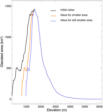
Fig. 11. Area-vs-elevation results, based on summing the hypsometry curves of all glaciers that lie within the Alaskan mascons shown in Figure 1. The black curve shows the observed results for the present day. The orange and blue curves show how we have modified those results to reflect future reductions in the total area of the Alaskan glaciers.
ACKNOWLEDGEMENTS
S. S. is supported by the Regional and Global Climate Modeling Program (RGCM) of the U.S. Department of Energy's, Office of Science (BER), Cooperative Agreement DE-FC02-97ER62402.
Appendix A
- A gl :
-
Ablation rate over glacierized land
- A ugl :
-
Ablation rate over unglacierized land
- c:
-
Constant = 0.03 (Bahr and others, Reference Bahr, Meier and Peckham1997)
- C gl :
-
Accumulation rate over glacierized land
- C ugl :
-
Accumulation rate over unglacierized land
- DDF:
-
Degree-day factor
- d prec :
-
Precipitation gradient
- γ:
-
Constant = 1.36 (Bahr and others, Reference Bahr, Meier and Peckham1997)
- K 0:
-
ERAI Snowfall correction factor
- lr:
-
Environmental lapse rate
- M:
-
Total mass at time t
- M gl :
-
Total glacier mass at time t assuming glacier area changes in response to volume
- M ugl :
-
Total non-glacier mass at time t
- M 0:
-
Total mass at time 0
- $M_{gl}^0 $
:
$M_{gl}^0 $
: -
Total glacier mass at time 0
-
$M_{ugl}^0 $
:
-
Total non-glacier (snow) mass at time t
-
$M_{gl}^1 $
:
-
Total glacier mass under the assumption glacier area is constant
- S gl :
-
Total glacierized area within all mascons
- S ugl :
-
Total unglacierized area within all mascons
- S i :
-
Area of individual glacier
-
$S_i^0 $
:
-
Initial area of individual glacier
-
$S_{gl}^0 $
:
-
Initial area of all glaciers
- Snow SF:
-
adjusted to specific elevation using lr
- SF (t):
-
ERAI snowfall rate
- T (t):
-
ERAI surface temperature
- T 0:
-
ERAI temperature threshold at which precipitation is considered snow
- Temp T:
-
adjusted to specific elevation using lr
- V gl :
-
Total regional glacier volume
- z:
-
Elevation
- ΔV gl :
-
Change in total regional glacier volume
- V i :
-
Volume of individual glacier
- ΔV i :
-
Change in volume of individual glacier
-
$V_i^{\rm 0} $
:
-
Initial volume of individual glacier
-
$V_{gl}^0 $
:
-
Initial volume of all glaciers
- ρ ice :
-
Density of ice


Appendix B FEEDBACK FROM THE CHANGING GLACIER AREA
Here, we describe how we compute the change in glacier area caused by a change in glacier mass, and then how we incorporate that change in area back into our prediction of future changes in total glacier mass. We first note that other methods such as using volume/length scaling (Bahr and others, Reference Bahr, Meier and Peckham1997; Radić and others, Reference Radić, Hock and Oerlemans2008) require information on glacier geometries that we cannot easily incorporate here. Instead, let M gl (t), V gl (t) and S gl (t) be the total mass, volume and area, respectively, of all the Alaskan glaciers, as functions of time. We define the relation between mass and volume as,
 $${V_{gl}} = \displaystyle{{{M_{gl}}(t)} \over {{\rho _{ice}}}}$$
where ρ ice = 917 kg m−3 is the density of ice. We employ a commonly used volume/area scaling relation, (Bahr and others, Reference Bahr, Meier and Peckham1997, Reference Bahr, Pfeffer and Kaser2015) between the volume of an individual glacier and its area:
 $${V_i}\;(t) = c{S_i}\;{(t)^\gamma} $$
where V i (t) (km3) and S i (t) (km2) are the volume and area of a given glacier, which we denote by the subscript i; and c and γ are constants. Bahr and others (Reference Bahr, Meier and Peckham1997) show that Eqn (B2), together with the value γ = 1.36, is a general relation that can be expected to remain valid as glacier areas and volumes change. The relation does not hold for individual glaciers but is effective when applied over large samples of glaciers as implemented below. The parameter c is typically found to be of the order of 0.03. We can invert Eqn (B2) to get:
 $${S_i}(t) = {\left( {\displaystyle{{{V_i}\;(t)} \over c}} \right)^{1/\gamma}} $$
Alaska has ~27 000 glaciers (Kienholz and others, Reference Kienholz2015), which we define as N glaciers, so that i = 1,… N. The total area of all Alaskan glaciers is then:
 $$\eqalign{{S_{gl}}(t)& = \mathop \sum \limits_{i = 1}^N {S_i}(t) = \mathop \sum \limits_i {\left( {\displaystyle{{{V_i}(t)} \over c}} \right)^{1/\gamma}} \cr & = \mathop \sum \limits_i {\left( {\displaystyle{{V_i^0 + {\rm \Delta} {V_i}(t)} \over c}} \right)^{1/\gamma}} }$$
where $V_i^0 $
is the initial (i.e. at time t = 0) volume of an individual glacier, and ΔV
i
(t) is the change in volume. The result (B4) implies that the initial area,
$V_i^0 $
is the initial (i.e. at time t = 0) volume of an individual glacier, and ΔV
i
(t) is the change in volume. The result (B4) implies that the initial area, $S_{gl}^0 $
, is given by:
$S_{gl}^0 $
, is given by:
 $$S_{gl}^0 = \mathop \sum \limits_i {\left( {\displaystyle{{V_i^0} \over c}} \right)^{1/\gamma}} $$
Equation (B4) could be used to find the total glaciated area at any time, but would require knowledge of the original volume. While this could be estimated by Eqn (B2), uncertainties could be large. Instead we make the assumption that the relative change in the volume of each glacier is the same as the relative change in the total glaciated volume:
 $$\displaystyle{{{\rm \Delta} {V_i}(t)} \over {V_i^0}} = \displaystyle{{{\rm \Delta} {V_{gl}}(t)} \over {V_{gl}^0}} $$
where $V_{gl}^0 $
and ΔV
gl
(t) are respectively, the original total volume and change in total volume of all the glaciers. This assumption will not be strictly true, since as the climate warms, glaciers at low elevation will lose volume faster than those at high elevation. Putting (B6) into (B4) gives:
$V_{gl}^0 $
and ΔV
gl
(t) are respectively, the original total volume and change in total volume of all the glaciers. This assumption will not be strictly true, since as the climate warms, glaciers at low elevation will lose volume faster than those at high elevation. Putting (B6) into (B4) gives:
 $$\eqalign{{S_{gl}}(t) & = \mathop \sum \limits_i {\left( {\displaystyle{{V_i^0 + V_i^0 \left( {{{{\rm \Delta} {V_{gl}}(t)} / {V_{gl}^0}}} \right)} \over c}} \right)^{1/\gamma}} \cr & = {\left( {1 + \displaystyle{{{\rm \Delta} {V_{gl}}(t)} \over {V_{gl}^0}}} \right)^{1/\gamma}} \mathop \sum \limits_i {\left( {\displaystyle{{V_i^0} \over c}} \right)^{1/\gamma}} \cr & = {\left( {1 + \displaystyle{{{\rm \Delta} {V_{gl}}(t)} \over {V_{gl}^0}}} \right)^{1/\gamma}} S_{gl}^0 }$$
where the last equality follows from, Eqn (B5).
Equation (B7) is a relation between the new and original total glaciated areas, which requires knowledge only of the original total glaciated volume and the change in total volume. We estimate the change in volume using Eqns (8) and (B1). For the original total volume we use the result $V_{gl}^0 = 1.6 \times {10^4}\;{\rm k}{{\rm m}^{\rm 3}}$
, from Grinsted (Reference Grinsted2013). Grinsted used estimates of the areas of all Alaskan glaciers, converted them to individual glacier volumes using Eqn (B2), and summed over all glaciers to get the total glacier volume. (We obtain this same numerical result by combining Eqn (B2) with the integrated area of our hypsometry.)
$V_{gl}^0 = 1.6 \times {10^4}\;{\rm k}{{\rm m}^{\rm 3}}$
, from Grinsted (Reference Grinsted2013). Grinsted used estimates of the areas of all Alaskan glaciers, converted them to individual glacier volumes using Eqn (B2), and summed over all glaciers to get the total glacier volume. (We obtain this same numerical result by combining Eqn (B2) with the integrated area of our hypsometry.)
The result, Eqn (B7), can be used to update S gl (t) at every time step, from knowledge of the change in glacier volume, ΔV gl (t). Those updated values for the area can be used in Eqns (3) and (5), which are then used in Eqn (8) to find the change in volume. This is then used in (B7) to find S gl (t) for the next time step; etc. We have found, though, a way to combine all these equations (i.e. (B7), (3), (5) and (8)) into a single differential equation; which, when solved, provides an alternative method for computing the change in mass; one that is easier to implement.
We begin by taking the time derivative of Eqn (8), combined with Eqns (3) and (5), to get:
 $$\eqalign{\displaystyle{{{\rm d}{M_{gl}}(t)} \over {{\rm d}t}} = & {C_{gl}} - {A_{gl}}(t) \cr = & \left[ {{K_0}{\rm SF}(t) - \left\{ {\matrix{ 0 & {{\rm if}\quad T(t) \lt {T_0}} \cr {{\rm DDF}(T(t) - {T_0})} & {{\rm if}\quad T(t) \gt {T_0}} \cr}} \right\}} \right]\cr& \times {S_{gl}}(t) \cr = & P(t){S_{gl}}(t)} $$
where P(t) is defined as the quantity inside the large brackets in the second line. Noting that ΔV
gl
(t) and $V_{gl}^0 $
can be related to the change in total mass and the initial total mass, dM
gl
(t)/dt and
$V_{gl}^0 $
can be related to the change in total mass and the initial total mass, dM
gl
(t)/dt and $M_{gl}^0 $
using Eqn (B1), Eqn (B7) becomes
$M_{gl}^0 $
using Eqn (B1), Eqn (B7) becomes
 $${S_{gl}}(t) = {\left( {1 + \displaystyle{{\Delta {M_{gl}}(t)} \over {M_{gl}^0}}} \right)^{1/\gamma}} S_{gl}^0 = {\left( {\displaystyle{{{M_{gl}}(t)} \over {M_{gl}^0}}} \right)^{1/\gamma}} S_{gl}^0 $$
If Eqn (B9) is used to relate A gl (t) to Mass gl (t), Eqn (B8) becomes
 $$\displaystyle{{{\rm d}{M_{gl}}(t)} \over {{\rm d}t}} = P(t){\left( {\displaystyle{{{M_{gl}}(t)} \over {M_{gl}^0}}} \right)^{1/\gamma}} S_{gl}^0 $$
Or, equivalently:
 $${\left( {\displaystyle{{M_{gl}^0} \over {{M_{gl}}(t)}}} \right)^{1/\gamma}} \displaystyle{{{\rm d}{M_{gl}}(t)} \over {{\rm d}t}} = P(T)\; S_{gl}^0 $$
Integrating Eqn (B11) over time between t = 0 and t = t gives:
 $${M_{gl}}(t) = M_{gl}^0 {\left[ {1 + \left( {1 - \displaystyle{1 \over \gamma}} \right)\displaystyle{{S_{gl}^0} \over {M_{gl}^0}} \int_0^t {P(t){\rm d}t}} \right]^{\gamma /(\gamma - 1)}}$$
Suppose we predict the change in mass without taking into account the fact that the glacier area changes as the glacier mass changes. That is what we did when deriving the results shown by the blue curve in Figure 6. We refer to those predictions as $M_{gl}^1 (t)$
. From (B8),
$M_{gl}^1 (t)$
. From (B8), $M_{gl}^1 (t)$
is the solution of:
$M_{gl}^1 (t)$
is the solution of:
 $$\displaystyle{{{\rm d}M_{gl}^1 (t)} \over {{\rm d}t}} = P(t)S_{gl}^0 $$
so that
 $$M_{gl}^1 (t) = M_{gl}^0 + S_{gl}^0 \int_0^t {P(t){\rm d}t}. $$
Then, (B12) can be written as:
 $${M_{gl}}(t) = M_{gl}^0 {\left[ {1 + \left( {1 - \displaystyle{1 \over \gamma}} \right)\displaystyle{{M_{gl}^1 (t) - M_{gl}^0} \over {M_{gl}^0}}} \right]^{\gamma /(\gamma - 1)}}$$
If we denote the change in mass as ${\rm \Delta} M_{gl}^1 (t) = M_{gl}^1 (t) - M_{gl}^0 $
when we do not include the change in area in the computations, and as
${\rm \Delta} M_{gl}^1 (t) = M_{gl}^1 (t) - M_{gl}^0 $
when we do not include the change in area in the computations, and as ${\rm \Delta} {M_{gl}}(t) = {M_{gl}}(t) - M_{gl}^0 $
when we do include the change in area, then (B15) becomes:
${\rm \Delta} {M_{gl}}(t) = {M_{gl}}(t) - M_{gl}^0 $
when we do include the change in area, then (B15) becomes:
 $${\rm \Delta} {M_{gl}}(t) = M_{gl}^0 \left( {{{\left[ {1 + \left( {1 - \displaystyle{1 \over \gamma}} \right)\displaystyle{{{\rm \Delta} M_{gl}^1 (t)} \over {M_{gl}^0}}} \right]}^{\gamma /(\gamma - 1)}} - 1} \right)$$
and using γ = 1.36,
 $${\rm \Delta} {M_{gl}}(t) = M_{gl}^0 \left( {{{\left[ {1 + 0.264\displaystyle{{{\rm \Delta} M_{gl}^1 (t)} \over {M_{gl}^0}}} \right]}^{3.78}} - 1} \right)$$
For $Mass_{gl}^0 $
we use Grinsted's (Reference Grinsted2013) value:
$Mass_{gl}^0 $
we use Grinsted's (Reference Grinsted2013) value:
 $$\eqalign{Mass_{gl}^0 & = V_{gl}^0 \times {\rho _{ice}} = 1.6 \times {10^4}\;{\rm k}{{\rm m}^3} \times 917\;{\rm kg}\;{{\rm m}^{ - 3}}\cr & = 1.5 \times {10^4}\;{\rm Gt}}$$
Our method, then, includes the effects of a changing area on the mass estimates and proceeds as follows. First, we use Eqns (3)–(8) to find the change in glacier mass when the area feedback is not included. That change is denoted here as ${\rm d}M_{gl}^1 (t)/{\rm d}t$
, and results are shown by the blue curve in Figure 6. We then use Eqn (B17) (together with the value of
${\rm d}M_{gl}^1 (t)/{\rm d}t$
, and results are shown by the blue curve in Figure 6. We then use Eqn (B17) (together with the value of $M_{gl}^0 $
gven in Eqn (B18)), to find the change in mass, dM
gl
(t)/dt, after the area feedback has been included.
$M_{gl}^0 $
gven in Eqn (B18)), to find the change in mass, dM
gl
(t)/dt, after the area feedback has been included.
Appendix C FEEDBACK FROM CHANGING GLACIER GEOMETRY
Our general approach for estimating the impact of the changing mass on K
0 and T
0 is listed: (1) We use Eqn (B9), together with the value of $M_{gl}^0 $
.given in Eqn (B18), to update the total glacier area at each time step. In general, the area decreases with time as the total mass decreases with time. (2) We distribute that area loss over different elevation bands, preferentially taking mass away from the lower elevations using two different methods (discussed below). This causes the average glacier elevation to increase with time. (3) We quantify the average elevation increase at each time step. (4) We use estimates of the lapse rate, lr, and the precipitation gradient, d
prec
, to estimate the change in K
0 and T
0 at each time step (notation taken from Radić and Hock, Reference Radić and Hock2011) using the change in average elevation. Our method of updating the total glacier area, (1), has already been described in Appendix B. Here, we describe the remaining three steps, (2)–(4), in detail.
$M_{gl}^0 $
.given in Eqn (B18), to update the total glacier area at each time step. In general, the area decreases with time as the total mass decreases with time. (2) We distribute that area loss over different elevation bands, preferentially taking mass away from the lower elevations using two different methods (discussed below). This causes the average glacier elevation to increase with time. (3) We quantify the average elevation increase at each time step. (4) We use estimates of the lapse rate, lr, and the precipitation gradient, d
prec
, to estimate the change in K
0 and T
0 at each time step (notation taken from Radić and Hock, Reference Radić and Hock2011) using the change in average elevation. Our method of updating the total glacier area, (1), has already been described in Appendix B. Here, we describe the remaining three steps, (2)–(4), in detail.
For step (2), we use hypsometry (area-vs-elevation) data for every Alaskan glacier (Larsen and others, Reference Larsen2015), and sum them over all glaciers lying within the glacier mascons shown in Figure 1 to obtain an estimate of the total glaciated area lying in each 30 m elevation band. This total area-vs-elevation field is shown as the black curve in Figure 11. The glaciers' elevation distribution increases from sea level up to an elevation of 1575 m, then decreases. The total glacier area, integrated over all elevations, is 7.4 km × 104 km. We assume these values describe the present-day area-vs-elevation field.

Fig. 12. Area-vs-elevation results, based on the present-day hypsometry results. The black curve (the same as the black curve in Fig. 11) shows the present-day results. The orange and blue curves illustrate two methods we have used to modify those results to reflect future reductions in total area. For the orange curve (the same as the orange curve in Fig. 11) we have compressed the original curve at low elevations. For the blue curve we have truncated the original curve to remove low elevations. Both the orange and blue curves reflect the same total glaciated area.
At a later time, the total glacier area will have decreased. While the geometry adjustments in reality are complex (Harrison, Reference Harrison2013) and will be unique to each glacier, we chose a simpler more generalized approach here. We assume this decrease occurs mostly at lower elevations. We use two ad hoc methods for distributing this decrease over elevation. For our default method, we assume the new area-vs-elevation field is identical to the original field for elevations >1575 m. For elevations <1575 m, we compress the area-vs-elevation field as shown by the orange and blue curves in Figure 11 (corresponding to total areas of 5.7 km × 104 km and 4.9 km × 104 km, respectively: approximately the total glacier areas we predict for the years 2080 and 2100). Each of those compressed fields has the same general shape as the original field, but has been squeezed in from the lower elevations, so that all elevations <1575 m have lost glacier area, and the lowest elevations are missing glaciers entirely. We refer to this as the compression method.
For our second method, which we refer to as the truncation method, we start at the lowest elevation, and remove all glaciers as the elevation increases, until the total remaining area equals the desired, decreased area. Figure B2 shows what the resulting area-vs-elevation curves look like for these two methods. We use results computed using the truncation method only to help assess the uncertainties in our final mass loss results.
For step (3), we formulate a method of using an area-vs-elevation field to find the average glacier elevation, and we use the three area-vs-elevation fields shown in Figure 11 to estimate how that characteristic elevation changes as the total glacier area changes. For each area-vs-elevation field, we generate a simulated glacier mass time series as follows. We start with the 2003–2014 ERAI time series of temperature and snowfall rate, averaged over all the Alaskan glacier mascons; the same T (t) and SF (t) time series described in Section 3 above. The average elevation of the Alaskan glacier mascons is 1008 m, so we assume those values of T (t) and SF (t) describe the temperature and snowfall rate at that elevation. We then assign a temperature and snowfall rate to each elevation band in the area-vs-elevation field. We do this by assuming values for the lapse rate, lr and the precipitation gradient, d prec . Specifically, for the band at an elevation of Elev, we assume that the temperature is
 $$Temp(t,z) = T(t) + lr \times (z - 1008\;{\rm m})$$
and that the snowfall rate is
 $$Snow(t,z) = {\rm SF(}t{\rm )} \times [1 + {d_{\,prec}} \times (z - 1008\;{\rm m})]$$
To find the total snowfall rate over the entire glaciated area, we multiply Snow(t, z) by the area in the z elevation band, and sum over all the z bands. To find the total melting rate over the entire glaciated area, we assume the melting rate is
 $$\left\{ {\matrix{ 0 & {{\rm if}\quad Temp(t,z) \lt 0{\rm ^\circ} {\rm C}} \cr {{\rm DDF[}Temp(t,z) - 0{\rm ^\circ} {\rm C]}} & {{\rm if}\quad Temp(t,z) \gt 0{\rm ^\circ} {\rm C}} \cr}} \right\}$$
We then multiply by the area in the z band and sum over all the z bands. We use the value DDF = 2.3 mm °C−1 d−1, obtained above Eqn (10) by fitting to GRACE data. To get the total mass, we integrate the total snowfall rate minus the total melt rate over time, as done in Eqn (8) for the ERAI fields. This gives us a simulated total glacier mass time series for 2003–2014.
We then fit a single characteristic elevation to that time series. The elevation fitting is actually done by fitting K 0 and T 0 to the time series, but relating those parameters to the elevation through the lapse rate and the precipitation gradient. Specifically, if elevation is the parameter we are fitting to the simulated data, then we assume that K 0 = 1 d prec (z − 1008 m) and T 0 = 0°C − lr (z − 1008 m). Note that to obtain T 0, we subtract lr (z − 1008 m) from 0°C, rather than add it.
We apply this method of finding the average elevation to each of the three area-vs-elevation fields shown in Figure 11: one corresponding to the total glacier area at the present time, and two corresponding to total glacier areas at future times. We find that the characteristic elevations vary nearly linearly with the total glacier area; a conclusion that appears to hold no matter what values we assume for lr and d prec . We fit a line to those three values (of average elevation vs total glacier area), and use the slope along with the lr and d prec values to estimate the linear dependence of glacier elevation on total glacier area.
For step (4), we adopt values for lr and d prec . At each time step we compute the total glacier area, as described by (B9), and we use our step (3) estimate of the linear dependence of characteristic glacier elevation on total glacier area for those values of lr and d prec , to estimate a characteristic elevation of the glaciers (Figure 12). We then use those same values of lr and d prec to extrapolate the GRACE-derived values of T 0 and K 0 up to the inferred characteristic glacier elevation. We use those values in Eqns (3), (5) and (8), to predict the future mass loss.


 Open access