

INTRODUCTION
Development of agricultural technology, in terms of new seeds/crop genotypes and cultivation practices, results from experiments conducted at research stations where the biophysical environments are generally homogeneous. However, the developed technology is targeted for much larger environments, i.e. farmers’ fields, characterized by large soil heterogeneity and variation in land preparation, poorly performing crop production methods and poor protection methods. Therefore, performance of the new technology or recommended crop production package must be evaluated in farmers’ fields, and such experiments are referred as on-farm trials.
Riley and Alexander (Reference Riley and Alexander1997) have given an overview of statistical literature on on-farm research and Fielding and Riley (Reference Fielding and Riley1998) have discussed experimental designs for on-farm fertilizer trials. The present study focuses on the on-farm evaluation of improved varieties of legumes chickpea (Cicer arietinum) and mung bean (Vigna radiata) in comparison to the local varieties and practices in Afghanistan. Legumes are very important to meet the dietary requirement in many countries, including Afghanistan, particularly to their poor population. Legumes provide nutrition and health security as they contain substantial proportion of macro and micronutrients (Ca, P, K, Fe, Zn), vitamins (niacin, vitamin-A, ascorbic acid, inositol), fibre and carbohydrates for balanced nutrition and lower cholesterol levels. A survey report (National Nutrition Survey Afghanistan, 2013) presents the nutritional status of the population in Afghanistan and more than half of children under the age of five are malnourished (WFP - http://www.wfp.org/node/3191). In rotation with cereals, legumes form the soil nutritional arm of the sustainable cropping systems. The low productivity of locally grown legumes in farmer conditions falls too short to meet the growing human population need in Afghanistan. Therefore in order to enhance adoption of improved food legumes by farmers, the International Centre for Agricultural Research in the Dry Areas (ICARDA), and Ministry of Agriculture, Irrigation and Livestock (MAIL) initiated the demonstration trials with a few improved varieties of chickpea and mung bean starting June 2009 in three provinces of Afghanistan (ICARDA, 2014).
Statistical analysis of data from the on-farm trials is normally based on the estimation and comparison of means using two-sample t-test, paired t-test or analysis of variance (Mead et al., Reference Mead, Curnow and Hasted2002; Snedecor and Cochran, Reference Snedecor and Cochran1989). However, an approach based on stochastic dominance of the improved varieties appears more appropriate in the context of on-farm trials when the farmer has to make his decision on preference of a crop production package/technology. Anderson (Reference Anderson1974) soundly argued that the approach of a farmer would be to remain risk averse, particularly in the presence of so many adversely affecting and uncontrolled factors of crop production, such as biotic and abiotic stress factors. Since then such a stochastic dominance approach has been exploited in several studies, including Haddad et al. (Reference Haddad, Singh and Mamdouh2005) on rainfed barley in Jordan. Experimental designs used in Haddad et al. (Reference Haddad, Singh and Mamdouh2005) were suitable to compare the best-bet-package (recommended technology) with the farmer's package from the perspectives of the farmer and the state as paired datasets were available on each farm under both types of packages. The comparisons were carried out using means and risks to meet a given target based on empirical and fitted, normal and non-normal distribution functions. Similar approaches based on cumulative frequencies of the empirical and modelled distributions have been discussed by Vanlauwe et al. (Reference Vanlauwe, Coe and Giller2016) on maize in Western Kenya and beans in Eastern Rwanda and Coe et al. (Reference Coe, Njoloma and Sinclair2016) on maize in Malawi.
As a part of out-scaling research, on-farm trials are routinely conducted to demonstrate the performance of new production packages and summarized in terms of mean, standard deviation and precision. Such information generated from similar on-farm trials already conducted could be used to strengthen and widen the scope of statistical inference that can be drawn from the current on-farm trial data. The frequentist approach (FA) for analysis of data is based on the notion that there is only a single value of the parameter of interest, which is an extremely narrow window chosen to view the wide sky of the parameter space, and is normally derived from likelihood of the data. But in absence of a priori information about the parameter space, FA is the natural choice. The FA does not make use of the prior information while Bayesian approach (BA) does. BA has been a part of standard texts in statistics (Carlin and Louis, Reference Carlin and Louis2009; Gelman et al., Reference Gelman, Carlin, Stern, Dunson, Vehtari and Rubin2013).
While BA has found its application in evaluating crop variety trials in single or multi-environments (Crossa et al., Reference Crossa, Perez-Elizalde, Jarquin, Cotes, Viele, Liu and Cornelius2011; Edwards and Jannink, Reference Edwards and Jannink2006; Forkman and Piepho, Reference Forkman and Piepho2013; Josse et al., Reference Josse, van Eeuwijk, Piepho and Denis2014; Omer et al., Reference Omer, Abdalla, Mohammed and Singh2015; Singh et al., Reference Singh, Al-Yassin and Omer2015), its application in context of analysis of data from on-farm trials has been limited. While the recommended improved practices could be included in the model with their effects treated as fixed (i.e. constants), the farmer practice varies with the farm or the farmer. In the latter case, the farmer practice effects may be assumed as random. In this situation, one compares an estimate of a single mean for the recommended practice with mean of various practices chosen by the farmers in a given environment. Furthermore, while the recommended package is kept constant over a number of environments (districts), the group of farmers and their practices vary within a location, hence their means also may vary with environment. In an Afghanistan-ICARDA project, BA appeared more appropriate to weigh in the information from the trials in the past. Given the data from few earlier years on-farm trials in broadly similar biophysical environment, the objective of this study is to present a BA for analysis of on-farm trials data and apply the method and computing codes for analysis of chickpea and mung bean trials in Afghanistan in 2012 with prior information extracted from 2009 to 2011 data. Mean productivity of the improved varieties has been estimated as well as the probability that the variety under evaluation exceeds the set target level. We also compared the results under BA with that under the FA, the line of approach normally one takes by default.
MATERIALS AND METHODS
On-farm trials datasets
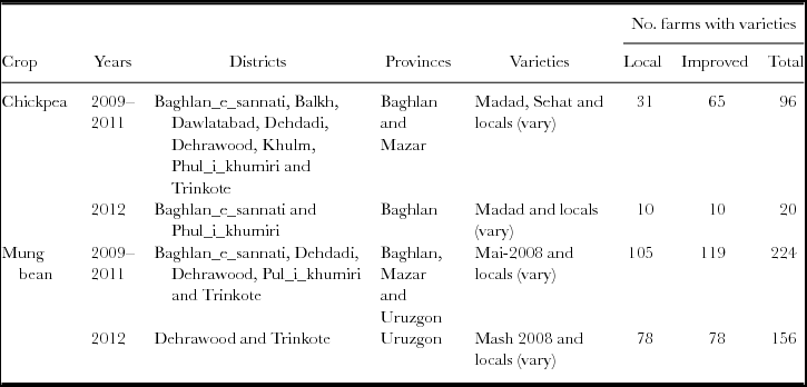
This study used datasets generated under Afghanistan project (CLAP, Sub-component 2.3: Improved Food, Fodder and Vegetable Crops, IFVEC) from farmer participatory demonstration trials in eight districts of Baghlan, Mazar and Uruzgan provinces during 2009–2012 (Table 1). These datasets have been used in ICARDA (2014) and Alokozai et al. (Reference Alokozai, Rasoli, Safi, Manan, Rizvi, Tavva, Singh and Saharawat2016). Farmers’ participatory demonstrations were laid out in order to popularize improved varieties of chickpea (Sehat and Madad) and mung bean (Mai-2008 and Mash 2008) along with their associated best practices. Each demonstration was laid out in an area of 1000 m2. Besides the use of improved varieties of crops, best agronomic practices such as the use of seed rate (100 and 50 kg per ha for chickpea and mungbean, respectively), optimum fertilizer (50 kg urea and 100 kg diammonium phosphate (DAP) for chickpea and 50 kg urea and 120 kg DAP for mungbean per ha) and applying weed control methods were included in the demonstrations. The yields obtained in the demonstrations were compared with the yields obtained by farmers growing local varieties with local agronomic practices. The datasets for 2012 were evaluated to compare the packages for productivity and risk, while the data from 2009 to 2011 were used for prior information on the variance parameters in the Bayesian analysis.
Table 1. Number of farms with improved varieties and recommended packages and the local varieties, 2009–2012, selected provinces in Afghanistan.
Statistical models
Models: Let yrij be yield under the recommended package of technology, denoted by subscript r, given to farmer j in village or district or environment i, where j = 1. . .ni, i = 1. . .p; ni is the number of farmers using the recommended practice and p is the number of locations or environments (location–year combinations). As was the case, not all the recommended practices were taken by the same farmer. The statistical model used to describe the data yrij is assumed as:
 $$\begin{equation}
{y_{rij}}\, = \mu + {\mu _{ri}}\, + \,{\varepsilon _{ij}},
\end{equation}$$
$$\begin{equation}
{y_{rij}}\, = \mu + {\mu _{ri}}\, + \,{\varepsilon _{ij}},
\end{equation}$$
where μ is general mean for all the plots under recommended and farmer practices, μri is effect of the recommended package when grown in i-th environment and is assumed as fixed. In case of more than one recommended package, one may introduce an additive model with effects of the environment and recommended package. Furthermore, if the environment comprises multi-location and multi-year scenario, it is more appropriate to introduce a random year effect within location as an additional component in the above equation. The random errors εij are assumed to follow N(0, σ2r). σ2r is variance between farms under a recommended package in an environment and is assumed constant over the environment.
In case of modelling the yield under farmer practice, we may take into account the fact that farmer practices vary within as well as between the environments. Let y 0ik be the yield in farmer k field under his practice, denoted by subscript 0, in environment i(k = 1. . .ni, i = 1. . .q), where q is the number environments under farmers practices. The model assumed on the above line would be
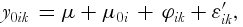 $$\begin{equation}
{y_{0ik}}\, = \mu + {\mu _{0i}}\, + \,{\varphi _{ik}} + {\varepsilon '_{ik}},
\end{equation}$$
$$\begin{equation}
{y_{0ik}}\, = \mu + {\mu _{0i}}\, + \,{\varphi _{ik}} + {\varepsilon '_{ik}},
\end{equation}$$
which differs from the model for recommended package in the sense that the farmer practice effect φik, over the environment under farmers practices μ0i, varies with the farmer (k) within environment i and can be assumed as N(0, σ2fw). It may be expected that the variance due to the term (φik + ε'ik) will not be lower than σ2r while it is possible that the scale of response in the farmer practices plots could be substantially low, resulting in a lower variance for φik + ε'ik. In this situation, the variance parameter σ2fw cannot be separated from variance of ε'ik, therefore, we take σ2fw = Var(φik + ε'ik). Furthermore, μ0i varies not only with the environment (i) but because the group of farmers also vary with the environment (i). One way to filter the effect of farmer practice in an environment i would be to remove the effect of the environment based on the recommended practices, i.e., the difference δi = μ0i − μri will comprise of the net farmer effects in the environment i and δi is assumed to follow N(0, σ2fb), where σ2fb is variance between environment means for the net farmer practice responses. Thus the model (2) can be re-written as follows:
 $$\begin{equation}
{y_{0ik}}\, = \mu + {\mu _{ri}}\, + {\delta _i} + \,{\varphi _{ik}} + {\varepsilon '_{ik}}.
\end{equation}$$
$$\begin{equation}
{y_{0ik}}\, = \mu + {\mu _{ri}}\, + {\delta _i} + \,{\varphi _{ik}} + {\varepsilon '_{ik}}.
\end{equation}$$
Estimates of variance parameters σ2r and σ2fw can be obtained as sample variances of responses from each environment. The σ2fb can be estimated by sampling variance of  ${\bar{y}_{0i}}\, - {\bar{y}_{.i}}$, i = 1. . .q, where ${\bar{y}_{0i}}$ and ${\bar{y}_{.i}}\,$ are observed means for environment i, respectively, under farmer practice and recommended practice(s) common over all the environments. The estimates of means μri and μ0i were obtained as respective sample means along with their sampling standard errors of means. The formulae are available in standard text (Mead et al., Reference Mead, Curnow and Hasted2002; Snedecor and Cochran, Reference Snedecor and Cochran1989). In case of data obtained from more than one recommended practice and blocking factors, one may use a linear model or mixed model to obtain the residual variance for each environment. The above approach is FA.
Bayesian approach
We describe BA in brief here to infer a single parameter θ using data represented as the vector y = (y 1,. . ., yn)'. Let the probability distribution or the likelihood of observing y based on a value of θ be denoted by f ( y | θ). Furthermore, let the prior information on θ be described in terms of its probability distribution function say g(θ), called an a priori distribution of θ, or simply a prior for θ. This distribution may arise from a series of already observed datasets and may serve as a degree of belief in θ. For instance, one may obtain distribution of mean or variance of productivity from a series of on-farm trials conducted in past. The Bayesian inference on θ is drawn as the conditional probability distribution of θ given the current data y or its summaries. Following Bayes’ theorem, the conditional probability distribution can be expressed as f(θ | y) ∝ g (θ)f(y/θ) and is called the a posteriori or simply a posterior density function of θ and is an integration of prior information (g(θ)) with the likelihood (f (y |θ)) of the current data and thus differs from the FA. The above analogy can be extended to the case of more than one parameter. Statistical inference under BA is drawn as conditional means, credible interval and probability statements on the parameters of interest given the data.
The BA was applied using WinBUGS software (Spiegelhalter et al., Reference Spiegelhalter, Thomas, Best and Lunn2003) and R-codes (R Development Core Team, 2009). Models parameters whose prior distributions were used in the analysis were: σ2r, σ2fw and δi (for all the environments i). For the simulations, the number of iterations was set at 500,000 number of simulations on which the posterior distribution was summarized at 10,000 and the number of chains at three.
A priori distributions and selection of the better prior
The prior distribution of these parameters were obtained from analysis of data on similar on-farm trials during 2009–2011, which presents the values of sample standard deviations (SSD) to estimate σr and σfw, as well as estimates of δi for data range during 2009–2011. The distributions of the estimators (sampling variances) were examined as in the following. Singh et al. (Reference Singh, Al-Yassin and Omer2015) in the context of a series of barley trials explored the distribution of standard deviation components (SDC) instead of variance components (SDC2) and found that SDCs are closely normally distributed and are in obvious positive range. In the present case, we fitted the normal distribution and also log-normal distribution to the SSD used for estimating σr and σfw, and their skewness and kurtosis were insignificant at 5% level of significant.
The yield values and standard deviation (or the variance) components were positive, so their distributions were constrained to the positive values of normal distributions. Thus, the constrained distribution for σr can be denoted by σr ~ N(a, b)+, where a and b are mean and variance of the normal distribution. Instead of variance, one uses precision parameter τ = b −1 (inverse of variance) in the Bayesian context and the above distribution following the WinBUGS code, is expressed as σr ~ dnorm(a, τ)*I(0,), where I(0,) restricts the generated values of σr ~ N(a, b) in the positive range. If a random variable, X ~ N(a, b) then eX, always positive, follows log-normal distribution and is expressed as ~ LN(a, b). The priors are presented in Table 2 along with the resulting values of the discrepancy statistics. Of the two sets of priors, the better of the two models was selected on the basis of deviance information criterion (DIC), lower the better (also in Table 2). Although there are small differences in the DIC values of these two priors, the set of chosen priors based on positive normal distribution for SSD (Prior set 1) is better for chickpea and that based on log-normal distribution is better for mung bean (Prior set 2). The Monte Carlo errors were acceptably small. The essential codes for the models are given in Supplementary Appendix S1 (available online at https://doi.org/10.1017/S0014479717000187).
Table 2. Sets of a priori distributions of various parameters used in analysis and discrepancy statistics DIC.
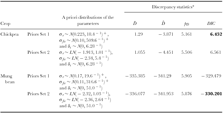
*  $\bar{D}$ = the a posteriori mean of (–2 × log-likelihood). $\hat{D}$ = –2 × log-likelihood at the a posteriori means of parameters. pD = effective number of parameters. DIC = Deviance information criterion, smaller DIC values shown in bold.
RESULTS AND DISCUSSION
For the better of the two sets of priors selected using DIC (Table 2), the posterior means of the parameters of interest were obtained along with their posterior standard deviations (Table 3). The estimates of mean under FA and the posterior mean under the Bayesian were equal (when rounded to 2 decimals) while the standard errors and posterior standard deviations differed in chickpea trials. Posterior standard deviations of chickpea means in both the practices were higher than the corresponding frequentist standard errors. These higher values are arising from the contributions of the a priori information to the various degrees. BA is expected to take into account the distribution of parameters where a priori information is available. The means and limits of 95% credible intervals for the recommended package(s), growing Madad variety of chickpea and Mash 2008 of mung bean, were higher compared to the respective values for the farmer package on average. Using the simulations in the Bayesian analysis, the probability that the recommended package yield is higher than the farmer package was 94.7% and 98.6% for the two districts in chickpea and 100% in case of mung bean. The yield productivity did not show significant difference between the districts for the respective package.
Table 3. Bayesian and frequentist estimates of grain yields for the two legumes in the districts of Afghanistan, 2012.
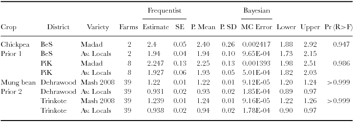
BeS= Baghalan-e-sannati. PiK= Phul-i-khumiri. SE= Standard error. P. Mean= Posteriori mean. P. SD= Posteriori standard deviation. MC Error=Monte Carlo error. Lower, Upper = lower and upper limits of 95% credible interval. Pr (R>F)= Probability of yield exceeding under recommended package compared to farmer practice (Bayesian approach).
Stochastic dominance
Another aspect when comparing the technologies could be the risk involved in achieving a specified yield target, in terms of probability that a technology will yield a specified amount or more. The simulated values, available in the process of computation, were used for comparing means and the probabilities of exceeding a target yield under a package are shown in Figure 1a for a range of target yields. For chickpea production, if a target of 2 Mg/ha is set at Baghlan_e_sannati, chances are over 95% to achieve by growing Madad, while the chances are around a third under the local packages. At Phul-i-khumiri, the chances are further higher under the improved package and further lower under the local. At any given target, chance is higher to achieve with Madad than with the local practice. To achieve a higher target, say 2.5 Mg/ha, there is no possibility under the local package while at Baghlan the chance is around 34% with Madad cultivar. We also notice that there was a crossover in the stochastic dominance of the same packages between the two locations. For instance, to achieve a target higher than 2.12 Mg/ha, Baghlan area is less risky (i.e. more safe in terms of higher probability) compared to the Phul-i-khumiri, while for a target lower than 2.12 Mg/ha, Phul-i-khumiri is relatively less risky. Presence of a crossover makes one technology superior to the other in the range of specific targets. Thus, introduction of an additional dimension along target in the stochastic approach helps examining the relative superiority of each the technology, of course in specific domain, unlike the comparisons based on means where only an overall comparison is possible.
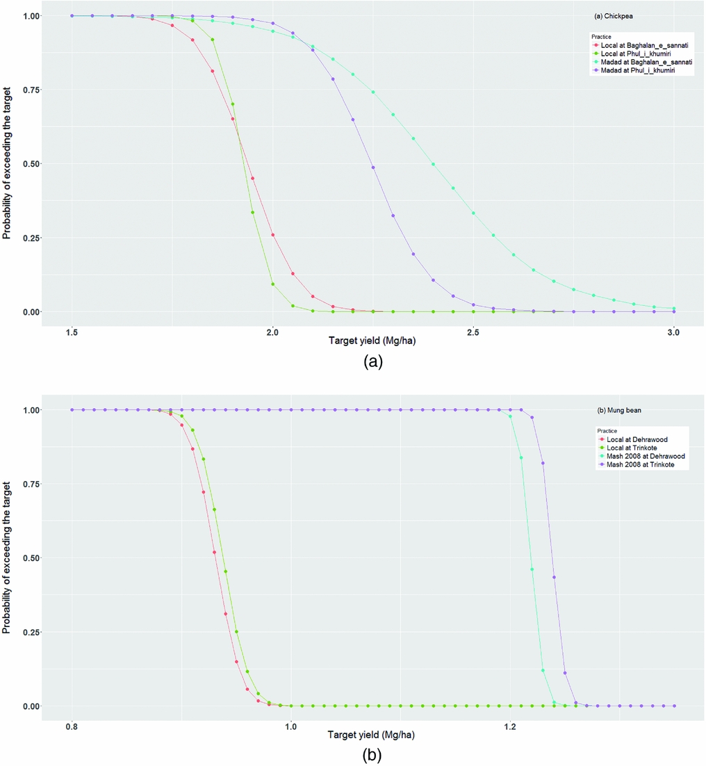
Figure 1. Risk curves for (a) improved chickpea variety Madad and a local one in Baghlan_e_sannati and Phul_i_kumiri districts, and (b) improved mung bean varieties Mash 2008 and a local one in Dehrawood and Trinkoli districts, 2012, Afghanistan.
The trend in mung bean was similar for superiority of the improved cultivar over the local practice, except there was no crossover in the curves unlike the chickpea (Figure 1b). There appears to be no chance of achieving 1 Mg/ha yield under the farmer package, while there is an almost certainty in achieving this level with the improved variety Mash 2008, and the probability of achieving the target of 1.2 Mg/ha exceeds 97%.
BA incorporates the realities of the data generation process more fairly than a frequentist method, in which the parameter(s) are assumed as fixed constants. In a fixed constant approach, one assigns a single value with probability one if translated in the context of random variable. In the on-going process of similar on-farm trials conducted over a range of environments, various parameters such as means and standard deviations (variances) over a number of farms have a series of estimates arising from those environments. The statistical distribution of these estimates helps in providing a measure of belief in the likely parameter values, and thus can be used as a priori distributions. This information in general remains ignored, while analysing any current datasets.
In the context of on-farm trials, this study uses a Bayesian framework. One of the challenges of a BA is to find a reliable or justifiable a priori distribution. The standard estimation procedures, non-Bayesian or FA, when applied on on-farm trials of previously conducted on-farm trials during 2009–2011 in similar agro-ecologies, provided the basis of determining the a priori distributions. The Bayesian estimates of the parameters, calculated and called as posterior means lie between their a priori means and the frequentist estimates (Gelman et al., Reference Gelman, Carlin, Stern, Dunson, Vehtari and Rubin2013; Lindley, Reference Lindley, Godambe and Sprott1971), and thus depend on the prior distributions used. In the present study, we used the priors for the SSD and for the mean arising from the farmer's package. We assumed the environment or district effects as fixed as they differ in the biophysical properties and not many replicates are available for a district to form a justifiable prior distribution. Further, the distributions of SSDs were found to follow positively truncated part of normal distribution (as in Singh et al., Reference Singh, Al-Yassin and Omer2015) and also log-normal distributions. Thus, two sets of priors were considered and the better of the two was taken for analysis of the current (2012) datasets. The two crops supported different distributional forms for the prior parameters.
The concept of stochastic dominance was introduced by Anderson (Reference Anderson1974) and has found recent applications on on-farm trials data analysis using a non-BA (Coe et al., Reference Coe, Njoloma and Sinclair2016; Vanlauwe et al., Reference Vanlauwe, Coe and Giller2016). One of the clear advantages of the stochastic dominance method is the estimation of risks or safety of production for a given target, and this perspective is important for farmers who are risk averse when new technologies are recommended to them. Also depending on the intended target level, one would be able to choose between the technologies whenever the risk curves between technologies cross each other, and one does not get restricted by choice of technology for its overall mean, as highlighted by Vanlauwe et al. (Reference Vanlauwe, Coe and Giller2016).
Effectiveness of a BA arises from suitability of the priors for various parameters included in the model. A limitation of the present study is that the priors’ distributions were obtained from a small number of environments (location–year combinations): 5–8 for various SSDs and 4–5 for the δi’s in equation (3). However, the approach presented can be out-scaled for situations with a larger number of data points for determining the a priori distributions, and thus making the approach more robust. Furthermore, the BA can be generalized to model data from various experimental designs with fixed or random effects expressed as linear or even non-linear models with normal or non-normal errors, along with appropriate a priori distributions of the parameters involved. Experimental designs vary with the objective of the on-farm trials, e.g. to identify factors which determine yield gaps at farmers’ fields, a factorial design with a small number of two-level factors in complete blocks may be used. Assessment of yield gaps using BA would be a worthwhile study in future. Comparing experimental designs using a BA will depend on the objectives of the study. For example, in crop variety trials, estimates of the genotype effects and other parameters such as heritability and genetic gains, and their precision under the BA could be used to compare the experimental designs (Omer et al., Reference Omer, Abdalla, Mohammed and Singh2015; Singh et al., Reference Singh, Al-Yassin and Omer2015).
CONCLUSIONS
Legume on-farm trials are routinely conducted to demonstrate the performance of recommended practices using improved genotypes and practices of chickpea and mung bean in Afghanistan. The process generates so much information but is hardly utilized under the FA of analysis. A BA provides the scope for capturing the a priori information to be used in the analysis of current data. This study demonstrated an application of Bayesian analysis on-farm data, comparing improved and local varieties of chickpea and mung bean in Afghanistan. The BA estimates, called posterior means, as well as risks for various chosen targets were evaluated and the recommended practices were found superior to the local practices in terms of means and risks.
SUPPLEMENTARY MATERIAL
To view supplementary material for this article, please visit http://doi.org/10.1017/S0014479717000187
Acknowledgements
Authors are thankful to anonymous reviewers, a language editor and Dr. Aden Aw-Hassan (ICARDA) for their comments and suggestions, which substantially improved the presentation of the manuscript. Authors are also thankful to International Fund for Agricultural Development (IFAD) for their financial support, and Ministry of Agriculture, Irrigation and Livestock (MAIL) of Afghanistan and ICARDA Provincial teams involved in the field data collection.


 Open access