


Introduction
The Ross Sea is considered to be one of the most productive regions in the Antarctic and is associated with significant uptake of atmospheric carbon dioxide (Arrigo et al. Reference Arrigo, Weiss and Smith1998, Smith et al. Reference Smith, Shields, Peloquin, Catalano, Tozzi, Dinniman and Asper2006). The Ross Sea polynya is created by the northward displacement of sea ice by strong winds blowing off the Ross Ice Shelf. New ice is formed during winter in the polynya leading to the production of dense brine and High Salinity Shelf Water, which can flow off the shelf as part of the global thermohaline circulation (Orsi & Wiederwohl Reference Orsi and Wiederwohl2009).
The timing of phytoplankton blooms in the Ross Sea is strongly dictated by physical factors (ice retreat, solar irradiance and wind mixing). Arrigo et al. (Reference Arrigo, Weiss and Smith1998) and Arrigo & van Dijken (Reference Arrigo and van Dijken2004) reported that the opening of the polynya is dependent on the ice cover compactness and thickness, which is regulated by winter air temperatures rather than by katabatic winds. Once the polynya is open, winds (in conjunction with meltwater input from ice) regulate the onset of the bloom by controlling water column stratification. It has been suggested that strong winds occurring early in the season delay the bloom by reducing water column stability (Arrigo et al. Reference Arrigo, Weiss and Smith1998, Arrigo & van Dijken Reference Arrigo and van Dijken2004).
It has been suggested that as the Ross Sea polynya expands, blooms dominated by Phaeocystis antarctica Karsten occur followed by increased diatom growth (Arrigo et al. Reference Arrigo, Robinson, Worthen, Dunbar, DiTullio, VanWoert and Lizotte1999, Smith et al. Reference Smith, Ainley, Arrigo and Dinniman2014a). However, more recent observations have found variability in this phenology (Arrigo & van Dijken Reference Arrigo and van Dijken2004, Smith et al. Reference Smith, Shields, Peloquin, Catalano, Tozzi, Dinniman and Asper2006), and it has been suggested that their occurrence is dependent upon environmental conditions rather than gradual successional dynamics (Arrigo et al. Reference Arrigo, DiTullio, Dunbar, Robinson, VanWoert, Worthen and Lizotte2000).
Smith et al. (Reference Smith, Asper, Tozzi, Liu and Stammerjohn2011a, Reference Smith, Shields, Dreyer, Peloquin and Asper2011b) described chlorophyll dynamics in the Ross Sea polynya and found that a combination of physical (advection, wind mixing) and biogeochemical (nutrient limitation, zooplankton ingestion and aggregate sinking) factors regulated fluctuations on short period (a few days) and small spatial (tens of kilometres) scales. This results in substantial biological patchiness in the Ross Sea (Hales & Takahashi Reference Hales and Takahashi2004, Smith et al. Reference Smith, Shields, Peloquin, Catalano, Tozzi, Dinniman and Asper2006). Kaufman et al. (Reference Kaufman, Friedrichs, Smith, Queste and Heywood2014) further clarified the magnitude of these spatial and temporal variations and found that the scales of the variability were small enough to be missed by most ship-based surveys.
It is unclear what mechanisms limit and terminate the spring phytoplankton bloom (defined by a rapid increase in phytoplankton biomass inferred from chlorophyll a). During spring, irradiance is the main factor limiting phytoplankton growth (Smith et al. Reference Smith, Shields, Peloquin, Catalano, Tozzi, Dinniman and Asper2006). The termination of the main spring bloom and the limiting factor of subsequent blooms during the summer are probably dependent on another mechanism. Sedwick & DiTullio (Reference Sedwick and DiTullio1997) hypothesized that in high light environments, lower iron concentrations could favour diatom growth over P. antarctica as stratification continues to strengthen during summer. However, to date there are no data to suggest that the iron uptake capabilities of diatoms differ significantly from that of P. antarctica. Indeed, Sedwick et al. (Reference Sedwick, Marsay, Sohst, Aguilar-Islas, Lohan, Long, Arrigo, Dunbar, Saito, Smith and DiTullio2011) found that iron concentrations in spring and summer were similar as a result of rapid early spring removal by Phaeocystis. Smith et al. (Reference Smith, Shields, Dreyer, Peloquin and Asper2011b) suggest that mixing events may contribute to the termination of blooms, at least in certain locations, by vertically redistributing standing stocks. Smith & Asper (Reference Smith and Asper2001) suggested that P. antarctica became iron-limited and sank rapidly from the euphotic zone as aggregates. It is probable that the combination of all of these mechanisms triggers the end of the spring bloom, while changes in iron availability alter phytoplankton composition during the rest of the growing season.
It has been hypothesized that intrusions of Modified Circumpolar Deep Water (MCDW) onto the shelf supply iron to the Surface Mixed Layer (SML) through episodic vertical mixing (Dinniman et al. Reference Dinniman, Klinck and Smith2011, Sedwick et al. Reference Sedwick, Marsay, Sohst, Aguilar-Islas, Lohan, Long, Arrigo, Dunbar, Saito, Smith and DiTullio2011). This in turn would possibly enhance P. antarctica growth (which is also able to grow at low irradiances; Kropuenske et al. Reference Kropuenske, Mills, van Dijken, Bailey, Robinson, Welschmeyer and Arrigo2009). Another source of iron may be ice melt (Sedwick & DiTullio Reference Sedwick and DiTullio1997); however, the majority of sea ice in the central Ross Sea is advected away rather than melting in situ, whereas melting is more common in the western portion. Therefore, a spatial variation of iron input probably occurs and introduces variability in phytoplankton processes within the polynya as well (Arrigo & van Dijken Reference Arrigo and van Dijken2004).
Rates of primary productivity in the Ross Sea exceed 2 g C m-2 d-1 or 200 g C m-2 yr-1 with a growing season of approximately 120 days (Smith & Gordon Reference Smith and Gordon1997, Arrigo et al. Reference Arrigo, Robinson, Worthen, Dunbar, DiTullio, VanWoert and Lizotte1999, Reference Arrigo, DiTullio, Dunbar, Robinson, VanWoert, Worthen and Lizotte2000, Arrigo & van Dijken Reference Arrigo and van Dijken2004, Smith et al. Reference Smith, Shields, Peloquin, Catalano, Tozzi, Dinniman and Asper2006). In addition, strong interannual variability in both standing stocks and productivity occurs. Satellite observations (Arrigo & van Dijken Reference Arrigo and van Dijken2004), shipboard surveys (Smith et al. Reference Smith, Shields, Peloquin, Catalano, Tozzi, Dinniman and Asper2006, Reference Smith, Asper, Tozzi, Liu and Stammerjohn2011a, Reference Smith, Shields, Dreyer, Peloquin and Asper2011b) and modelling studies (Smith & Comiso Reference Smith and Comiso2008) all suggest that interannual variations in ice melt and polynya opening, along with wind mixing, impact standing stocks, productivity and phytoplankton composition. A general trend of increasing water column stability, consistent with predictions of climate models of the Southern Ocean (Boyd et al. Reference Boyd, Doney, Strzepek, Dusenberry, Lindsay and Fung2008), may result in increased primary production in the future (Smith et al. Reference Smith, Dinniman, Hoffman and Klinck2014b).
Productivity and standing stocks of phytoplankton have been estimated via satellite observations, but satellites are limited by ice and cloud cover and measure only near-surface ocean properties. Shipboard surveys have described the temporal and spatial variations of productivity and biomass, but such surveys are difficult as the polynya cannot be monitored continuously by ship due to the persistent ice presence and prohibitive costs. Further, shipboard surveys struggle to resolve small-scale features, linked to the smaller scale of physical forcing as a function of the smaller Rossby radius at these latitudes (4–5 km), while obtaining a synoptic view of the wider polynya (Kaufman et al. Reference Kaufman, Friedrichs, Smith, Queste and Heywood2014). As variability in production and standing stocks is very closely tied to physical and biogeochemical drivers (e.g. solar radiation, wind, currents, nutrient concentrations, plankton composition), it is critical that the physical, chemical and biological features at these smaller scales are resolved if we are to understand the controls on productivity and how these might change in the future.
This study used autonomous underwater vehicles (AUVs) to observe early season bloom dynamics over an extended period (2 months) in the polynya where and when conventional platforms (i.e. ships and moorings) have a limited capability to provide data due to ice presence. In particular, observations presented here focused on the spatial and temporal variability of phytoplankton blooms and the physical drivers which lead to such heterogeneity. Seagliders (Eriksen et al. Reference Eriksen, Osse, Light, Wen, Lehman, Sabin, Ballard and Chiodi2001) were deployed in the polynya to understand the relationship between intrusions of MCDW and the distribution of chlorophyll a across the southern Ross Sea. In particular, it was anticipated that the high-resolution temporal and spatial data provided by gliders would resolve features that could not be observed using other sampling procedures. The dataset collected was the first to present observations of the initiation of the spring bloom throughout the water column across the western Ross Sea polynya at a resolution sufficient to identify the sub-mesoscale variability of processes regulating production within the polynya.
Methods
Two Seaglider (Eriksen et al. Reference Eriksen, Osse, Light, Wen, Lehman, Sabin, Ballard and Chiodi2001) autonomous underwater gliders were deployed in the Ross Sea polynya from November 2010 to late January 2011. Each carried sensors for temperature, salinity (Seabird CT sail), dissolved oxygen (DO; Aanderaa 4330), chlorophyll a fluorescence and optical backscatter at two different wavelengths (470 and 600 nm; Wetlabs Triplet ECOPuck). Seaglider 502 (SG502) was launched into McMurdo Sound on 22 November 2010 and transited beneath a sea-ice bridge into the Ross polynya on 14 December 2010. It performed a repeat zonal transect between 172°E and 180°E at c. 76°40'S and completed a total of 701 dives (Fig. 1). Transiting the ice bridge was done semi-autonomously; the glider was given a series of headings with timeouts and performed a series of dives following these directions without surfacing. Sensor data were collected throughout this period, but no GPS data are available for georeferencing. Seaglider 503 (SG503) was launched on 29 November 2010 directly into the Ross polynya, but suffered an instrument failure on the Wetlabs puck after three days. This prevented collection of chlorophyll a fluorescence and optical backscatter data, but did not affect collection of temperature, salinity and DO data. It surveyed a meridional bowtie track twice between 76°S and 77°S, crossing SG502’s track, with a total of 923 dives (Fig. 1). Only data when both gliders were in the Ross Sea polynya (between 14 December and 21 January) are presented.
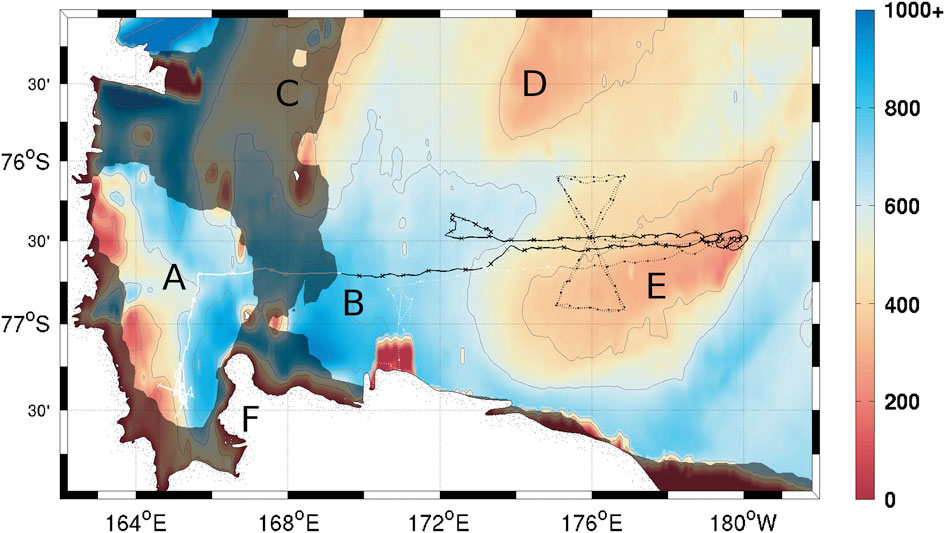
Fig. 1 Seaglider survey locations. Crosses on the solid line show every tenth dive by SG502, circles on the dotted line show every tenth dive by SG503. Dark shading corresponds to the 50% ice cover contour on the day SG502 crossed beneath the ice bridge (14 December 2010) and entered the Ross polynya. Contours correspond to bathymetry in metres (GEBCO 2010). Contours are located at 200 m intervals through 1000 m. a. McMurdo Sound, b. Central Basin, c. Crary Bank, d. Pennell Bank, e. Ross Bank, f. Ross Island.
Both gliders were launched from the ice edge as no other means of launch were available (Asper et al. Reference Asper, Lee, Gobat, Smith, Heywood, Queste and Dinniman2011). Launch conditions did not allow collection of data for calibration and no moorings were available for cross calibration during the survey. This limitation is one that must be accepted to observe the region this early in the season unless small boat capabilities become available from the nearby stations. All glider data were calibrated against a single CTD cast each from the RVIB Nathaniel B. Palmer during recovery on 20 January (SG502) and 30 January (SG503). Salinity and chlorophyll a sensors on the ship’s CTD rosette were calibrated against in situ samples. Shipboard bottle measurements of chlorophyll a were determined via fluorescence on a Turner Designs Model 10 AU fluorometer after filtration and 24 hour extraction in 90% acetone. Fluorescence counts from SG502’s final upcast were regressed with bottle measurements of chlorophyll a during recovery (R2=0.94), and this regression was applied to all glider fluorescence data to determine estimated chlorophyll a concentrations.
Ship DO data were not calibrated using in situ measurements due to high replicate differences in Winkler titrations. The ship’s CTD sensor package was equipped with a Seabird SBE43 sensor that had recently been calibrated; this provided the best calibration data for the Seaglider optodes. For the densest water mass identified for each glider throughout the survey, a linear regression of DO concentrations against time was performed and the resulting slope used as an estimate of sensor drift. This method assumes that the densest water mass identified had constant DO concentrations and was minimally affected by biological production or consumption on the time scales of the study. Figure 2 shows the DO rate of change for waters of different potential temperature and salinity properties after removal of the calculated optode drift. Both SG502 and SG503 show very similar patterns with strong consumption in most water masses, with the exception of the deep stable water mass which was used to estimate and remove sensor drift by shifting all rates to 0 μmol dm-3 day-1.
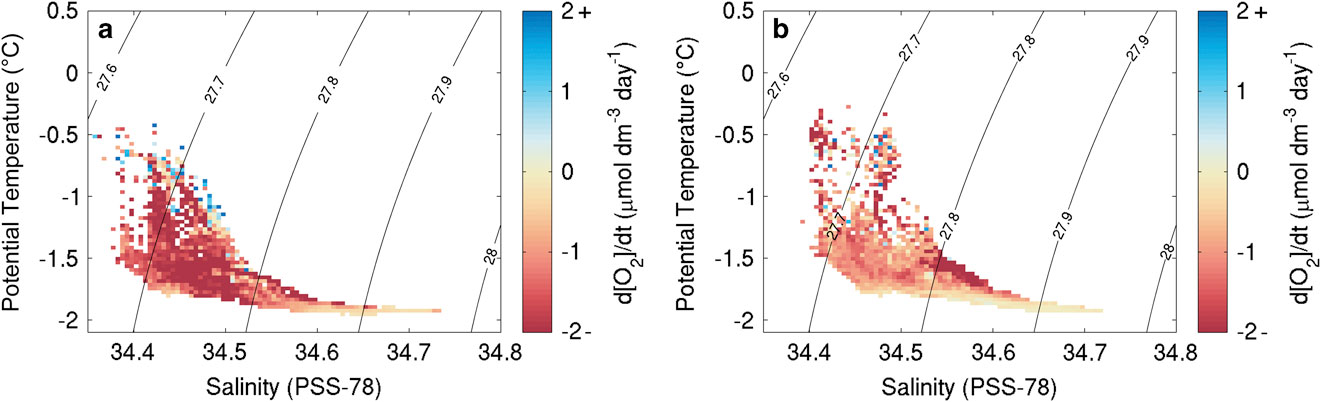
Fig. 2 Dissolved oxygen change for specific temperature and salinity signatures during the bloom from linear regressions of dissolved oxygen concentrations (μmol dm-3 d-1) of data after sensor drift correction (a. SG502, b. SG503).
Erroneous temperature, salinity and DO datapoints due to sensor noise were removed from the analysis using thresholds for reasonable data on the basis of calibrated data and visual inspection. Temperature, salinity, DO and chlorophyll a data were then binned using a regular 3 hr by 3 db grid. Finally, a vertical linear interpolation was used to fill empty bins. All figures use gridded observations rather than individual datapoints. A comparison of raw and gridded data (Fig. 3) showed no discernible differences or aliasing of the raw signal.
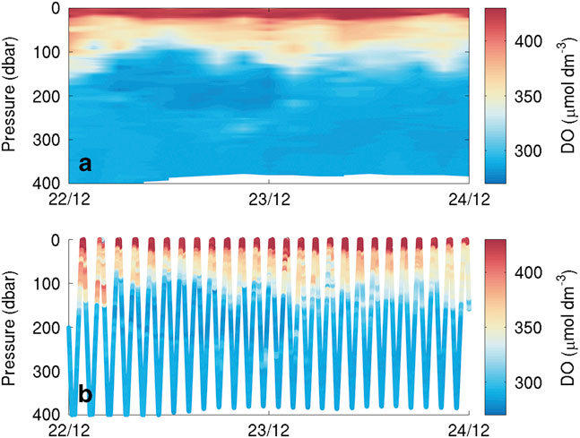
Fig. 3 Short dissolved oxygen (DO) section of the Seaglider transect showing a. data after binning and b. scattered raw data. The binning process maintains all the variability visible in the raw data.
In order to estimate production, the oxygen data within the survey area were analysed as described by Riser & Johnson (Reference Riser and Johnson2008) and Alkire et al. (Reference Alkire, D’Asaro, Lee, Perry, Gray, Cetinić, Briggs, Rehm, Kallin, Kaiser and González-Posada2012). Alkire et al. (Reference Alkire, D’Asaro, Lee, Perry, Gray, Cetinić, Briggs, Rehm, Kallin, Kaiser and González-Posada2012) assessed production during a bloom using floats and gliders. They equated the rate of change of the water column DO inventory to the sum of oxygen fluxes, including biological production and consumption, horizontal and vertical advection, isopycnal and diapycnal mixing and air–sea exchanges:
 $$\eqalignno{{{\Delta [O_{2} ]} \over {\Delta t}}=F_{{biological}} {\plus}F_{{advection}} {\plus}F_{{upwelling}} {\plus}F_{{isopycnal\,mixing}} \cr {\plus}F_{{diapycnal\,mixing}} {\plus}F_{{ASE}} .$$
Alkire et al. (Reference Alkire, D’Asaro, Lee, Perry, Gray, Cetinić, Briggs, Rehm, Kallin, Kaiser and González-Posada2012) used a Lagrangian experimental design and assumed that advection was negligible. Here we assume that temporal changes of DO in the water column during the gliders’ repeated surveys are far greater than any spatial variability that might be aliased into the time series. For the simple calculations presented here, the effects of upwelling and mixing are assumed to be negligible compared with oxygen utilization during the bloom. Therefore, apparent oxygen utilization rates measured below the SML are assumed to be biogenic. Estimation of air–sea exchanges is required for assessing SML rates. A rate of daily DO change was estimated by linearly regressing apparent oxygen utilization (AOU), defined as the difference between the measured DO concentration and saturation concentration against time for each depth bin; within each depth bin the slope of the regression is an estimate of:
 $${{d[O_{2} ]} \over {dt}}.$$
The resulting estimates of production are subject to uncertainty. The largest contributor to uncertainty is in the air–sea exchange calculation where wind speed parameterization and the inclusion of bubble injection can lead to an uncertainty of nearly 40% in air–sea gas transfer estimates (Nightingale et al. Reference Nightingale, Malin, Law, Watson, Liss, Liddicoat, Boutin and Upstill-Goddard2000, Naegler et al. Reference Naegler, Ciais, Rodgers and Levin2006). The other term in the DO budget subject to uncertainty is the observed:
 $${{\Delta [O_{2} ]} \over {\Delta t}},$$
where uncertainty originates from two sources. The first is sensor measurement error and subsequent calculation of DO due to inaccuracies in temperature, salinity, pressure and oxygen optode output (estimated to be 5% by the manufacturer). The second is the linear regression performed for each depth bin. Finally, uncertainty in estimating productivity stems from the estimate of water column depth and the AOU:C ratio, here estimated to be 25%.
Results and discussion
Bloom timing and distribution
SG502 travelled east across Ross Bank before returning to the western Ross Sea (Fig. 1). During the eastward transect, SG502 recorded a deepening of a surface warm layer (25 m; Fig. 4a). Below the surface warm layer and above the 27.8 kg m-3 isopycnal (dashed line in Fig. 4), an intermediate water mass exhibits temperatures warmer than the very cold bottom waters. On the return transect, this same three-layer pattern remained, but with a much thicker surface warm layer extending to 50 m. At the eastern edge of the bank, where depths approach 250 m, the warm surface layer is not present. Salinity does not follow the same vertical distribution as temperature, with a much more gradual decrease from fresher surface waters (34.30 on the PSS-78; 34.47 g kg-1 using TEOS 10) to the saline deep water (34.70 on the PSS-78; 34.87 g kg-1 using TEOS 10) (Fig. 4b). The warm surface layer and fresh surface waters creates a strong pycnocline which deepened from 20 to 50 m over the study period; this pycnocline is not observed at the eastern edge of Ross Bank. Below this SML, isopycnals follow bathymetric contours in regions shallower than 400 m, but shoal away from the bank when depth exceeds 400 m.
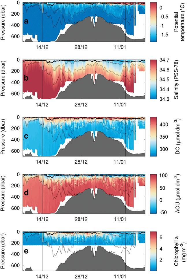
Fig. 4a Temperature (°C), b. salinity, c. dissolved oxygen (DO, μmol dm-3), d. apparent oxygen utilization (AOU, μmol dm-3) and e. chlorophyll a (mg m-3) sections during the bloom observed by SG502 in the Ross Sea polynya. Potential density contours are shown at 0.1 kg m-3 intervals from 27.9 kg m-3 (solid line) to 27.6 kg m-3 (dash-dot line). An estimate of mixed layer depth from Kaufman et al. (Reference Kaufman, Friedrichs, Smith, Queste and Heywood2014) is included as a thick solid line near the surface. The bloom study period is identified by the vertical bars.
SG503 observed a similar temperature and salinity distribution. A thin warm surface layer appears on 21 December and gradually deepens to 60 m. An intermediate water mass is visible down to the 27.8 kg m-3 isopycnal (Fig. 5a). The warm surface layer is observed throughout SG503’s survey, indicating that its absence at the eastern edge of Ross Bank was probably due to increased vertical mixing in the shallow region or strong frontal processes along the eastern edge of the bank. Interestingly, there is little fresh water (< 34.45) visible above the shallower regions of SG503’s transect (Fig. 5b).
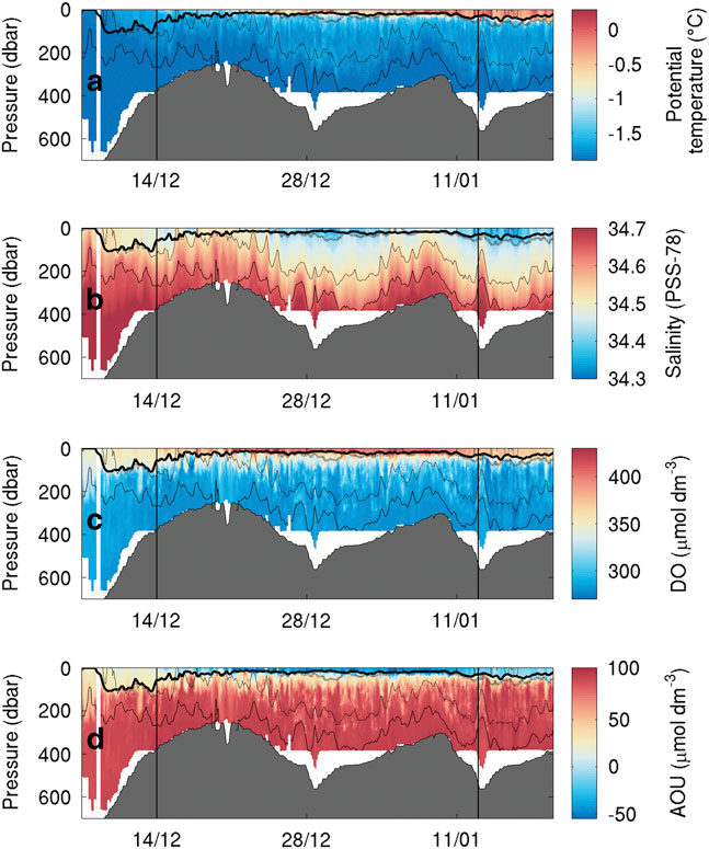
Fig. 5a Temperature (°C), b. salinity, c. dissolved oxygen (μmol dm-3) and d. apparent oxygen utilization (AOU, μmol dm-3) sections during the bloom observed by SG503 in the Ross Sea polynya. Potential density contours are shown at 0.1 kg m-3 intervals from 27.9 kg m-3 (solid line) to 27.6 kg m-3 (dash-dot line). An estimate of mixed layer depth from Kaufman et al. (Reference Kaufman, Friedrichs, Smith, Queste and Heywood2014) is included as a thick solid line near the surface. The bloom study period is identified by the vertical bars.
As the SML thickness was consistent between both SG502 and SG503, it is assumed that this SML was present over a much wider area and its formation governed by large-scale processes, such as increasing solar radiation and changing wind speeds. Wind speeds above the location of each glider (Fig. 6a) suggest that the greater winds at the start of the mission prevented the formation of a stable SML. Subsequently, lower wind speeds appear to have remained spatially consistent over both gliders. Another strong wind speed event (>10 m s-1) began on 8 January but had little visible impact on water column density structure (Figs 4 & 5). At the same time, SG502 and SG503 observed different isopycnal depths, implying a strong spatial dependence. This is interpreted as geostrophic currents following bathymetric contours causing spatial variability in isopycnal depth. These geostrophic flows advect biogeochemical properties and are associated with fronts contributing to a strong physical and chemical heterogeneity in the western Ross Sea polynya.
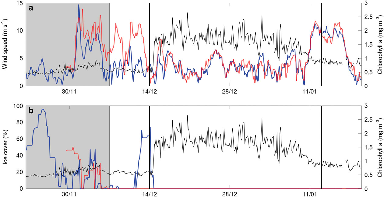
Fig. 6a Mean chlorophyll a concentration (mg m-3) through the top 250 m of SG502’s observations (black line) and wind speed (ECMWF ERA interim at 10 m, m s-1) over the location of SG502 (solid blue line) and SG503 (red dashed line). b. Mean chlorophyll a concentration and percentage ice cover from SSMIS imagery with the colours as in panel a. Vertical black lines indicate bloom initiation and end of the analysis period. The shaded portion of the figure shows conditions of wind and ice cover before the analysis period and is included for context to indicate the timing of the polynya opening.
Chlorophyll a fluorescence data were only recorded in the top 250 m for SG502 (Fig. 4d). A large bloom is observed within the Ross polynya while SG502 surveyed the Ross Bank. Chlorophyll a concentrations peaked at 7 mg m-3, with the majority of the bloom showing subsurface maxima of 4 mg m-3 at approximately 40 m depth and elevated chlorophyll concentrations between 10 and 65 m. Observed chlorophyll a concentrations decreased rapidly after 5 January when SG502 began the westward transect. Fig. 7 shows a 30-day composite of satellite ocean colour derived chlorophyll a concentration when SG502 observed the bloom over Ross Bank (14 December to 13 January). Despite averaging satellite data over a month, a large area is devoid of data due to extensive cloud and ice cover. Nonetheless, an extensive bloom similar to that observed by the Seaglider is revealed (4–7 mg m-3) extending into the Central Basin. The satellite data indicate that the bloom was not spatially constrained, at least at the surface, to only the Ross Bank, but was also present in the Central Basin region.
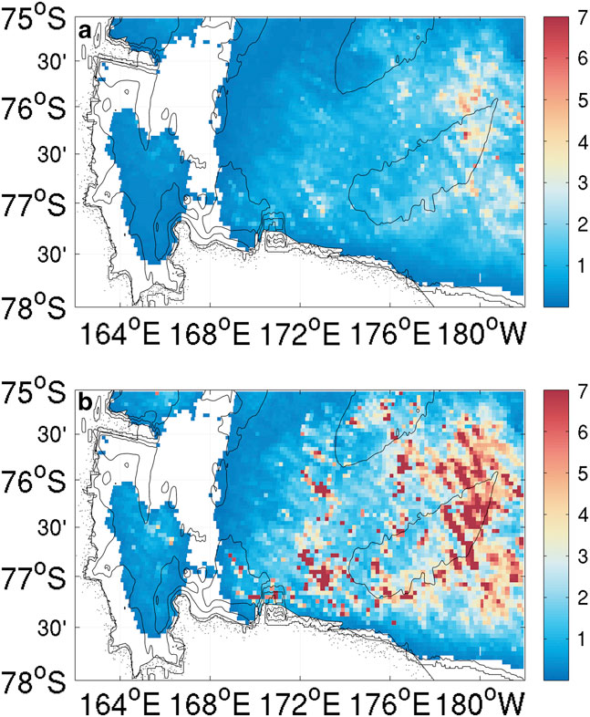
Fig. 7a Mean and b. maximum values of a 30-day composite of MODIS ocean colour surface chlorophyll a concentrations (mg m-3) from the 14 December 2010 to 13 January 2011. White areas are devoid of data due to the continuous cloud and ice cover during this period.
As this bloom included both the banks and basin (Fig. 7), it is not likely that its onset is regulated by advective processes, such as mesoscale intrusions of MCDW, as this would cause enhanced localized chlorophyll maxima along the edges of the bank (Kohut et al. Reference Kohut, Hunter and Huber2013). The onset of the bloom in the Ross Sea polynya is traditionally considered to be initiated by increased irradiance, vertical stability and iron release in the water column due to ice melt (Sedwick & DiTullio Reference Sedwick and DiTullio1997, Smith & Gordon Reference Smith and Gordon1997, Smith & Comiso Reference Smith and Comiso2008). Figure 6a compares wind velocity above SG502 and chlorophyll a concentrations in the top 50 m. A week after wind speeds decrease below 5 m s-1, an increase in chlorophyll a was observed. There was a two week period between the first period of surface ice melt (1 December) and the onset of the bloom (Fig. 6b). The onset of the bloom cannot be directly attributed to either a decrease in winds or ice melt as ice was present immediately after wind speeds decreased and no increase of biomass was visible immediately after the first period of ice melt.
Overall, these results indicate that the factor delaying the onset of the bloom was a lack of vertical stability in the water column. Once the ice receded, sufficient nutrients and light were available for phytoplankton growth, but strong wind speeds prevented the phytoplankton from growing in a stratified water column and optimal light regime. Once wind speeds decreased, surface warming accelerated stratification of the surface layer, allowing the phytoplankton to grow and accumulate (Fig. 4). Such rates of increase are consistent with known growth rates in the Ross Sea (e.g. Smith et al. Reference Smith, Shields, Peloquin, Catalano, Tozzi, Dinniman and Asper2006). Hence, ice melt is not the sole control of stratification in the region; strong winds also play a role in controlling the onset of the stratification of the water column. Both conditions need to be met to trigger the onset of the bloom.
The bloom ended during the first week of January with strong mixing of the water column and a redistribution of chlorophyll a (Fig. 4d), as shown by the reduction in chlorophyll a concentrations and the appearance of the chlorophyll maximum at depth (150 m). These occurrences coincide with the second greater wind speed event (>10 m s-1; Fig. 6a) and a deepening of the mixed layer depth from c. 15 to 35 m. This agrees with observations by Smith et al. (Reference Smith, Shields, Dreyer, Peloquin and Asper2011b) that mixing events may cause bloom termination in the Ross Sea polynya. More detailed observations of the mechanisms regulating variability during the demise of this bloom are described by Kaufman et al. (Reference Kaufman, Friedrichs, Smith, Queste and Heywood2014).
Dissolved oxygen distribution
There is net consumption of DO during the survey within most water masses present (Fig. 2). Peak DO consumption occurs both in surface waters and in intermediate waters along the 27.8 kg m-3 isopycnal. Despite overall consumption, there is a net increase in surface DO during the first half of the survey (Figs 4c, 5c & 8). The DO consumption was consistent with a surface layer of oxygen supersaturation (negative AOU) down to 50 m for both gliders. As the warm SML appeared, it exhibited supersaturation of DO (Fig. 8). Peak DO concentrations were observed by both gliders between 21 December and 1 January (Figs 4c, 5c & 8). Fluctuations in surface saturation were synchronous between the gliders (Fig. 8). Finally, surface saturations decreased during the final two weeks of the mission as the gliders surveyed the region west of the Ross Bank (west of 175°E). This period reflected a substantial increase in particulate organic carbon that was attributed to a secondary diatom bloom in the same location as the oxygen increase (Kaufman et al. Reference Kaufman, Friedrichs, Smith, Queste and Heywood2014).
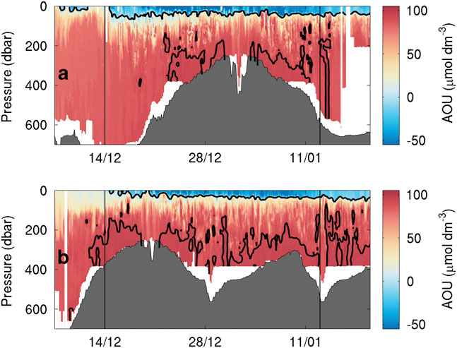
Fig. 8 Apparent oxygen utilization (μmol dm-3) as observed by a. SG502 and b. SG503. To highlight supersaturation threshold and peak consumption regions, 0 and 92 μmol dm-3 contours have been added.
The AOU varies in both time and space (Fig. 8). It is used here instead of DO concentration to allow for the effects of physical changes, particularly temperature on oxygen saturation. It illustrates both supersaturation (negative AOU) and undersaturation (positive AOU). Observations from both SG502 and SG503 show increasing AOU towards the bottom of the water column (Fig. 8). Consumption (i.e. positive AOU) above 90 μmol dm-3 is constrained to regions deeper than 400 m according to SG502 (Fig. 8a). It is probable that sinking organic matter from the phytoplankton bloom is remineralized gradually and is deposited on the seabed; this remineralization requires the consumption of DO and often leads to reduction of bottom mixed layer DO (Queste et al. Reference Queste, Fernand, Jickells and Heywood2013). Further consumption, within the nepheloid layer and during resuspension of settled organic matter, increases AOU near the seabed. In regions deeper than 400 m, the impact of remineralization of organic matter on the oxygen inventory is reduced as there is a larger reservoir of DO. Additionally, the greater depth means more organic matter is remineralized as it sinks rather than once it has settled on the seabed. This consumes oxygen throughout the water column rather than concentrating the oxidation near the seabed.
Following these observations of biogenic DO variability, a depth integrated budget of DO production over time was derived (Fig. 9). Production is maintained within the top 50–70 m of the water column within an SML of gradually changing density. A peak in oxygen production was observed at 30 m, decreasing near the surface and switching to a net consumption regime below 50 m. The surface decrease is probably due to degassing of DO when the SML is supersaturated. Maximum oxygen production correlates with maximum observed chlorophyll a concentrations (Fig. 9b), suggesting primary production within the deep chlorophyll maximum (DCM) as the cause. Below the DCM, chlorophyll a concentrations decreased gradually and remained relatively high (>1.5 mg m-3) throughout the upper 100 m. This suggests that phytoplankton sank from the euphotic zone and served as a significant source of organic matter to depth. Simultaneously, a sharp decrease in DO below the DCM was observed. Peak apparent consumption occurs at 70 m in both regions. The consumption of DO is strongest just below the DCM and gradually decreases to modest DO consumption rates. This indicates that the majority of organic matter produced within the euphotic zone is rapidly remineralized before it reaches 200 m, consistent with particulate organic carbon distributions (Kaufman et al. Reference Kaufman, Friedrichs, Smith, Queste and Heywood2014) and with studies performed in other regions around Antarctica (Weston et al. Reference Weston, Jickells, Carson, Clarke, Meredith, Brandon, Wallace, Ussher and Hendry2013). However, this contrasts with the substantial oxygen removal near the seabed (Fig. 8). It is possible that an older water mass moving along the bank could contribute to the high AOU observed near the seabed. Kohut et al. (Reference Kohut, Hunter and Huber2013) and Kaufman et al. (Reference Kaufman, Friedrichs, Smith, Queste and Heywood2014) both report the presence of MCDW along Ross Bank during the 2010–11 summer; this water mass can be identified by its lower oxygen concentration and its unique temperature/salinity features (Orsi & Wiederwohl Reference Orsi and Wiederwohl2009). However, the elevated AOU was probably caused by consumption earlier in the season through resuspension of organic matter deposited on the seabed, allowing for slow but continuous consumption (Nelson et al. Reference Nelson, DeMaster, Dunbar and Smith1996). Further study of the cause of near-bed oxygen depletion on Ross Bank would be useful.
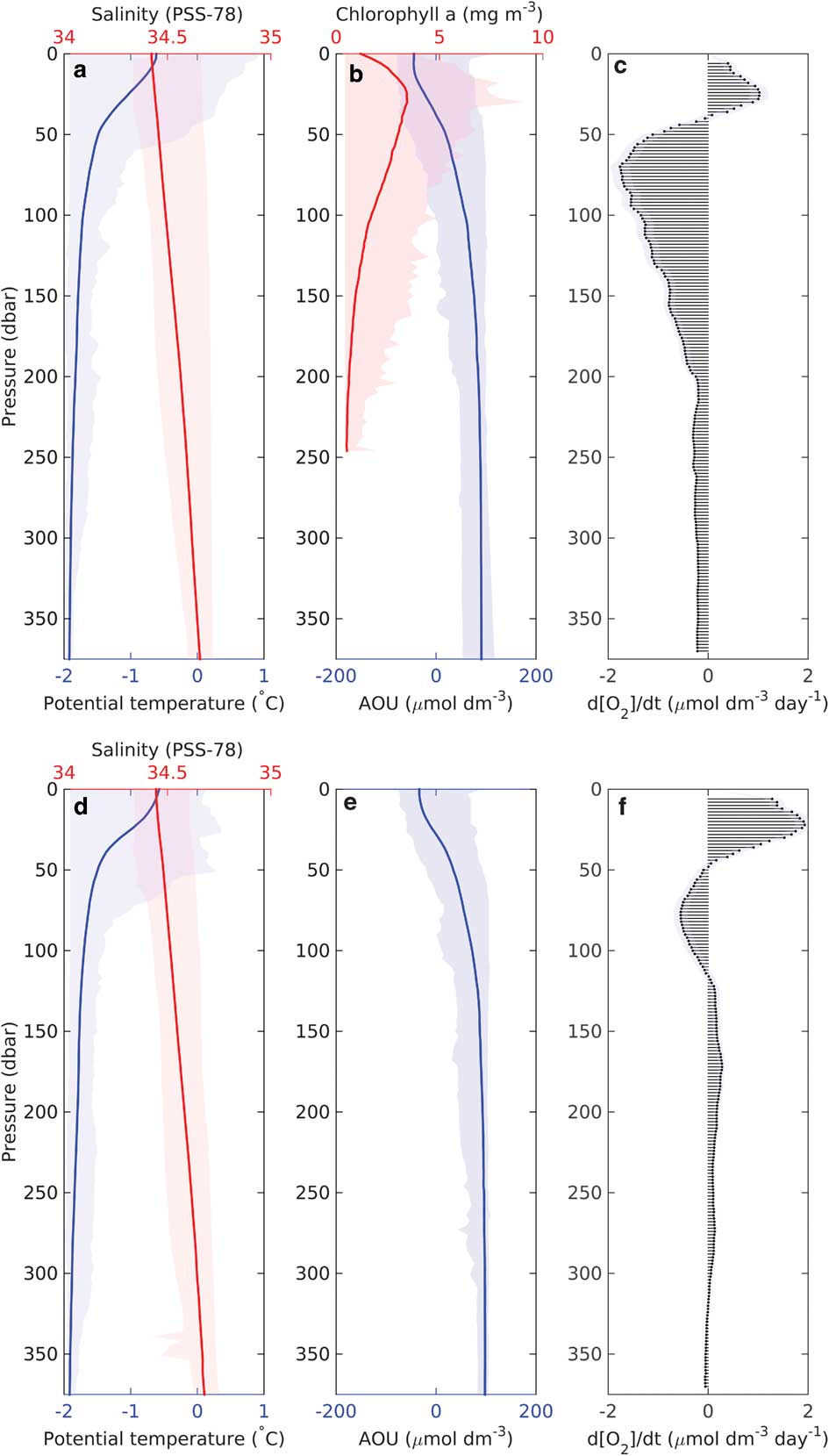
Fig. 9a & d. Mean vertical profiles of potential temperature (°C, blue) and salinity (red), b. & e. apparent oxygen utilization (AOU, μmol dm-3, blue) and chlorophyll a (mg m-3, red) during the bloom identified by SG502 (top) and SG503 (bottom). Total variability of the profiles (minimum to maximum extent) is displayed as a lighter shade for each variable. c. & f. Vertical distribution of dissolved oxygen change over time (μmol dm-3 d-1), as estimated by linear regressions for each depth bin for SG502 (top) and SG503 (bottom). Shading indicates one standard deviation for the regression of the rate.
In the calculation of biogenic rates of oxygen change, both the effects of upwelling and horizontal advection are neglected. Upwelling can be neglected as the entire water column is resolved in glider observations, although it may have a small impact on the vertical distribution of rates in Fig. 9. Including the effects of upwelling into the calculations would not affect depth integrated estimates of productivity. Entrainment of water with different DO could contribute to the overall DO change over time observed. However, it is not possible to estimate the horizontal gradient in DO. While it is possible to resolve mean water column current direction from the glider data, true entrainment cannot be resolved due to the confounding impacts of tides and transient flows. Entrainment of water with different DO would probably also vary vertically, and resolving this vertical variability of horizontal advection is not possible with the glider data. However, any potential effect of entrainment is probably small and non-systematic. While the glider’s travel relative to water can increase uncertainty in measurements of in situ oxygen consumption by not behaving as a Lagrangian platform, the large distances travelled and the repeated transects negate the bias caused by spatially dependent factors.
The standard deviation for the regression of the slope was 0.10 for SG502 and 0.07 for SG503 (shading on Fig. 9a & b). Mean dissolved oxygen change over time in the water column was -0.50±0.1 μmol dm-3 d-1 for SG502 and 0.15±0.07 μmol dm-3 d-1 for SG503. Assuming a water column depth of 400 m, this amounts to -0.20±0.04 and 0.060±0.03 mol m-2 d-1 over the whole water column. Generally, AOU:C ratios are between 0.5 and 2.0, with productive shelf seas closer to the latter value (Thomas Reference Thomas2002). Using an AOU:C ratio of 2:1, this would suggest production rates of -0.10±0.04 mol C m-2 d-1 and 0.030±0.02 mol C m-2 d-1. In the absence of air–sea exchange, the observed DO change over time would indicate net community production of -1.2±0.5 g C m-2 d-1 for SG502 and 0.36±0.2 g C m-2 d-1 for SG503. As the surface layer is supersaturated (Fig. 8), air–sea gas exchange will lead to the rapid loss of excess DO from the SML. Air–sea gas exchange depends on the concentration gradient in surface waters and a gas exchange rate, which is wind speed and temperature dependent. Estimates of sea to air oxygen flux based on wind speeds from the European Centre for Medium-Range Weather Forecast ERA-interim (ECMWF ERA), Seaglider measurements of surface temperature, salinity and DO and using an empirical fit to dual tracer data by Johnson (Reference Johnson2010) and Nightingale et al. (Reference Nightingale, Malin, Law, Watson, Liss, Liddicoat, Boutin and Upstill-Goddard2000) are c. 0.025 mol m-2 d-1 (Fig. 10; $\bar{x}$
=0.0239 mol m-2 d-1). By including an air–sea flux of 0.025±0.01 mol m-2 d-1 (an additional 0.3±0.2 g C m-2 d-1), net community production rates estimated from the observations of SG502 and SG503 are -0.9±0.7 and 0.7±0.4 g C m-2 d-1, respectively.
$\bar{x}$
=0.0239 mol m-2 d-1). By including an air–sea flux of 0.025±0.01 mol m-2 d-1 (an additional 0.3±0.2 g C m-2 d-1), net community production rates estimated from the observations of SG502 and SG503 are -0.9±0.7 and 0.7±0.4 g C m-2 d-1, respectively.
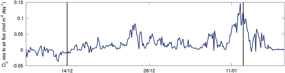
Fig. 10 Sea to air flux of dissolved oxygen (DO, μmol dm-2 d-1) based on ECMWF ERA interim wind speeds, Seaglider measurements of surface temperature, salinity and DO and using an empirical fit to dual tracer data by Nightingale et al. (Reference Nightingale, Malin, Law, Watson, Liss, Liddicoat, Boutin and Upstill-Goddard2000) and Johnson (Reference Johnson2010).
Conclusions
It is difficult to reconcile the two different glider estimates of production, as both gliders were observing the western Ross Sea polynya during the same time period. The main sources of uncertainty in the estimates are the assumption of horizontal homogeneity and the estimation of air–sea exchanges. Furthermore, a value of two for the AOU:C ratio is an upper boundary; this implies that absolute values of carbon production and consumption are probably greater than derived here. However, despite having to make these assumptions, we still gain greater insight into the DO dynamics, and particularly the high variability of DO dynamics, in this region. The contrasting results of SG502 and SG503, the former showing net consumption and the latter net production, highlight that this is a highly variable region, exhibiting both net production and net consumption depending on the time and region. The sinking event observed by SG502 at the end of the bloom probably had a disproportionate effect on the calculation of rates. If this sinking event was related to topographically induced flows along the bank, it is possible that the oxygen depletion signature caused by rapid remineralization of the sinking organic matter affected the calculation of rates from SG502 data differently to the data from SG503. Alternatively, the bloom’s demise may occur at different times across the survey region. The satellite imagery showed significant differences in bloom intensity either side of the bank.
It is probable that data from SG502 illustrate a more advanced stage of the bloom’s demise when production has greatly decreased in the SML and respiration has greatly increased as the biomass sinks to depth. Data from SG503 represent an earlier stage of the bloom, when production was occurring at a much greater rate within the SML and the phytoplankton assemblage was maintained within the SML, leading to only limited remineralization in the sub-euphotic depths of the water column.
This mission served to demonstrate the substantial value of autonomous underwater gliders in remote regions such as the Ross Sea. These instruments provided a wealth of observations, with greater spatial and temporal resolution than any shipboard survey. Autonomous underwater gliders could greatly increase our understanding of the region’s biogeochemical cycles and the influence of small and mesoscale processes on these cycles, and further oceanographic programmes would benefit from the merger of a variety of sampling platforms to resolve the temporal and spatial variability observed.
Acknowledgements
Bastien Queste was funded by a NERC CASE PhD studentship and an Antarctic Science International Bursary (http://www.antarcticsciencebursary.org.uk). This work was funded by the National Science Foundation’s Office of Polar Programs (NSF-ANT-0838980). Michael Dinniman was funded by US National Science Foundation grant NSF-ANT-0838948. We acknowledge funding support from NERC grant GENTOO (Gliders: Excellent New Tools for Observing the Ocean, NE/H01439X/1). We thank Craig Lee, Jason Gobat and Vernon Asper for technical assistance and help with the Seagliders. This paper is Contribution No. 3418 of the Virginia Institute of Marine Science, College of William & Mary. Bathymetric data were obtained from the GEBCO_08 Grid, version 20100927. Wind and atmospheric data were obtained from the European Centre for Medium-Range Weather Forecasts (ECMWF). Satellite chlorophyll data were obtained from the Ocean Biology Processing Group (OBPG) at the Goddard Space Flight and sea ice data from the Special Sensor Microwave Imager/Sounder of the US National Snow and Ice Data Center. We would like to thank our reviewers, Dr Elizabeth Shadwick and the Antarctic Science editorial team for their hard work and helpful comments.
Author contribution
W.O.S. and K.J.H. designed the study and provided the Seagliders. B.Y.Q. corrected and interpreted the data and wrote the paper. All authors contributed significantly to the interpretation of the data and revisions of the manuscript.


 Open access