


Introduction
Global mean surface air temperature has increased by ~0.74°C over the past 100 years, and is predicted to rise an additional 1.1-6.4°C by the end of the present century (Reference SolomonSolomon and others, 2007). This warming has influenced alpine glacier fluctuation and runoff, resulting in annual mass losses of up to 3 ma–1 (e.g. the European Alps; Reference Zemp, Frauenfelder, Haeberli and HoelzleZemp and others, 2005). Glacier mass loss is expected to continue, and simulations based on climate warming from greenhouse gases predict a 20% increase in mean annual discharge of the great Arctic rivers (Reference Macdonald, Harner and FyfeMacdonald and others, 2005). In China, 82.2% of all monitored glaciers have retreated, with a total area loss of 4.5% from the 1950s to the late 1990s (Reference Liu, Ding, Li, Shangguan and ZhangLiu and others, 2006).
Because warming-induced alpine glacier melting is likely to intensify, water-rock interactions such as sulfide oxidation and carbonate dissolution are also expected to increase. Glaciation is responsible for a significant drawdown of atmospheric CO2, generating a negative feedback on climate (Reference Sharp, Tranter, Brown and SkidmoreSharp and others, 1995; Reference Tranter and BottrellTranter, 1996; Reference Hodson, Porter, Lowe and MumfordHodson and others, 2002; Reference Yde, Knudsen and NielsenYde and others, 2005; Bartoszewski, 2008). It has long been recognized that rates of terrestrial chemical erosion may influence the atmospheric concentration of CO2, a radiatively important gas contributing to mean global temperature regulation (Reference Raymo and RuddimanRaymo and Ruddiman, 1992). Because of its potential impact on climate at glacial-interglacial timescales, CO2 sequestration during episodes of deglaciation has attracted considerable attention (Reference BrownBrown, 2002).
Research on carbon dioxide drawdown in glaciated catchments has been launched in recent years (Reference Hodson, Porter, Lowe and MumfordHodson and others, 2002; Reference Yde, Knudsen and NielsenYde and others, 2005; Reference Krawczyk and BartoszewskiKrawczyk and others, 2008; Reference Roberts, Yde, Knudsen, Long and LloydRoberts and others, 2008). However, these studies have been almost entirely reliant on the ionic mass-balance method of carbon dioxide flux calculations, without direct CO2 concentration and flux monitoring systems. Moreover, eddy covariance data of CO2 flux have been collected over the horizontal surfaces of large ice bodies (Reference Mölg, Hardy and KaserMölg and others, 2003; Reference Cullen, Mölg, Kaser, Steffen and HardyCullen and others, 2007; Mac-Donell and others, 2010; Reference Jarosch, Anslow and SheaJarosch and others, 2011) and in complex terrain (Reference Rotach, Calanca, Weigel and AndrettaRotach and others, 2003; Reference Hiller, Zeeman and EugsterHiller and others, 2008; Reference GuoGuo and others, 2011; Reference JocherJocher and others, 2012). Such an approach may be unsuitable for the study of alpine glaciers, given complex terrain, frequent precipitation and fog, and other factors. The gradient method for collecting and calculating CO2 flux has been used to study net CO2 exchange with the atmosphere in a wide variety of terrains (snow, grassland, forest, bare land, and alpine) (Reference SteffenSteffen and others, 2008; Reference Bowling and MassmanBowling and Massman, 2011; Reference Pumpanen, Kulmala, Bäck, Lappalainen and NieminenPumpanen and others, 2011), including complex terrains. Thus, the gradient method may be useful for the study of processes underlying CO2 exchange between the atmosphere and a glacial surface, providing continuous data without interference from precipitation, fog and refrozen condensed water (Reference Bowling and MassmanBowling and Massman, 2011; Reference Pumpanen, Kulmala, Bäck, Lappalainen and NieminenPumpanen and others, 2011).
Using the mass-balance method, total solute fluxes and transient carbon dioxide sinks (which accounted for 14.2% of total solutes in bulk river water) were estimated at 791.2 kg (km 2 d)–1 and 81.0 kg (km2 d)–1 in the Koxkar glaciated basin (summer 2004), respectively (Reference Wang, Xu, Zhang, Liu and HanWang and others, 2010). Using the flux gradient method, this paper aims to estimate CO2 fluxes over bare ice and supraglacial moraine at Koxkar glacier during the 2012 melt season. These results, together with other data, may shed light on the influence of atmospheric factors on CO2 fluxes. Specifically, these data provide new insight into CO2 concentrations and fluxes in glaciated basins, which may be used for modeling CO2 change on glacial–interglacial timescales (e.g. Reference TranterTranter and others, 2002). A further aim is to seek correlations between CO2 flux and other factors across different underlying surfaces on Koxkar glacier, which may facilitate conclusions regarding the feedback relationship of glacial change to regional atmospheric CO2 circulation.
Site Description
The glaciated Koxkar basin (41842’–41853’ N, 79859’– 80810’E; Fig. 1) is on the southwest side of Toumuer mountain, northwest China. The glacier is 25.1 km long and has an area of 83.56km2. Supraglacial debris covers -15.6 km2, representing 83% of the total ablation area (Reference Han, Wang, Wei and LiuHan and others, 2010). Mean annual air temperature observed near the glacier terminus is 0.77°C, and mean summer temperature is 7.74°C (Reference HanHan and others, 2008). The main source of precipitation is water vapor from the Atlantic and Arctic Oceans (Reference Kang, Zhu and HuangKang and others, 1985). Annual precipitation, 81% of which occurs from May through September, is ~630 mm at the end of the glacier. Precipitation in the study area is in a solid state (snow and hail). A field investigation from 2003 to 2012 indicated annual discharge at the glacial terminus of >1.0 x 10⁸m3, mainly during the warmer half of the year (94.5% of total runoff flux was from May through October).
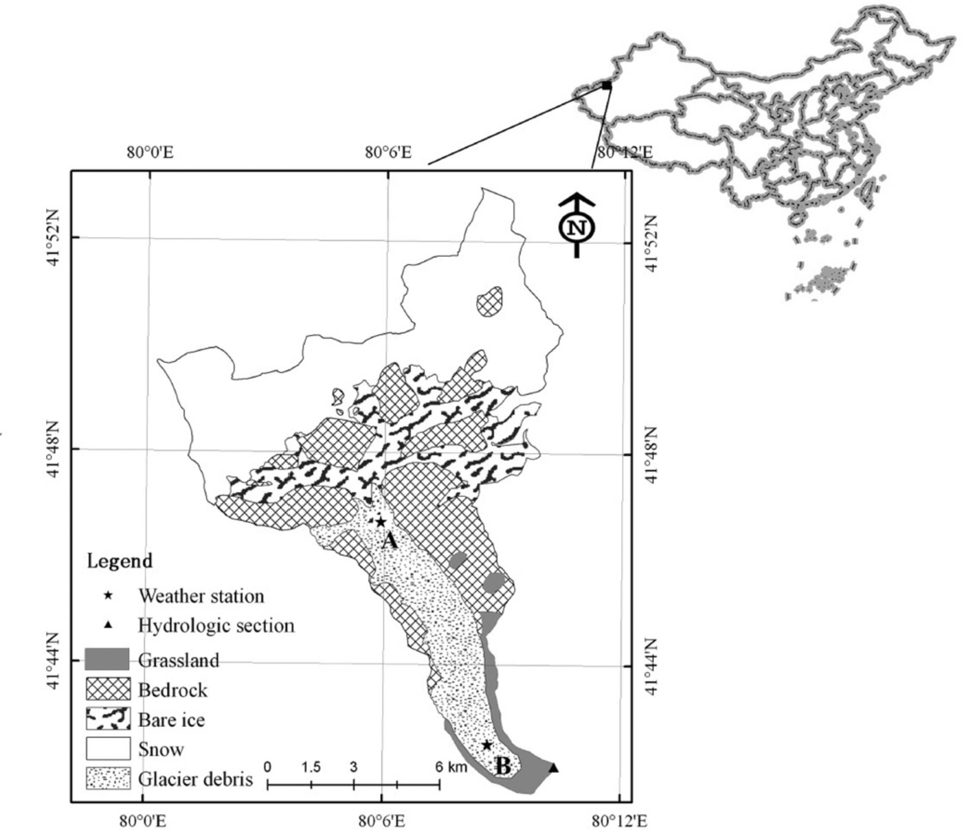
Fig. 1. Map of the Koxkar glacier region (northwest China) sampling sites.
Two CO2 flux gradient observation stations (Fig. 1) sit atop bare ice (site A: 41°47ʹN, 808060E; 3730ma.s.l.) and supraglacial moraine (site B: 418430N, 80°09ʹE; 3212ma.s.l.). Debris thickness at site A is <0.01 m and discontinuous, while the thickness at site B is ~0.70 m. The debris is mainly gray or dark-gray granite stone powder, broken stone particles, and rock mass, which covers 83% of the total melt area. Therefore, moraine is the principal physical source of crustal dissoluble ions. The nearly horizontal surfaces at sites A and B have an average surface slope less than 28, and a fetch of several hundred meters in the direction of the prevailing wind, which most often should be a valley-mountain breeze.
Methods
During the observation period, we established two synchronous gradient observational systems to measure two-tiered CO2 concentrations, wind speed, wind direction, temperature and humidity (2.0 and 1.0 m above the surface), and a series of radiation sensors that included total solar radiation, net radiation and reflection radiation in bare-ice and supraglacial moraine regions. Supraglacial two-tiered CO2 concentrations (2.0 and 1.0 m above the surface) were determined using infrared CO2 sensors (ES-D type, Sense Air, Sweden), with a variance of ±5.4% for CO2 (Reference Rinne, Tuovinen, Laurila, Hakola, Aurela and HypénRinne and others, 2000; Lu and others, 2010; Reference Fang, Shi, Lu and ChenFang and others, 2011). Data (e.g. CO2 concentration, wind speed, wind direction, temperature, humidity, total solar radiation, net radiation, reflection radiation, and precipitation) were obtained using a PC-3 data acquisition system, and were automatically updated hourly throughout the observation period. Generally, the effective distance was less than ten times the height of the equipment probes. Our gradient observational stations were located in the central part of the glacier, away from nearby grasslands (-1.43 km away), to reduce the possibility of the grassland affecting the CO2 measurement. Unfortunately, we could not obtain synchronous data because of complications with the solar power supply.
The net glacier-system CO2 exchange (NGE) rate between the glacier surface and atmosphere for the temporally and spatially integrated net glacier system is defined as
where Fc is its vertical flux (upward flux being positive) and S is the change of CO2 storage below the CO2 infrared sensors.
We applied the gradient method, in which vertical CO2 fluxes at the glacier surface are estimated by the aerodynamic gradient method (e.g. Reference Sutton, Pitcairn and FowlerSutton and others, 1993). The flux Fc of a component with concentration c is calculated from the product of friction velocity u* , and a concentration scaling parameter c * as (Reference Rinne, Tuovinen, Laurila, Hakola, Aurela and HypénRinne and others, 2000; Reference LoubetLoubet and others, 2013)
where u, and c. are derived from the stability-corrected gradients of wind speed (u) and CO2 concentration (c) vs height (z):
where d is the zero plane displacement height, which represents the shift in aerodynamic ‘ground’ because of the presence of the glacier surface, z is the mounting height of the sensors (2 m), k is the von Kármán constant with values between 0.35 and 0.43 (usually 0.4), and m is the integrated stability correction function for momentum.
Reference Harman and FinniganHarman and others (2008) developed an analytical transfer model for the roughness layer that includes two displacement heights; the model was extended by Reference Siqueira and KatulSiqueira and Katul (2010) to account for stomatal regulation and soil respiration. Reference Harman and FinniganHarman and others (2008) showed that these additional functions would lead to an additional integral term H in the concentration profile, which in turn would lead to a new approximation of the concentration scaling parameter c* :
Reference Siqueira and KatulSiqueira and Katul (2010) give the following expression for 𝜓H:

where Sn is the Schmidt number, (β = c*/uh, dc and dm are the scalar and momentum displacement heights, and c 2c is a constant that can be taken as 1 in the first approximation. More details of 𝜓 m, dc and dm are provided by Benjamin and others (2013).
The value for S was calculated from vertical CO2 concentration profiles (Reference Aubinet, Chermanne, Vandenhaute, Longdoz, Yernaux and LaitatAubinet and others, 2001; Reference AraújoAraújo and others, 2010
where P a is atmospheric pressure, R is the molar gas constant, T a is the air temperature (K), h m is the maximum measurement height above ground level (m), c is the CO2 concentration, t is time (s), and z is the height about ground level (m). Details of the S calculation are provided by Reference ValentiniValentini and others (2000) and Reference KowalskiKowalski (2008).
Results
CO2 fluctuations
Typical fluctuations in hourly CO2 concentration, atmospheric temperature and wind speed measured 2m above bare ice and supraglacial moraine are shown in Figure 2. Mean wind velocity during the observation periods was 2.3 ms–1 at both stations. Mean temperatures were 3.4°C and 7.6°C, and the amplitudes of dominant fluctuation in CO2 concentration were ~439.3 and 472.1 mgm–3 for sites A and B, respectively. Variations in CO2 concentration gradually decreased, followed by increasing atmospheric temperature, which otherwise only gradually increased. For example, there is strong negative correlation between CO2 concentration and atmospheric temperature at site A. The associated equation is
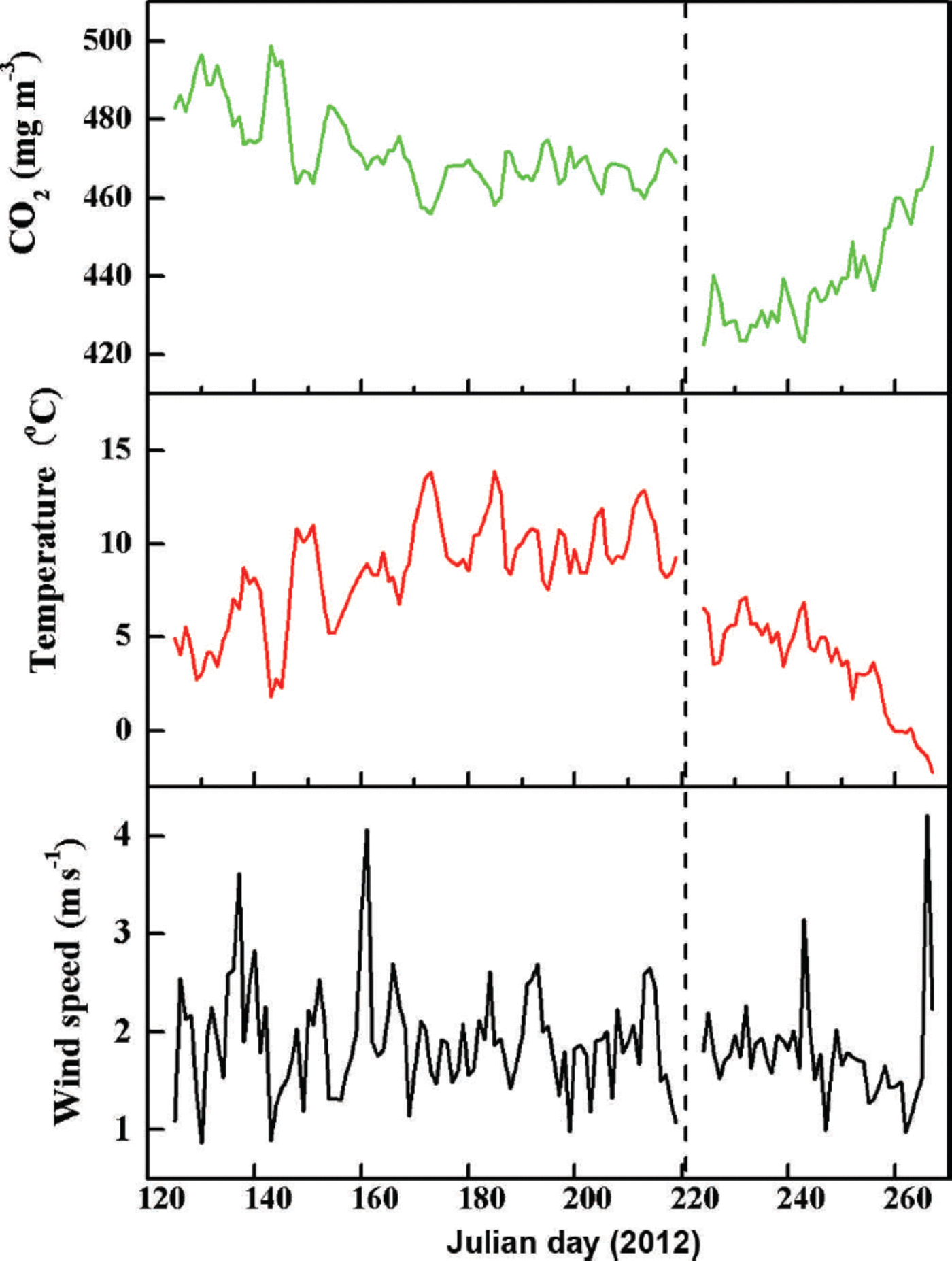
Fig. 2. Fluctuations of hourly CO2 concentration, atmospheric temperature and wind speed above the surface of Koxkar glacier. Data are from bare ice (site A, right of the vertical dotted line) and above supraglacial moraine (site B, left of the vertical dotted line).
where C CO2 is the CO2 concentration (mgm–3), and Tatm is atmospheric temperature (°C) measured 2 m above the ice surface.
Based on Eqns (7) and (8) for site B, the CO2 concentration was less influenced by atmospheric temperature. Equation (8) shows the relationship between CO2 concentration and atmospheric temperature at site B:
Unfortunately, data from sites A and B were not collected simultaneously during the observation period. However, we conclude that the CO2 concentration at site A was dramatically lower than at site B (Fig. 2). This can be explained by the different altitudes and underlying surface conditions at the two sites.
Net glacier-system CO2 exchange (NGE) rate
During the observation period, hourly NGE ranged from –0.74 to +0.48 mmol m–2 s–1 at site A and from –1.81 to +0.66 mmol m–2 s–1 at site B (Table 1). Amplitudes of dominant hourly NGE fluctuation were approximately –0.05 and –0.07 mmol m–2 s–1 for the bare-ice and supraglacial moraine observation points, respectively. These variance results suggest that the fluctuation range of NGE at the supraglacial moraine (site A variance = 60.70) was greater than at bare ice (site B variance = 33.07). Moreover, the maximum and minimum values of hourly NGE were both recorded at site B. Under normal conditions, upward flux (i.e. CO2 release) occurs with precipitation or at night, when ice melt decreases because of reduced air temperature.
Table 1. Hourly NGE (mmol m–2 s–1) at sites A and B on the surface of Koxkar glacier in 2012
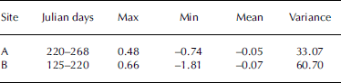
The negative mean values of hourly NGE at the two sites imply that the glacial surface was a sink for atmospheric CO2 during the melt season because of the hydrochemical conditions and mineralogical reactions existing under the ice-melt water (Reference Hodson, Porter, Lowe and MumfordHodson and others, 2002 ; Reference TranterTranter and others, 2002; Reference Yde, Knudsen and NielsenYde and others, 2005; Reference Krawczyk and PetterssonKrawczyk and others, 2007, 2008; Reference Lerman, Wu and MackenzieLerman and others, 2007). In glaciated regions, these chemical reactions are primarily carbonate and silicate dissolution, for example:
Although there was a little cryoconite at the bare-ice site, there were limited amounts of carbonate, silicate and other soluble materials, which could inhibit chemical reactions such as those described by Eqns (9) and (10). Substantial glacial debris at the supraglacial moraine site, including abundant carbonate, silicate and potash/soda feldspar, generated ample chemical hydrolysis under precipitation or ice/snow meltwater conditions. Such mineral differences between sites can account for the differences in hourly NGE rates.
Discussion
Errors in the NGE calculation
In the past, errors in the aerodynamic gradient method used to calculate the atmospheric H2O/CO2 flux have been extensively studied for sites in such locations as grassland, forest, tundra and farmland (Reference Wenzel, Kalthoff and HorlacherWenzel and others, 1997; Reference De RidderDe Ridder, 2010). In the Koxkar glaciated area, the main factors that influenced NGE accuracy were as follows:
-
1. The variance, ±5.4%, of CO2 measured by infrared sensors was an objective value, which might cause 4.8-7.2% error in the NGE result, with a mean value of 5.3%. The sequential sampling of gas concentrations, sourced from ice melting, at various heights above the ice showed a variability in the gradients due to the non-stationarity of the concentrations. These were obviously not an issue for u *, but might be an issue for CO2 flux (Benjamin and others, 2013).
-
2. A roughness sub-layer correction has been proposed previously (Reference Wenzel, Kalthoff and HorlacherWenzel and others, 1997; Reference Siqueira and KatulSiqueira and others, 2010; Benjamin and others, 2013). In this work, the roughness sub-layer correction was evaluated based mainly on the approaches of Reference GarrattGarratt (1978), Reference Cellier and BrunetCellier and Brunet (1992) and Reference De RidderDe Ridder (2010). In general, the error most attributed to the geometric correction for the measurement height of the monitoring equipment was <15%.
-
3. The concentration and flux footprint errors are mainly the result of local advection error (Reference Marcolla, Cescatti, Montagnani, Manca, Kerschbaumer and MinerbiMarcolla and others, 2005; Reference Feigenwinter, Montagnani and AubinetFeigenwinter and others, 2010; Reference Novick, Brantley, Ford Miniat, Walker and VoseNovick and others, 2014). Usually, the values of horizontal advection and vertical advection were opposite, and their sums were approximately zero (Reference Feigenwinter, Montagnani and AubinetFeigenwinter and others, 2010; Reference Novick, Brantley, Ford Miniat, Walker and VoseNovick and others, 2014). Calculating the horizontal advection should include at least two flux towers. Hence, the flux footprint error is ignored in this paper.
-
4. In recent years, englacial gas release has been widely mentioned (Reference Jaworowski, Segalstad and OnoJaworowski and others, 1992; Reference SmellieSmellie, 2006; Reference Ryu and JacobsonRyu and Jacobson, 2012). Many studies have suggested that characteristic gases (including CO2) from various historical periods may be released from air bubbles within ice (Reference Jaworowski, Segalstad and OnoJaworowski and others, 1992; Reference Anderson, Drever, Frost and HoldenAnderson and others, 2000; Reference Ryu and JacobsonRyu and Jacobson, 2012). This raises the possibility that future atmospheric CO2 levels will increase as glaciers retreat or disappear. Although this result appears to conflict with the CO2 consumption of negative total NGE as a result of the chemical reactions described here, the total volume will actually decrease by -10% during ice melt. If we suppose that the CO2 concentration of glacial air bubbles maintains the higher value of AD 1100 (295 ppmv; Reference Barnola, Anklin, Porcheron, Raynaud, Schwander and StaufferBarnola and others, 1995) and that gas pressure inside the bubbles was that of the standard atmosphere, CO2 release was 2.30 mmol m–2 at the bare-ice observation site. This is only ~1.16% of the NGE rate between Julian days 223 and 268 in 2012. As a result, CO2 release from glacial ice was ignored, whereas the NGE in the glacier region was analyzed. However, released CO2 dissolves in water and participates in chemical reactions between ice-melt water and rocks (Reference BrownBrown, 2002; Jacob and others, 2005).
CO2 storage term
The CO2 storage term (S) is an important component in the statistical inference of net ecosystem CO2 exchange (NEE) rates (Reference FinniganFinnigan, 2006, Reference Finnigan2009; Reference KowalskiKowalski, 2008; Araujo and others, 2010). There has been little study of S in glacial regions. During the observation period, daily S values ranged from -1.74 to +1.43 and -1.19 to +1.55 mmol m–2 d–1 at sites A and B, respectively (Fig. 3), with mean values of +0.06 and -0.03 mmol m–2d–1 (about 1.36% and 0.51% of total NGE rates). These data demonstrate that CO2 storage (S) rates had little effect on NGE rates in this glaciated area. Given the rapidly increasing glacial surface temperature during daylight hours, S may be positive, resulting in atmospheric CO2 releases below the CO2 detection limit of the infrared sensors. Glacial meltwater was shown to be a fundamental carrier of chemical reactions, producing transient CO2 drawdown and decreasing air temperature caused by precipitation. The maximum S (1.55 mmol m–2 d–1) was caused by sustained heavy rainfall between Julian days 194 and 196 (total precipitation 44.6 mm), leading to a decrease in air temperature and a reduction of ice melt, thereby inhibiting chemical reactions.
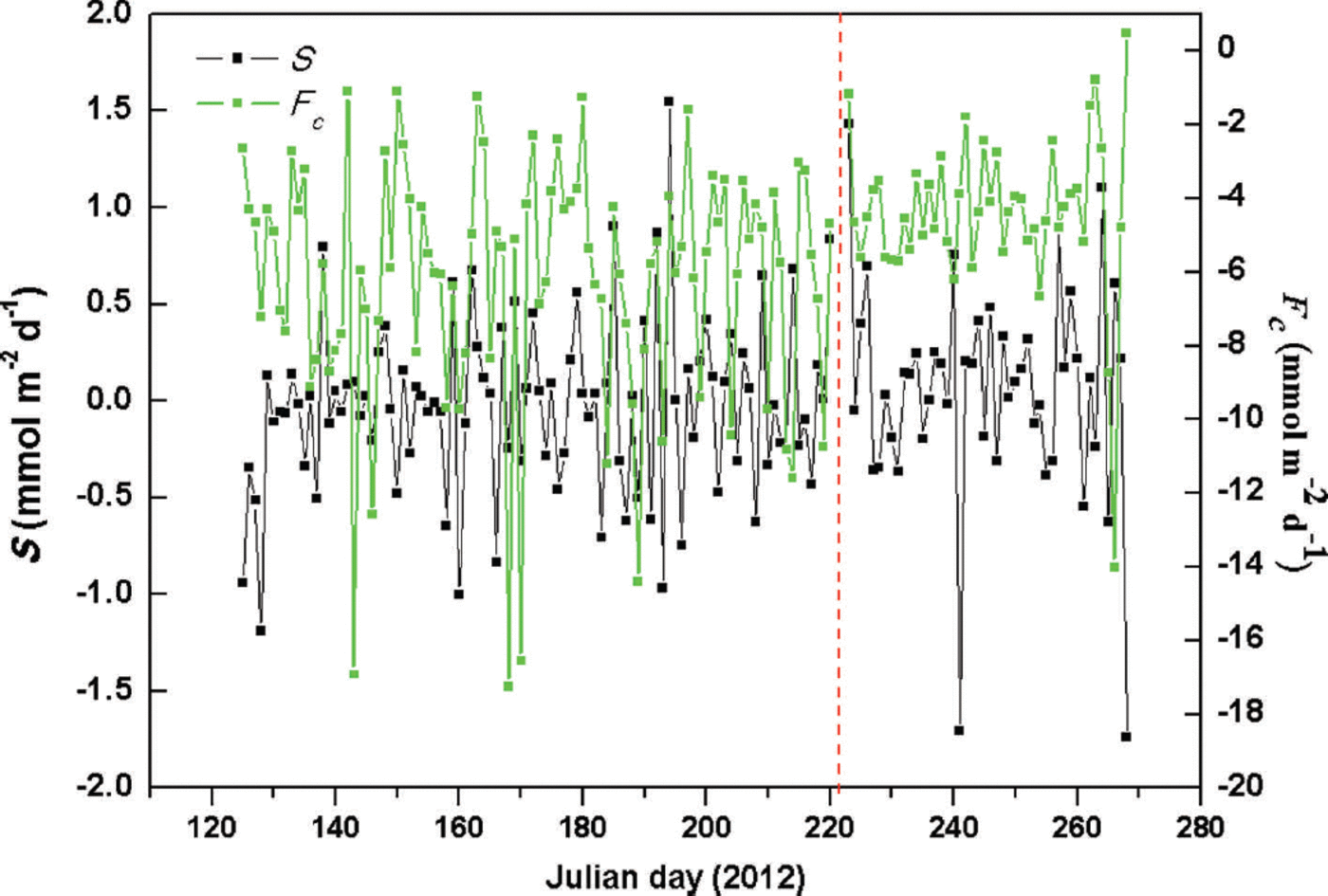
Fig. 3. Study area variations of daily Fc and S at sites A and B (right and left sides of vertical dotted line, respectively).
NGE rates affected by ice-melt intensity (IMI)
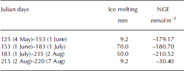
The most obvious characteristic of the NGE rate was that glacial meltwater was the fundamental carrier of carbonate and silicate hydrolysis but was not a determining factor in the daily NGE rates at site B (Fig. 4). Moreover, there were no significant changes in IMI, with daily NGE rates fluctuating around -6.26 mmol m–2 d–1 at that site (Table 1). For example, NGE rates at the site were -179.17 and -30.40 mmol m–2 between Julian days 125 (4 May) and 153 (1 June), and 215 (2 August) and 220 (7 August), respectively. The IMI was consistent across the same periods (Table 2). This suggests that the daily NGE rates are relatively stable with abundant soluble substances, and therefore not remarkably affected by IMI. At site A, however, there was correlation between IMI and NGE rates (Eqn (11)), while daily precipitation was <2 mm, demonstrating that the daily NGE rates, including those caused by the dissolution of carbonate and silicate, depended on ice melting. A mass of ice-melt water accelerated the strong chemical reactions, leading to a decrease in NGE rate:
where IMI is in mm and n is the number of days.
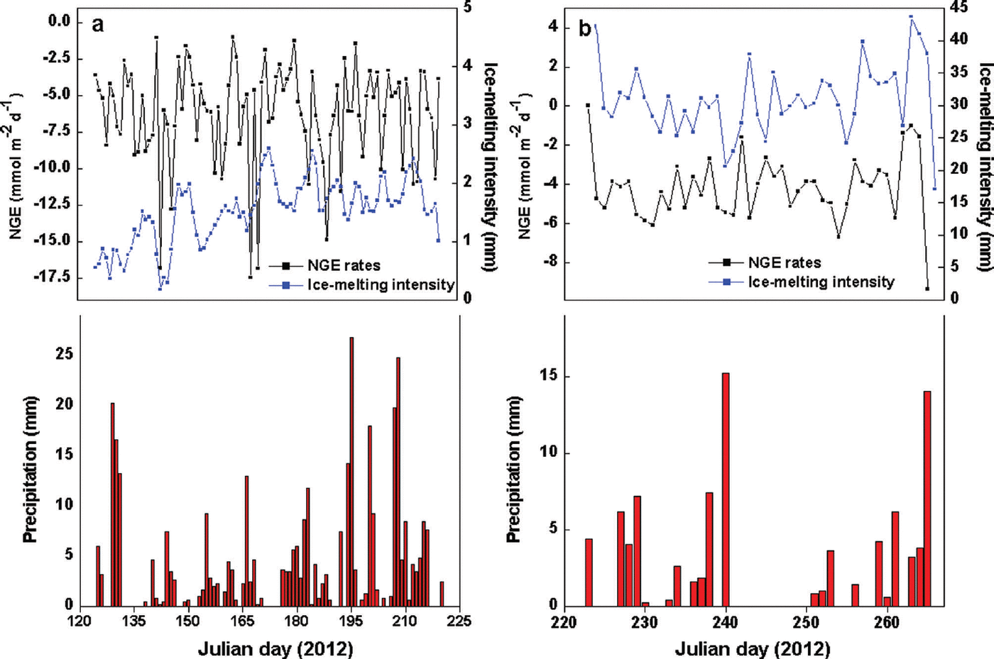
Fig. 4. Relationships of NGE rates, IMI and precipitation at (a) site B and (b) site A.
Table 2. Relationship between IMI and NGE rates at site B in 2012
Based on these results, it would not be possible to use the ice-melting and NGE rates to calculate the yearly flux of atmospheric CO2 consumption in the Koxkar glaciated region. To estimate the NGE rate for the whole glacial area, we used the degree-day model (Reference Singh, Kumar and AroraSingh and others, 2000; Reference Sicart, Hock and SixSicart and others, 2008; Reference MourshedMourshed, 2012; Reference Tennant, Menounos, Ainslie, Shea and JacksonTennant and others, 2012; Reference Mayr, Hagg, Mayer and BraunMayr and others, 2013) to calculate the IMI in the bare-ice region, and considered the characteristics of the NGE rate in the supraglacial debris region with the support of GIS, resulting in a daily NGE rate of about -1.23 ± 0.17 mmol m–2 d–1 between Julian days 125 (4 May) and 268 (24 September) in 2012. This estimate is less than the 1.84 mmol m–2 d–1 that was calculated in terms of ionic mass balance by Reference Wang, Xu, Zhang, Liu and HanWang and others (2010) in 2004, likely by ignoring the chemical reactions that follow glacier surface runoff in englacial conduit geometry. The NGE rate in the Koxkar glaciated area is greater than the CO2 drawdown of the Rhone and Oberaar glacial catchment in the Swiss Alps (Reference Hosein, Arn, Steinmann, Adatte and FöllmiHosein and others, 2004), and also higher than that of the Scottbreen glaciated basin in the Arctic (Reference Krawczyk and BartoszewskiKrawczyk and others, 2008). Substantial glacial debris might be the main reason for the higher chemical erosion and NGE rates in the Koxkar glacier area (Giles, 2002; Reference Hosein, Arn, Steinmann, Adatte and FöllmiHosein and others, 2004; Reference Krawczyk and BartoszewskiKrawczyk and others, 2008; Reference Zhang, Jin, Li, Yu and XiaoZhang and others, 2013).
Conclusions
At Koxkar glacier, atmospheric CO2 concentrations have gradually decreased as atmospheric temperatures have increased. The average values of hourly NGE were approximately –0.05 and –0.07 mmol m–2 s–1 for bare ice and supraglacial moraine, respectively. This implies that the basin is a sink for atmospheric CO2 above the glacial surface during melting seasons because of existing hydrochemical conditions and mineralogical reactions under ice-melting water. The CO2 storage (S) rates had little effect on NGE rates in the glaciated area, accounting for only 1.36% and 0.51% of the total NGE rate at sites A and B, respectively. A NGE rate was analyzed in the glacier region. Using the degree-day model to calculate glacial ablation in a bare-ice region, and considering the characteristics of the NGE rate in a region of supraglacial debris with the support of GIS, the daily NGE rate was calculated as approximately -1.23±0.17mmolm–2d-1 between Julian days 125 and 268 in 2012. This could be lower than the actual value, because chemical reactions that follow the process of glacier surface runoff in englacial conduit geometry are not considered.
Acknowledgements
The work was supported by the China National Natural Science Foundation (grant Nos. 41001039, 41130638 and 41130641). We appreciate the comments of two anonymous reviewers.


 Open access