


I. INTRODUCTION
Most of the digital images we can see on the Internet are called low dynamic range (LDR) images. Their pixel values range from 0 to 255, and the ratio of max luminance to min luminance is 255, which may not reflect the real world exactly. High dynamic range (HDR) images provide a wider luminance range compared to LDR images, and they are closer to human visual system (HVS). Instead of conventional output devices, displaying HDR images requires high-bit-depth output devices. But for now, most existing output devices can only show LDR images. The general solution for this problem is to use a tone-mapping operator (TMO) that converts HDR to LDR images [Reference Reinhard, Stark, Shirley and Ferwerda1], thus any LDR device can display the tone mapped version of HDR images. HDR images can improve quality of experience in most of multimedia applications, such as photography, video, and 3D technology. But a primary drawback of HDR images is that memory and bandwidth requirements are significantly higher than conventional ones. So the compression method targeting for HDR images is in great need. For this reason, more and more researches have focused on this field.
Although some researchers are interested in HDR only compression schemes [Reference Koz and Dufaux2], the most popular image compression technique is still JPEG (ISO/IEC 10918). For most users, if they only have JPEG decoder on their devices, they will not know any information about the HDR content. As a result, an HDR image compression algorithm should provide JPEG compatibility to users only who have JPEG decoder. JPEG committee proposed JPEG XT standard (ISO/IEC 18477), which is a JPEG compatible HDR image compression scheme [Reference Artusi, Mantiuk, Richter and Korshunov3, Reference Richter, Artusi and Ebrahimi4]. The JPEG XT standard aims to provide higher bit depth support that can be seamlessly integrated into existing products and applications. While offering new features such as lossy or lossless representation of HDR images, JPEG XT remains backward compatible with the legacy JPEG standard. Therefore, legacy applications can reconstruct an 8-bit/sample LDR image from any JPEG XT code stream. The LDR version of the image and the original HDR image are related by a tone-mapping process that is not constrained by the standard and can be freely defined by the encoder. Although the JPEG XT standard promotes the development of HDR imaging technology and is widely accepted, still there is much room for improvements.
Khan [Reference Khan5] proposed a non-linear quantization algorithm aiming at reducing data volume of the extension layer. This method can significantly enhance the amount of details preserved in the extension layer, and therefore improve the encoding efficiency. It is also proved that the quantization algorithm can improve the performance on several existing two-layer encoding methods. Iwahashi et al. [Reference Iwahashi, Hamzah, Yoshida and Kiya6] used noise bias compensation to reduce variance of the noise. They defined noise bias as the mean of the noise in the same observed pixel value from different original values, and compensated it according to an observed pixel value. This method has positive effect on bit rate saving at low bit rate lossy compression of LDR images. Pendu et al. [Reference Pendu, Guillemot and Thoreau7] designed template-based inter layer prediction in order to perform the inverse tone mapping of a block without transmitting any additional parameter to the decoder. This method can improve accuracy of inverse tone-mapping model, thus obtained higher SSIM of reconstructed HDR images. Korshunov and Ebrahimi's work [Reference Korshunov and Ebrahimi8] is more interesting. They demonstrated no one tone-mapping algorithm can always stand out when compared with others. The choice of the best algorithm not only depends on the content, but also depends on the device used and other environmental parameters. They take all of those factors into consideration and optimize the performance. Fujiku et al. [Reference Fujiki, Adami, Jinno and Okuda9] first calculated a base map, which is a blurred version of the HDR image, and used it to generate the LDR image. Their method is suitable to preserve local contrast and has lower computational complexity. Choi et al. [Reference Choi, Kwon, Lee and Kim10] proposed a novel method that is completely different from others. They generated the residual data in the DCT domain. The encoder predicted the DCT coefficients of the input HDR image based on LDR image, then prediction coefficients and DCT domain residual are encoded. Because inverse DCT process is not required in encoding phase, their method is rather efficient.
Although all of these methods are effective in most situations, the HVS factor is not considered. The purpose of HDR is to improve the quality of user's visual experience and make multimedia content more consistent with HVS. This means that some information in the image may be insensitive to the human eyes, but many bits have been wasted in encoding the redundant imperceptible information. Therefore, we should make a compromise between the high quality of the salient areas and the degradation of the non-salient areas. Feng and Abhayaratne [Reference Feng and Abhayaratne11] propose an HDR saliency estimation model and apply the visual saliency to guide HDR image compression. However, their work focuses on the saliency estimation model and existing HDR codec is used as a Blackbox. In this paper, we focus on the compression of HDR image with the guidance of visual saliency and propose a visual saliency-based HDR image compression scheme. We analyze and discover the correlation between visual saliency and residual image in HDR image compression. We use the extracted saliency map of a tone mapped HDR image to guide extension layer encoding. The correlation between visual saliency and residual image is exploited to adaptively tune the quantization parameter according to saliency of image content. We incorporate the visual saliency guidance into the HDR image codec. This will ensure much higher image quality of regions that humans are most interested, and lower quality of other unimportant regions. Our contributions are summarized into the following three points:
(1) A visual saliency-based HDR image compression scheme is proposed, in which the saliency map of a tone mapped HDR image is used to guide extension layer encoding.
(2) The correlation between visual saliency and residual image in HDR image compression is analyzed and exploited, which is modeled to adaptively tune the quantization parameter according to saliency of image content.
(3) Extensive experimental results show that our method outperforms JPEG XT profile A, B, C and other state-of-the-art methods while offering JPEG compatibility meanwhile.
The rest of the paper is organized as follows: Section II illustrates background information of this paper. Section III introduces the proposed method in details. Experimental results are given in Section IV, we first analyze the effect of different saliency models and influence of quality range. Then we compare the proposed scheme with JPEG XT profile A, B, C and other state-of-the-art methods. Finally, discussions and conclusions are given in Section V.
II. PRELIMINARY
A) JPEG XT
In JPEG XT standard part 7, a backward compatible HDR image compression scheme is proposed [Reference Artusi, Mantiuk, Richter and Korshunov3]. It is able to encode images with bit depths higher than 8 bits per channel. The input HDR image $I$ is encoded into base layer $B$
 and residual layer $R$
 codestreams as shown in Fig. 1. Base layer $B$
 is the tone mapped version of input HDR image $I$
 , which can be compressed by the JPEG encoder, and the base layer codestream is constructed to provide JPEG backward compatibility. The residual layer codestream allows a residual layer decoder to reconstruct the original HDR image $I$
 starting from the base layer $B$
 . The coding tools of the overall JPEG XT infrastructure used to merge $B$
 and $R$
 together are then profile dependent. Since that, the two-layer JPEG compatible compression framework has received universal approval. The choice of TMO is open to users. JPEG XT does not define an encoder, but provides three schemes about how to reconstruct the HDR image, named profiles A, B, and C. The main differences between them is how to merge the base layer image and extension layer image.
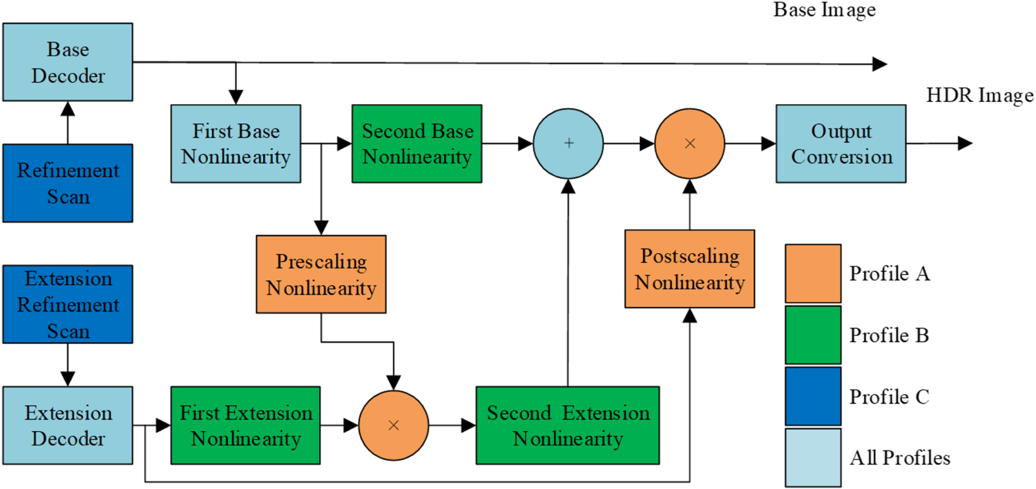
Fig. 1. Framework of JPEG XT.
Profile A reconstructs the HDR image $I$ by multiplying a luminance scale $\mu$
 with the base image $B$
 after inverse gamma correction using the first base non-linearity $\Phi _{A}$
 .
.

where $C$ and $D$
 are $3\times 3$
 matrices implementing color transformations, $\mu (\cdot )$
 is a scalar function of the luma component of the residual layer $R$
 , and $R^{\perp }$
 is the residual layer projected onto the chroma-subspace. The matrix $C$
 transforms from ITU-R BT.601 to the target colorspace in the residual layer. $D$
 is an inverse color decorrelation transformation from YCbCr to RGB in the residual layer to clearly separate the luminance component from the chromaticities at the encoding level. These matrices are also commonly used in the other two profiles. $S$
 is a row-vector transforming color into luminance, and $v(\cdot )$
 is a scalar function taking in input luminance values.
Profile B reconstructs the HDR image $I$ by computing the quotient that can be expressed as a difference in the logarithmic scale:

where $i$ is the index of the RGB color channels. $\Phi _B$
 and $\Psi _B$
 are two inverse gamma applied to the base and residual layers respectively. $\Phi _B$
 has the objective to linearize the base layer, while $\Psi _B$
 intends to better distribute values closer to zero in the residual layer. The scalar $\sigma$
 is an exposure parameter that scales the luminance of the output image to optimize the split between base and residual layers.
Profile C also employs a sum to merge base and residual images, but here $\Phi _C$ not only approximates an inverse gamma transformation, but implements a global inverse tone-mapping procedure that approximates the TMO that was used to create the LDR image. The residual layer $R$
 is encoded in the logarithmic domain directly, avoiding an additional transformation. Finally, log and exp are substituted by piecewise linear approximations that are implicitly defined by reinterpreting the bit-pattern of the half-logarithmic IEEE representation of floating-point numbers as integers. The reconstruction algorithm for profile C can then be written:

where $\hat {\Phi }_{C}(x) = \psi log(\Phi _C(x))$ , in which $\Phi _C$
 is the global inverse tone-mapping approximation. $2^{15}$
 is an offset shift to make the extension image symmetric around zero. The code stream never specifies $\Phi _C$
 directly, but rather includes a representation of $\hat {\Phi }_{C}$
 in the form of a lookup-table, allowing to skip the time-consuming computation of the logarithm.
B) Visual saliency
When watching at an image, human attention may be attracted by some specific regions, while other regions will be neglected. Visual saliency characterizes the most sensitive regions to HVS. In general, there are two categories of models to estimate the visual saliency of an image: bottom-up model and top-down model. In bottom-up model, saliency is only determined by how different a stimulus is from its surroundings. Top-down model, however, takes into account the internal state of the organism at this time [Reference Laurent, Christof and Ernst12]. Due to huge difficulty and dependency of prior knowledge, top-down model is less popular than bottom-up model. Here, we introduce some methods based on bottom-up model.
All of these models can be divided into global methods and local methods, or the combination of them. Cheng et al. [Reference Cheng, Zhang, Mitra, Huang and Hu13] proposed a global method base on histogram contrast. The saliency of a pixel is defined using its color contrast in Lab color space to all other pixels in the image. Hou et al. [Reference Hou and Zhang14] proposed a global method in log-spectrum domain. They calculated spectral residual of an image, and constructed the corresponding saliency map according to the spectral residual. Instead of global method, Achanta et al. [Reference Achanta, Estrada, Wils and S��sstrunk15] considered local method. In their opinions, saliency is determined as the local contrast of an image region with respect to its neighborhood at various scales. They added three saliency maps together, which is obtained in different scales, and got the final saliency. Goferman et al. [Reference Goferman, Zelnik-Manor and Tal16] combined both global and local methods. Their method considered local low-level features, i.e. contrast and color, and global features to get better result.
In recent years, saliency estimation of HDR image also has been considered [Reference Feng and Abhayaratne11, Reference Dong, Pourasad and Nasiopoulos17, Reference Xie, Jiang and Shao18, Reference Brémond, Petit and Tarel19]. Feng and Abhayaratne [Reference Feng and Abhayaratne11] propose an HDR saliency map detection method containing three parts: tone mapping, saliency detection, and saliency map fusion. Brémond et al. [Reference Brémond, Petit and Tarel19] proposes a Contrast-Feature algorithm to improve the saliency computation for HDR images. Due to wider luminance range, calculating saliency map of HDR image is more difficult. However, the principle does not change, some traditional methods are also available.
III. PROPOSED METHOD
A) Framework of our scheme
In this paper, we propose a JPEG compatible HDR image compression scheme based on visual saliency. The framework of our work is as shown in Fig. 2.
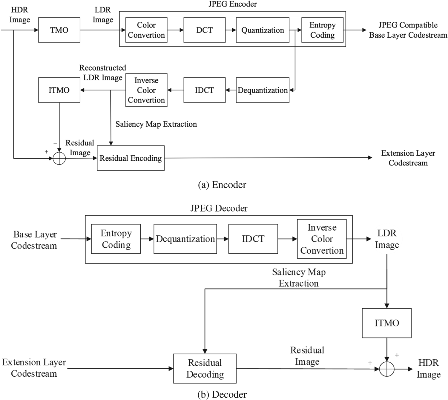
Fig. 2. Framework of our proposed method. (a) Encoder (b) Decoder.
In Fig. 2(a), the input HDR image is first tone mapped to get the corresponding LDR image. There are many previous works on tone mapping [Reference Rana, Valenzise and Dufaux20, Reference Rana, Valenzise and Dufaux21, Reference Rana, Singh and Valenzise22]. Rana et al. [Reference Rana, Valenzise and Dufaux20] and [Reference Rana, Valenzise and Dufaux21] propose a locally adaptive, image-matching optimal TMO which is guided by the support vector regressor (SVR) based predictor model. Rana et al. [Reference Rana, Singh and Valenzise22] propose a fast, parameter-free and scene-adaptable deep tone-mapping operator (DeepTMO) based on conditional generative adversarial network (cGAN). We need to point out that many existing tone-mapping methods can be applied in our compression framework, and more recent tone-mapping methods will lead higher performance. In order to focus on our compression scheme itself and make a fair comparison with existing compression methods, while considering the efficiency of the entire codec, we use a simple logarithmic function for tone mapping. Then the LDR image is encoded by JPEG (quality $q$ ) and sent to base layer codestream. The reconstructed LDR image, which is decoded by JPEG decoder, is used to encode the residual. The saliency map of reconstructed LDR is extracted by existing methods. Then all HDR values which are mapped to the same LDR value are averaged, and a look-up table is created for inverse TMO (ITMO). The ITMO of reconstructed LDR image is used to approximate the HDR image. Finally, the difference between original HDR image and approximated HDR image is called residual. In extension layer, we use another JPEG-based coding scheme (quality $Q$
 ), and adaptively set different $Q$
 for different blocks. Instead of converting to YCbCr color space, we directly encoded the residual in RGB color space. As for decoding, as shown in Fig. 2(b), the base layer codestream provides JPEG compatibility, which can be decoded by JPEG decoder. Then, the saliency map of reconstructed LDR image is extracted to guide the extension layer decoding, which is just the same way as encoding. At last, the residual image and ITMO of the reconstructed LDR image are combined to obtain the final reconstructed HDR image.
B) Residual analysis
The residual image is defined as follows:\enlargethispage{-6pt}

where $I$ denotes the original HDR image, $TMO$
 and $ITMO$
 denote the tone-mapping operator and corresponding inverse TMO, $COM$
 and $DEC$
 denote JPEG compression and decompression. Residual mainly comes from many-to-one mapping in TMO and ITMO and/or quantization error in JPEG compression and decompression.
In this section, we first analyze the correlation between residual and saliency map. Before calculating saliency map, the reconstructed LDR image is first gamma corrected with $\gamma = 1/2.4$ . The saliency maps are extracted by four different methods [Reference Cheng, Zhang, Mitra, Huang and Hu13, Reference Hou and Zhang14, Reference Achanta, Estrada, Wils and S��sstrunk15, Reference Goferman, Zelnik-Manor and Tal16]. For those methods which can not obtain full resolution saliency map, bicubic interpolation is applied to extend the obtained saliency maps to full resolution. The saliency is normalized to 1 by equation (5):

where $Sal$ and $Sal'$
 denote saliency map before and after normalization respectively. The correlation coefficient between two matrixes is defined as:

where $A$ and $B$
 denote two matrices, and $\bar {A} = \sum \nolimits _m \sum \nolimits _n A_{mn}$
 , $\bar {B} = \sum \nolimits _m \sum \nolimits _n B_{mn}$
 .
.
We averaged correlation between saliency map and absolute value of residual in red, green, and blue channels. We changed base layer image quality $q$ . From Table 1 we can see that for most cases, the residual images have relatively high correlation with the saliency maps. We notice for some cases the correlation coefficients between them are not very high, the reasons are from the following three aspects after our study. The first reason is the saliency estimation method. We need to point out that all these saliency estimation methods are objective approximations of saliency mechanism of HVS, thus their results are more or less inconsistent with the groundtruth. These four saliency estimation models extract saliency maps based on different principles. From the results, the Achanta's method [Reference Achanta, Estrada, Wils and S��sstrunk15] has the highest average correlation. This model calculates the difference between the pixel value of a point and its neighboring pixels on different scales, and then superimposes this difference on different scales. For smaller regions, the difference between the pixel and its surrounding pixels on any scale can be detected, and its saliency is the sum of these three different scales. Larger image areas can only be detected at larger scales. So this model always highlights small areas. In HDR images, the reconstruction error of the bright area is often the highest, that is, the residual is the largest. The scale of the bright area is generally not large and rarely appears continuously. This fits the essence of the model and therefore has the highest correlation, thus we choose this model in our scheme. The Hou's method [Reference Hou and Zhang14] has the lowest average correlation because it considers the frequency domain characteristics. The essence of the residual error is the sum of losses in the mapping and compression process, which is not related to the frequency domain. On average, this model is not suitable to guide the compression of HDR images. The second reason is the compression quality. In general, the differences among correlation coefficients are not large when the same image is compressed with different quality, so the correlation coefficients are nearly the same for different compression quality. The exception is the correlation between the residuals of AtriumNight and the saliency maps obtained using Achanta's method [Reference Achanta, Estrada, Wils and S��sstrunk15]. They are very relevant on low-quality images. However, the correlation decreases significantly as the compression quality improves. One possible reason is that high-quality images retain more details, and these newly appeared details makes the relevant local image blocks in low-quality images no longer relevant. The third reason is the test images. There is vast difference among the content of different images, which show quite different features. We find that not all image residuals are correlated with saliency maps. For example, the correlation coefficients of Nave and Rend06 are low, which indicates that the residuals of the two images are not concentrated in the visually significant areas but in the insensitive areas. For Tree and Rosette, the average of their correlation coefficients exceed 0.35, even up to 0.5. This shows that these image residuals are very related to saliency, that is, the areas with large residuals are also the areas that the human eye are sensitive to. For most cases, we can draw this conclusion.
Table 1. Correlation between residual image and saliency map.

More intuitive results can be found in Figs 3 and 4. It is more obvious from Figs 3 and 4 that the residual layer and the saliency map are highly correlated. Specifically, the probability that the residual layer and the saliency map are “light” or “dark” at the same location is very high, which indicates that it is reasonable to use the saliency map to approximate the distribution of the residuals. For the decoder, although the distribution of the residuals cannot be obtained, it is possible to obtain a saliency map based on the reconstructed LDR image, thus obtaining the approximate distribution of the original residuals. Applying this property to compression will effectively guide the decoder to allocate the code stream more reasonably, and finally improve the overall quality of image compression.

Fig. 3. Visualization of residual layers and saliency maps from different methods for test images Memorial, AtriumNight, Tree, and Nave. For each row, the first image is the residual layer, the second to the fifth images are saliency map extracted by Cheng's method [Reference Cheng, Zhang, Mitra, Huang and Hu13], Hou's method [Reference Hou and Zhang14], Achanta's method [Reference Achanta, Estrada, Wils and S��sstrunk15], and Goferman's method [Reference Goferman, Zelnik-Manor and Tal16] respectively. (a) Memorial, (b) AtriumNight, (c) Tree, (d) Nave.

Fig. 4. Visualization of residual layers and saliency maps from different methods for test images Rosette, BigFogMap, Rend06, and Rend09. For each row, the first image is the residual layer, the second to the fifth images are saliency map extracted by Cheng's method [Reference Cheng, Zhang, Mitra, Huang and Hu13], Hou's method [Reference Hou and Zhang14], Achanta's method [Reference Achanta, Estrada, Wils and S��sstrunk15], and Goferman's method [Reference Goferman, Zelnik-Manor and Tal16] respectively. (a) Rosette, (b) BigFogMap, (c) Rend06, (d) Rend09.
C) Adaptive quality parameter
As we can see in Section III B), there exists correlation between residual and saliency map. As a result, we can use visual saliency to guide residual layer coding.
In JPEG coding, an image is divided into $8\times 8$ blocks, thus we also can segment the saliency map in the same way. We first normalize the saliency map by equation (5). Then we sum up the saliency of each block, calculating the mean saliency $\bar {S}$
 of all blocks. We specify the baseline quality of extension layer $Q$
 , but it is just an “average” quality of all the blocks. For the blocks whose saliency are greater than $\bar {S}$
 , their quality is much higher, otherwise, the quality is lower. Equation (7) shows the relationship between them:

where $s$ denotes the saliency of current block, and $k$
 is the parameter to control range between the maximum and minimum of the quality. $dQ$
 is “relative quality” of current block. As a result, the quality of current block is:

In order to avoid negative quality for the least salient region, we set minimal $dQ$ to $-Q/2$
 . The relative quality calculated by (8) is adjusted to $100$
 if it is greater than $100$
 . Equation (9) shows the final quality of each block.

As a result, quantization level is adaptively selected according to saliency. Thus the rate-distortion performance of extension layer coding can be optimized. Take Fig. 5 as an example, in this case, baseline quality $Q$ is $70$
 and $k$
 is$0.4$
 . Using equation (5), we can get the highest quality $77$
 and the lowest quality $46$
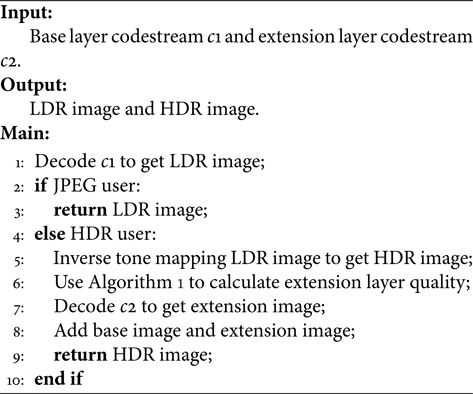
 . The whole process is as depicted in Algorithm 1. Our proposed visual saliency-based HDR image compression and decompression are as in Algorithms 2 and 3 respectively.

Fig. 5. Example of extension layer quality distribution matrix. (a) Reconstructed LDR image, (b) Saliency map, (c) Extension layer quality distribution.
Algorithm 1. Extension layer quality calculation

Algorithm 2. Compression algorithm

Algorithm 3. Decompression algorithm

IV. EXPERIMENTAL RESULTS
A) Experimental setup
In this section, extensive experiments are carried out to validate the performance of our compression scheme. We implement our proposed method in PC with Window 10 and MATLAB 2016b. The eight test images are from Ward's HDR image set [23], as shown in Fig. 6, with their details shown in Table 2.

Fig. 6. Test image set.
Table 2. Details of test images.

HDR visible difference predictor 2 (HDR-VDP-2) is adopted as evaluation metric as it is most consistent with human eyes [Reference Mantiuk, Kim, Rempel and Heidrich24]. As the most widely used method to estimate HDR image quality, it can predict similarity between a pair of images and calculate mean-opinion-score of test images.
B) Quality range adjusting
As mentioned in Section III B), $k$ is the parameter to control the range of quality. In this section, we evaluate the influence of different $k$
 . Test image Memorial and Achanta's saliency detection method [Reference Achanta, Estrada, Wils and S��sstrunk15] is used. Then, we set base layer image quality $q$
 equal to extension layer quality $Q$
 . The result is shown in Fig. 7.

Fig. 7. Different quality ranges.
The result shows that: (1) Adaptive quality parameter is better than fix quality. $k = 0$ means $Q$
 is equal to all blocks. It is obvious that setting quality adaptively has positive effect. (2) At low bit rate, $k\neq 0$
 has almost the same performance as $k = 0$
 . Because the baseline $Q$
 itself is small, the quality of non-salient region is extremely small, probably discarding all residual information. When the bit rate increases, all the blocks can obtain a suitable quality. (3) As $k$
 increases, the quality distribution become more and more uneven. In this case, when the quality is high, salient region can be nearly lossless coded. However, quality of other regions is not so satisfactory. Generally, set a moderate $k$
 can optimize the performance.
C) Bitstream balancing
In this paper, bitstream balance refers to the bitrate allocation between the base layer and the extension layer when the total bitrate is fixed. In previous section, we balance the bitstream between salient and non-salient regions in the extension layer. In this section we discuss the allocation of bitstream between the base layer and the extension layer. The practical significance of this discussion is that when the user's storage or bandwidth are limited to a fixed bit rate $C$ , it is important to distribute these bitstreams to the base layer and the extension layer to achieve best quality of reconstructed HDR image.
In the following experiments, we fixed the total bit rate at 2, 3, and 4 bpp respectively. As shown in Fig. 8, we can draw these conclusions from the experimental results: (1) A moderate distribution can get the best result, over-allocating on either base layer or extension layer is not always good. (2) With the increase of bitstream, the optimal point moves to the right, which means base layer tends to occupy more bitstream. (3) The gap between optimal point and other points shrinks rapidly when the bitstream is sufficient. That means bitstream balance is quite a problem at low bit rate. However, as the total bitstream is enough, allocating the bitstream between base layer and extension layer has little effect on overall performance.

Fig. 8. Bitstream balancing.
D) Comparison with JPEG XT and other methods
To validate the efficiency of our proposed method, we make extensive comparison with other methods. As mentioned in Section II A), we do not take JPEG XT profile D into consideration, so we compare our method with profiles A, B, C. They are implemented by JPEG XT working group [25], and the recommended parameters are used in our experiments. Besides that, we compare our method with other state-of-the-art work, such as Choi et al. [Reference Choi, Kwon, Lee and Kim10], Wei et al. [Reference Wei, Wen and Li26], and Feyiz et al. [Reference Feyiz, Kamisli and Zerman27]. HDR-VDP-2 [Reference Mantiuk, Kim, Rempel and Heidrich24] and SSIM [Reference Wang, Bovik and Sheikh28] are adopted as the evaluation metric of objective quality. In our proposed method, Achanta's saliency map is applied due to its highest correlation to residual image, and the parameter is set as $k = 0.3$ . The objective quality comparison results are as shown in Figs 9 and 10.

Fig. 9. HDR-VDP-2 results comparison with different methods.

Fig. 10. SSIM results comparison with different methods.
In general, our method outperforms all of other methods, except for low bit rates. One possible reason is that the baseline quality $Q$ is not so high when the bit rate is low, which may cause severe degradation in non-salient region. As a result, the total HDR-VDP-2 of whole image is inferior to JPEG XT. However, when the bit rate increases, the balance between salient regions and non-salient ones is desirable. So our proposed method is better than other methods when the bit rate is sufficient.
We also compare the subjective quality at a fix bit rate, as shown in Figs 11, 12 and 13. For clarity of comparison, the decoded image is zoomed in specified region ($100 \times 100$ pixels). The regions in red square are salient regions and regions in blue square are non-salient ones. As we can see, in salient regions, our method achieves best quality. While in non-salient region, our method is comparable to JPEG XT profiles A, B, and slightly inferior to profile C.

Fig. 11. Visual quality comparison of memorial with different methods at 3.2 bpp. (On the left is the original image, top two rows on the right are non-salient regions of reconstructed image, and two bottom rows on the right are salient ones. From left to right, the first row is original image, official implementation of JPEG XT profile A,B,C, the second row is Choi's method10 [Reference Choi, Kwon, Lee and Kim10], Wei's method21 [Reference Rana, Valenzise and Dufaux21], Feyiz's method22 [Reference Rana, Singh and Valenzise22], and our proposed method, respectively.)

Fig. 12. Visual quality comparison of AtriumNight with different methods at 2.0 bpp. (On the left is the original image, top two rows on the right are non-salient regions of reconstructed image, and two bottom rows on the right are salient ones. From left to right, the first row is original image, official implementation of JPEG XT profile A,B,C, the second row is Choi's method10 [Reference Choi, Kwon, Lee and Kim10], Wei's method 21 [Reference Rana, Valenzise and Dufaux21], Feyiz's method 22 [Reference Rana, Singh and Valenzise22], and our proposed method, respectively.)

Fig. 13. Visual quality comparison of BigFogMap with different methods at 2.7 bpp. (On the left is the original image, top two rows on the right are non-salient regions of reconstructed image, and two bottom rows on the right are salient ones. From left to right, the first row is original image, official implementation of JPEG XT profile A,B,C, the second row is Choi's method [Reference Choi, Kwon, Lee and Kim10], Wei's method [Reference Wei, Wen and Li26], Feyiz's method [Reference Feyiz, Kamisli and Zerman27], and our proposed method, respectively.)
V. CONCLUSIONS
In this paper, a visual saliency-based HDR image compression scheme is proposed. It divides the input HDR image into two layers, base layer and extension layer. The base layer codestream provides JPEG backward compatibility, and any JPEG decoder can reconstruct LDR version of HDR image. Extension layer codestream helps to reconstruct the original HDR image. The saliency map of tone mapped HDR image is first extracted, then is used to guide extension layer coding. For the most salient region, we set the highest quality, and the quality of other regions is adaptively adjusted depending on its saliency.
Extensive experiments have been conducted to validate the proposed scheme. We analyze the correlation between residual image and saliency map extracted by some classical approaches. It can be easily proved that local model visual saliency will get better result. We also analyze the influence of quality range. Experimental result shows that a moderate parameter can control the quality range well. Then, we use them to guide extension layer compression, and compare it with JPEG XT profiles A, B, C. Using HDR-VDP-2 as evaluation metric, our method outperforms JPEG XT standard in both objective and subjective quality. The main reason is that our method balances the bit rate between salient regions and non-salient ones. This is a desirable trade-off to ensure higher quality of information that is significant to human eyes, and lower quality of redundant imperceptible information.
As to the running time, our proposed method is slower than JPEG XT, because saliency map and relative quality need to be calculated in both encoder and decoder side. The computational complexity of calculating saliency map is scheme dependent, while relative quality is easily computed. So in practice, a simple saliency extraction algorithm can keep the running time almost the same as JPEG XT.
ACKNOWLEDGMENT
This work is supported by the National Natural Science Foundation of China (No. 61906008, 61632006, 61672066, 61976011, 61671070), Scientific Research Project of Beijing Educational Committee (KM202010005013), and the Opening Project of Beijing Key Laboratory of Internet Culture and Digital Dissemination Research.
Jin Wang received the B.S. degree in computer science from Huazhong University of Science and Technology(HUST), Wuhan, China in 2006 and the M.S. and the Ph.D. degrees in computer science from Beijing University of Technology(BJUT), Beijing, China in 2010 and 2015, respectively. He is currently a lecturer in the Faculty of Information Technology at BJUT. His areas of interests include digital image processing, image/video compression and computer vision.
Shenda Li received the M.S. degree in software engineering from Beijing University of Technology, Beijing, China, in 2019. His research interests is image compression and HDR image processing.
Qing Zhu received the M.S. and the Ph.D. degrees in electronic information and communication from Waseda University in 1994 and 2000 respectively. After graduation, she worked in the Institute of Information and Communication of Waseda University. She is currently a Professor with the Faculty of Information Technology, Beijing University of Technology. Her research interests include multimedia information processing technology, virtual reality technology and information integration technology.


 Open access