


1. Introduction
A gravity current (GC) is a generic name for the flow of a body of fluid of density  $\rho _0 + \Delta \rho$ embedded in a large domain of ambient fluid of density $\rho _0$, over a horizontal bottom. The flow is driven by the buoyancy $\Delta \rho g$ counteracted by inertial or viscous effects, where $g$ is the gravity acceleration. The density excess $\Delta \rho$ is due to the composition (e.g. salinity or temperature difference) with the ambient or the presence of small dispersed particles (particle-driven GC). In the classical problem, $\Delta \rho$ is prescribed explicitly in an initial reservoir (the lock-release problem) or by a supplying source. Various geometries and ranges of parameters have been investigated by experiments, simulations and approximate models (see Ungarish (Reference Ungarish2020) and the references therein). GCs sustained by a constant source are of great relevance to environmental and geophysical application (see Chowdhury & Testik Reference Chowdhury and Testik2014; Zhang & Hu Reference Zhang and Hu2022), and a particular problem is the effect of a moving source. The moving source introduces a competition between the buoyancy-induced motion and that of the homogeneous ambient; the most obvious effect of a moving source is the emergence of a non-symmetric behaviour of the front of the buoyant fluid, which may be either co- or anti-flowing with respect to the ambient, and even fully arrested. This effect is well demonstrated, both experimentally and analytically, by Hogg, Hallworth & Huppert (Reference Hogg, Hallworth and Huppert2005) (referred to as HHH) in a configuration with a source at the top; see figure 1. The concept of a moving source also covers the situation of a fixed source in a moving ambient, which is relevant to discharge of pollutants within a river, and advection of downdraughts of cold air by the background wind.

Figure 1. Sketch of moving source at top flow field of HHH: (a) side view, and (b) front view. The velocities  $u_1,u_2$ of the dense-fluid currents and $U_s$ of the ambient fluid are in the system attached to the source. The heights of the currents are $h_1$ and $h_2$. The $\pm x$ domain is unbounded.
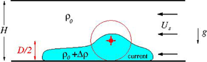
Ouillon et al. (Reference Ouillon, Kakoutas, Meiburg and Peacock2021) (hereafter OKMP) introduced a novel GC configuration (see figure 2): in a large ambient fluid of density  $\rho _0$ over a horizontal bottom, there is a ‘source of buoyancy’ that moves with constant speed $U_s$ parallel to the bottom in direction $-x$; the source effect is distributed in a virtual (non-disturbing) sphere of diameter $D$ whose centre is at height $D/2$ above the bottom. This is an idealization of the discharge unit of a sea-mining collector vehicle that travels along the seabed, resuspending the first few centimetres of the bed and continuously releasing a buoyant flux (see OKMP); constant $U_s$ and rate of discharge are plausible operational conditions that we carry over to the model. The fluid in the locus affected by the source gains density excess $\Delta \rho$, and spreads over the bottom, with typical speed $U_b$. As usual, there is a vertical front $y_f(x,t)$ between the dense fluid (the GC) and the ambient. The objective is to predict the behaviour of the dense fluid, in particular the position and speed of the front, and the thickness $h$. The flow is very different from that studied by HHH, and a separate investigation is needed. The evident difficulties are as follows. (i) The evaluation of the density excess near the source $\Delta \rho$ is a part of the problem (in contrast to the classical compositional GC; the resemblance with the particle-driven GC is slightly relevant). (ii) The spread of the current is coupled with the motion of the source, hence the front interface between current, $y_f(x,t)$, lacks a predetermined shape – in contrast to two-dimensional (2-D) or axisymmetric classical currents.

Figure 2. Sketch of the moving source at bottom flow of OKMP in the  $xyz$ system attached to the centre of the source. Upper diagram: side view of $y=0$ plane. Lower diagrams: top view of front at some $t$ for cases(a) $a=0$, (b) subcritical $a< a_{crit}$, (c) supercritical wedge $a>a_{crit}$. The red circle represents the source influence sphere of diameter $D$. The $xy$ domain is unbounded.
OKMP used a Boussinesq code with high resolution for direct numerical simulations (DNS) of the flow in a Cartesian box domain. The bottom and the top (at height  $H=1.5D$) were solid no-slip boundaries, while the vertical boundaries were practically non-restrictive. The domain is initially (at time $t=0$) filled with stationary fluid (the ambient) of density $\rho _0$. The source of buoyancy is envisaged as a virtual sphere of diameter $D$ tangent to the bottom, whose centre moves with constant speed $U_s$ in the horizontal direction $-x$; see figure 2. The source increases the density (and hence the mass) of the system according to
 \begin{equation} \Delta \rho \times \mathcal{V}_c = ({\rm \pi}/6) \rho_0 S D^3 t, \end{equation}
where  $S$ is a given time constant, called ‘the intensity of the source’, and $t$ is the time. Equation (1.1) is a global mass-increase balance. The left-hand side of (1.1) represents the product of density excess and volume of larger density $\mathcal {V}_c(t)$ of the GC; $g \Delta \rho \mathcal {V}_c$ is the buoyancy addition to the system during time $t$. The distribution (propagation) of the dense fluid is the challenge of the study. By scaling analysis, OKMP concluded that the typical speed of propagation of the current is $U_b = (SgD^2)^{1/3}$, and that when the pertinent Reynolds ( $Re_b = U_b D/\nu$) and Péclet ( $Pe_b = Re_b\,Sc$) numbers are large, the only governing dimensionless parameter of the flow is $a = U_s/U_b$. Here, $\nu$ is the coefficient of viscosity, and $Sc$ is the Schmidt number. Ten simulations, for $0 \leqslant a\leqslant 2.52$ (at large $Re_b$ and $Pe_b$, with $Sc = 1$), were performed for long times ( $t \approx 60 D/U_b$) during which some clear-cut statistically averaged patterns of the GCs developed, as sketched in figures 2(a)–2(c). In particular, for $a> c_{crit} = 0.63$, the flow is in a ‘supercritical’ regime: the GC forms a wedge behind the source, and the lateral velocity $V_f$ of the front, upon some rescaling, tends to collapse on a universal steady-state dependency on $x$. OKMP present some experimental support to these novel simulation results, and discuss the possible practical use in deep-sea mining applications. Our concern here is the theoretical side of the flow field. The numerical simulation is an expensive and time-consuming tool; even a simple question like ‘what will change if the position of the top $H$ increases to $3D$?’ cannot be answered without weeks of work on a supercomputer. The novel problem is still intriguing. We must keep in mind that the driving source is an idealization of some unspecified mechanical device that adds mass with zero volume; e.g. this density increase can be achieved by release of very small solid particles, or by strong cooling (see Zhang & Hu Reference Zhang and Hu2022). The precise physical behaviour of the flow in the vicinity of the source is not specified, hence OKMP could report only qualitative agreement between their simulations and laboratory experiments. In this intriguing state of the problem, the effective investigation of various scenarios for the flow is of both academic and practical relevance. We argue that approximate analytical models are needed as an essential supporting tool for the progress of knowledge.
The need for an approximate model motivated the present work. The first attempt, reported here, is the adaptation of existing inertial–buoyancy models (see Huppert & Simpson Reference Huppert and Simpson1980; Ungarish Reference Ungarish2020) to the present system. Two convenient well-tested tools are: (i) the front-jump Froude formula  $Fr(h_f/H)$, where $h_f$ is the thickness of the front; and (ii) the box model. The extension to the present problem is not straightforward because, in contrast with the classical cases, the source does not supply the dense current, it just increases the density of the existing fluid; see (1.1). However, in the framework of some plausible assumptions, the combination of these tools is able to predict many of the salient patterns discerned by the more accurate simulations of OKMP, in particular the appearance of the supercritical regime and shape of the wedge. The model supports the scaling considerations and major dependency on the parameter $a$ elucidated by OKMP, and also points out the additional (albeit mild) dependency on $H$ that enters the process via the $Fr$ correlation. Box models should be used with care, and here we can benefit from the reliable support provided by the data of OKMP.
The structure of the paper is as follows. The formulation is given in § 2, and applied to  $U_s=0$ as a starting case of reference. Predictions of the model and comparisons with OKMP for $U_s > 0$ follow. The flow regimes and discriminator $a_{crit}$ are discussed in § 3.1. The subcritical regime is considered in § 3.2. Section 3.3 presents the solution of the supercritical wedge domain, and comparisons with OKMP. For contrast, the GC with source at top is considered briefly in § 4. Concluding remarks are given in § 5.
2. Formulation
For assembling a simplified model several assumptions and clarifications must be introduced. We employ the usual assumptions for the inertial–buoyancy GC: incompressible fluid, thin layer, sharp interface, negligible viscous forces, and Boussinesq. These are consistent with the study of OKMP. Our notation is consistent, but not identical, with OKMP; in particular, here  $(\Delta \rho /\rho _0)g$ is called the reduced gravity $g'$, while OKMP define this variable as the buoyancy $b$.
$b$.
The first key point is the behaviour of  $\Delta \rho$ (which is tantamount to that of $\Delta \rho /\rho _0$ and reduced gravity $g'$). The source generates an increase of global density according to (1.1). However, the local effect of the source is limited to the sphere $x^2+y^2+z^2 < D^2/4$. In this domain, there are large gradients that homogenize the local density; it is plausible that the initial formation is, roughly, a cylinder of height $D/2$ on the bottom, with dimensions $D/2$ in the $x$ and $y$ directions. We therefore assume that the outflux from that sphere is a constant $\Delta \rho$ (to be determined). Next, we assume that the dense fluid propagates as a distinct volume $\mathcal {V}_c$, enclosed by a sharp interface, with negligible mixing and entrainment. Thus after determining $\Delta \rho$, we can calculate $\mathcal {V}_c$ from (1.1). Furthermore, the mass-continuity equation now reads
 \begin{equation} \frac{\partial (\Delta \rho )}{\partial t} +{\boldsymbol{u}} \boldsymbol{\cdot} \boldsymbol{\nabla} (\Delta \rho) = 0 \quad (x^2+y^2+z^2 \geqslant D^2/4), \end{equation}
where  ${\boldsymbol {u}}$ is the velocity of the dense fluid in the $xyz$ system attached to the source. Since the initial condition is the constant $\Delta \rho$ on the boundary of the source-sphere, the solution of this equation by the method of characteristics is $\Delta \rho = {\rm const.}$ in the propagating GC. This also predicts a constant $g'$ for the GC. (Note that (2.9) of OKMP reduces to the present (2.1) outside the sphere of the source when $Pe_b \to \infty$.) We keep in mind that the value of $g'$ of the current (outside the source) is constant, but the value is not given. This is a difficulty of the problem.
The initially unknown  $g'$ prevents the simple determination of the appropriate scaling speed for the propagation of the current (e.g. $(g'D)^{1/2}$). Several candidates are available. First, and most certain, is the imposed $U_s$ of the source. Next, the length $D$ combined with (i) the gravity $g$ produces the wave-speed $U_w = (g D)^{1/2}$; and $D$ combined with (ii) source-intensity time $S$ yields the outflux speed $U_{out}= SD$. For scaling, OKMP introduced the ‘buoyancy speed’ defined by
 \begin{equation} U_b = (U_w^2 U_{out} )^{1/3} = (g S D^2)^{1/3}. \end{equation}
 The speed of the current needs a more complex estimate. The starting point (see Ungarish Reference Ungarish2020) is the jump condition formula for a front of height  $h_f$ between the fluid of density $\rho _0 + \Delta \rho$ and the ambient of density $\rho _0$, expressed as
 \begin{equation} u_f = Fr \left(\frac{h_f}{H}\right) \left ( \frac{\Delta \rho}{\rho_0}\,g h_f \right ) ^{1/2} = Fr \left(\frac{h_f}{H }\right) \left ( g' h_f \right ) ^{1/2}, \end{equation}
where, again,  $g' = (\Delta \rho /\rho _0)g$ is the reduced gravity. The essential point is that the jump of the front is relative to the embedding ambient fluid, as demonstrated by Shringarpure et al. (Reference Shringarpure, Lee, Ungarish and Balachandar2013), Chowdhury & Testik (Reference Chowdhury and Testik2014) and Hogg et al. (Reference Hogg, Nasr-Azadani, Ungarish and Meiburg2016). The $Fr$ coefficient for a Boussinesq system, as discussed here, is given conveniently by the semi-empirical Huppert–Simpson formula, as follows:
 \begin{equation} Fr =
Fr (\phi) = \left \{ \begin{array}{ll} \dfrac{1}{2}
\phi^{{-}1/3}, & \phi >0.075,
{\text{first branch}}, \\ 1.19, &
\phi \leqslant 0.075, {\text{second
branch}}, \end{array} \right.
\end{equation}
\begin{equation} Fr =
Fr (\phi) = \left \{ \begin{array}{ll} \dfrac{1}{2}
\phi^{{-}1/3}, & \phi >0.075,
{\text{first branch}}, \\ 1.19, &
\phi \leqslant 0.075, {\text{second
branch}}, \end{array} \right.
\end{equation}
where  $\phi = h_f/H$. Equation (2.3) predicts the speed of the front relative to the ambient in the direction normal to the front. This is a ‘local’ result that uses the properties of the flow in the vicinity of the jump. In practical systems, $\phi = h_f/H$ varies from 0 (a very deep current) to 0.5, approximately (the half-depth energy restriction elucidated by Benjamin Reference Benjamin1968). We therefore keep in mind that $Fr$ (see (2.4)) is expected to increase with $H$, but in general varies in the quite restricted range 0.63–1.19. In the system of OKMP, $H = 1.5 D$; we expect that the typical value for the GC is $h_f = D/2$, thus we obtain by (2.4) the typical $Fr = 0.72$.
We estimate  $u_f$ at early time, when the current is still close to the source, and the influence of $U_s$ is mild. We expect that the dense fluid first settles in a cylinder of height $h=D/2$ and diameter $D$ about the source (approximately), and spreads out for a while with constant $h_f = h = D/2$ and $u_f$. We argued above that $\Delta \rho$ is constant in this process. Using (1.1) we obtain the balance for the added mass rate of influx
 \begin{equation} {\rm \pi}\,\Delta \rho\,D^2 u_f /2 = ({\rm \pi}/6) \rho_0 SD^3. \end{equation}
We multiply by  $Fr^2\,g/\rho _0$, use (2.3), and rearrange as
 \begin{equation} u_f = \frac{1}{6^{1/3}}\,Fr^{2/3}\,(g SD^2)^{1/3} = \frac{1}{6^{1/3}}\,Fr^{2/3}\,U_b. \end{equation}
This result indicates that  $Fr$, i.e. the height ratio of current to ambient, enters into the behaviour of the flow field. Since we assume in this estimate $h_f = D/2$, the coefficient $(Fr^2/6)^{1/3}$ varies from $0.40$ for $H/D=1$ to 0.62 for $H/D \geqslant 6.7$. This implies that $U_b$ is a fair scale for the typical speed of propagation of the current created by the source. This justifies the scaling introduced by OKMP, and we will use it also here: in dimensionless variables, lengths are scaled with $D$, speed with $U_b$, and time with $D/U_b$.
For a given  $U_b$, we estimate the values of reduced density difference and reduced gravity by combining (2.3) for $h_f = D/2$ with (2.6), and obtain
 \begin{equation} g' = \frac{\Delta \rho}{\rho_0}\,g = \left ( \frac{2}{9} \right ) ^{1/3} \frac{1}{Fr ^{2/3} }\, \frac{U_b^2}{D} = \left ( \frac{2}{9} \right ) ^{1/3} \frac{1}{Fr ^{2/3} } \left ( \frac{S^2 D}{g} \right ) ^{1/3} g . \end{equation}
The Boussinesq approximation imposes the restriction  $\Delta \rho \ll \rho _0$ (or $g' \ll g$), which implies that the source acceleration $S^2 D$ is much smaller than $g$. In this estimate, we neglected the influence of $U_s$, and this will be reconsidered in § 3.3.
Following OKMP, we also introduce the dimensionless parameter
 \begin{equation} a = U_s/U_b. \end{equation}
Since our former estimates of flow-field variables depend of  $Fr$, we expect that the flow is governed by two parameters, $a$ and $Fr$. The range of $a$ is large, while that of $Fr$ is quite restricted to the range 0.63–1.19 (approximately), as explained above.
2.1. The  $U_s = 0$ case

This simple case (see figure 2a) is a convenient starting point for the box-model analysis. The flow is expected to be axisymmetric, hence we use a cylindrical coordinate system. We use dimensional variables unless stated otherwise.
We assume that the GC is a box of radius  $r_f(t)$ and height $h(t) = h_f(t)$, and constant $\Delta \rho$. Conservation of mass (1.1) gives
 \begin{equation} \frac{\Delta \rho}{\rho_0}\,{\rm \pi} r^2_f h = \frac{\rm \pi}{6}\,SD^3 t, \end{equation}
and the front condition (2.3) yields
 \begin{equation} u_f = \frac{{\rm d}r_f}{{\rm d}t} = Fr \left(g\,\frac{\Delta \rho}{\rho_0}\,h \right)^{1/2}. \end{equation}
For simplicity, we also assume a constant  $Fr$. In this case, the propagation (after some initial adjustment that is not of interest here) is of the form
 \begin{equation} r_f(t) = K t^\beta, \quad u_f = \beta Kt^{\beta -1}, \end{equation}
where  $K, \beta$ are constants. Substitution into (2.9)–(2.10) provides the result:
 $$\begin{gather} \beta = \tfrac{3}{4}, \end{gather}$$
 $$\begin{gather}K = \left ( \frac{8\,Fr^2}{27}\,g S D^3 \right ) ^{1/4} \text{(dimensional)}, \quad K = \left ( \frac{8\,Fr^2}{27} \right ) ^{1/4} \text{(dimensionless)}. \end{gather}$$
For  $Fr = 0.72$, the dimensionless variable is $K = 0.63$. We can compare the model prediction $r_f = 0.63 t^{3/4}$ with the simulation data. OKMP report that the DNS results for $a=0$ scale as $r_f \sim t^{3/4}$. By least-squares curve fit, they obtained $r_f \approx 0.44 t^{3/4}$ (dimensionless). This gives credence to the present model. Note that both the power $3/4$ and the prefactor $K$ were derived here analytically. The larger $K$ of the model can be attributed to the fact that the simulations use a no-slip bottom boundary, which is expected to reduce the speed of propagation.
Assume that at some  $t_1$, $r_f = D/2$ and $h_f = D/2$. Combining (2.10)–(2.12), we obtain
 \begin{equation} g' = \frac{\Delta \rho}{\rho_0}\,g = \frac{1}{2^{1/3}}\,\frac{1}{ Fr^{2/3}}\,\frac{U_b^2}{D} = \frac{1}{2^{1/3}}\, \frac{1}{ Fr^{2/3}} \left ( \frac{S^2 D}{g} \right ) ^{1/3} g . \end{equation}
 The present GC is like a constant-density compositional current of fixed  $\rho _c$ driven by a constant source (see Ungarish Reference Ungarish2020, § 8.2). Here, the density excess has been estimated, which introduces some uncertainty. The volume of the GC increases like $t$, while the thickness $h=h_f(t)$ decreases like $t^{-{1/2}}$ in the box-model approximation. In particular, we find that the effective Reynolds number $Re_e = u_f h (h/r_f)/\nu$ decreases like $t^{-2}$ or $r_f^{-8/3}$. In the OKMP simulation ‘Sim. 1’ ( $a=0$), $Re_b = 7937$, which can be considered as $Re_e$ at $r_f = 1/2$. An increase of $r_f$ to 5 thus yields $Re_e \approx Re_b \times 10^{-8/3} = 17$. This indicates that a significant part of the propagation $x_f(t)$ reported in figure 5 of OKMP is affected by viscous effects; this explains the smaller value of the fitted $K$.
$K$.
3. Predictions and comparisons for $U_s>0$

3.1. Flow regimes and $a_{crit}$

The patterns of figures 2(b) and 2(c) are elucidated by a simple superposition of the cylindrical solution (2.11a,b)–(2.12) with a stream  $U_s = a U_b$ towards the source. Using $r_f = Kt^{3/4}$ and $t= (r_f/K)^{4/3}$, we estimate the radius of maximum upstream spread $r_m$ at which an equilibrium of speeds appears, as follows:
 \begin{equation} (3/4) K t^{{-}1/4}_m = (3/4) K^{4/3} r_m^{{-}1/3} = U_s = a U_b. \end{equation}
The result, in dimensionless form, is
 \begin{equation} r_m = \frac{1}{\displaystyle a^3} \left ( \frac{3}{4} \right ) ^3K^4 = \frac{1}{\displaystyle a^3} \left ( \frac{3}{4} \right ) ^3 \frac{8\,Fr^2}{27} = \frac{1}{\displaystyle a^3}\,\frac{Fr^2}{8} \end{equation}
(see (2.12)), and the time for achieving this situation is
 \begin{equation} t_m = \frac{1}{\displaystyle a}\,\frac{3}{4}\,r_m = \frac{1}{\displaystyle a^4}\,\frac{3\,Fr^2}{32}. \end{equation}
 The major insight is that the upstream influence of the source is limited. The governing parameter is  $a$, while $Fr$ (i.e. the depth ratio $H/D$) plays a smaller role. We distinguish between two cases.
(i) The dense fluid spreads upstream for a while, then the foremost point of the front stops at a fixed distance from the source. This type is defined as the subcritical regime; see figure 2(b).
(ii) The domain of dense fluid is downstream. This type is defined as the supercritical regime; see figure 2(c).
The critical condition is attained when there is practically no upstream propagation from the source, i.e.  $r_m \approx 1/2$. From (3.2), we obtain
 \begin{equation} a_{crit} = Fr^{2/3}/2^{2/3}. \end{equation}
In general, this predicts a quite robust  $a_{crit}$ in the range 0.45–0.71 (because $Fr$ is in the range $0.63$– $1.19$). For $Fr = 0.72$ (relevant to OKMP), we obtain $a_{crit} = 0.51$. This is in fair agreement with the OKMP simulation result $0.63$. There are several reasons for the discrepancy. First, the present estimate is based on a crude superposition between two unperturbed flows (cylindrical outflow and constant opposing $U_s$ stream). In the real system, there is some interaction. The stopped current is expected to develop a thicker and more effective buoyancy front that is able to arrest a stronger stream (i.e. larger $a$). Second, viscous effects are expected to develop about the arrested front, reducing the impact of the opposing stream.
Our model predicts that  $a_{crit}$ increases with $Fr$, i.e. with $H$; see (2.4). This prediction cannot be compared with OKMP because no data for $H \ne 1.5D$ have been presented.
3.2. Subcritical regime
For small  $a$ (slow $U_s$), the leading point of the dense fluid may propagate a significant distance ahead of the source, and a long time is required until the maximum gap $x_m$ is attained. The prediction of (3.2) and (3.3) is displayed in figure 3. Here, $r_m$ is an estimate of the upstream distance ( $-x_m$ in the attached $xyz$ system) of penetration of the effect of the moving source in the subcritical regime, and $t_m$ estimates the time of formation of the quasi-steady blunt head that embeds the moving subcritical source; see figure 2(b).

Figure 3. Subcritical case: predicted (a) maximum upstream propagation distance  $x_m$ and (b) time $t_m$, as functions of $a$ for various $Fr$, in log–log plots.
The prediction is that  $-x_m$ increases like $a^{-3}$. Comparisons of (3.2) with figure 6 of OKMP (taking $Fr = 0.72$) show consistency of $-x_m$, as follows: for $a = 0.38$ and 0.25, the DNS values are 2.1 and 4.2, while the model gives 1.2 and 4.2, respectively. (The difference between 2.1 and 1.1 seems large, but we must keep in mind that when the arrested domain is close to the source, some local interactions may reduce the impact of $U_s$ and thus increase $x_m$. This has been discussed in the context of the DNS $a_{crit}$, which is larger than the prediction of the model. Taking this effect into consideration, we argue that when $|x_m| \approx 1$, an exaggeration of one unit is not so bad.) For the smaller $a=0.126$ shown in that figure of OKMP, the comparison is irrelevant. Since $t_m$ increases like $a^{-4}$ (see figure 3), the needed simulation time exceeds the range of the available data. For $a = 0.126$ and using $Fr = 0.72$, we obtain $t_m = 194$, while figure 6 of OKMP displays $t = 60$. Moreover, the influence of viscous effects may become dominant for the spreadout to $x_m$ expected for small $a$. These predictions are consistent with the observation of OKMP (p. 11) that it is ‘particularly challenging’ to simulate the asymptotic behaviour of the subcritical regime for small values of $a$.
$a$.
The model predicts that  $x_m$ and $t_m$ increase with $Fr$ (i.e. with the height of the ambient, $H$). There are no data for testing this prediction.
A more detailed prediction of the subcritical regime turns out to be a difficult task even in the framework of the box model. We leave this for future work and proceed to the other regime.
3.3. Supercritical regime
In this case (see figure 2c), the source propagates so fast that all the dense fluid is left behind, i.e. in  $x> 0$. The current is expected to form a wedge whose boundaries are $y = y_f(x,t)$. The objective is to calculate this domain. We use dimensional variables unless stated otherwise.
A new calculation of  $g'$ is needed, because the evaluation (2.13) has been obtained under the assumption that the density excess of the source spreads out quite freely ahead, behind and to the sides, and this cannot be valid for large $a$.
$a$.
For the supercritical regime we calculate  $g'$ as follows. We argue that the rapidly moving source, during a time interval $\Delta t$, leaves behind a cylinder of diameter $D$, length $U_s \Delta t$, and density excess $\Delta \rho$. The balance (1.1) is expressed as
 \begin{equation} \Delta \rho\,\frac{\rm \pi}{4}\,D^2 U_s\,\Delta t = \frac{\rm \pi}{6}\,\rho_0 SD^3\, \Delta t . \end{equation}
Multiplication with  $g$ and arrangement give
 \begin{equation} g' = g\, \frac{\Delta \rho}{\rho_0} = \frac{2}{3}\,\frac{S D}{U_s}\,g = \frac{2}{3}\,\frac{1}{\displaystyle a} \left (\frac{S^2 D}{g} \right ) ^{1/3}g . \end{equation}
 We argue that the dense fluid cylinder quickly collapses to a quasi-rectangular box on the bottom. Due to symmetry about  $y=0$, we consider only the $y>0$ half. The $yz$ cross-section has area $A_0 = ({\rm \pi} /8) D^2$, initial width $y_0 = D/2$, and initial height $h_0 = ({\rm \pi} /4)D$. Following OKMP, we assume that this rectangle generates a classical lock-release GC in the $y$ direction. The justification is that the $\partial (g' h) /\partial x$ gradient is expected to be small, hence the dominant propagation effect is in the lateral $y$ direction. A simple analytical solution can be obtained by the box-model approximation (Huppert & Simpson Reference Huppert and Simpson1980; Ungarish Reference Ungarish2020); see figure 4. For simplicity of notation, we define $Y = Y(x,\tau ) = y_f(x,\tau )$, where $\tau$ is the time from the instantaneous local lock-release.

Figure 4. Sketch of the box-model lateral propagation at fixed  $x_{G} = x- U_s \tau$, blue lines (the dashed line indicates initial $\tau =0$).
The box model assumes a homogeneous thickness  $h_f = h(\tau ) = A_0/Y$; we substitute this into the front condition (2.3). We obtain the speed of lateral propagation, in dimensional form:
 \begin{equation} V_f =
Fr \left(\frac{h}{H}\right) \sqrt{h}\sqrt{g'} = \left \{
\begin{array}{ll} \dfrac{1}{2} H^{1/3} A_0 ^{1/6}
\sqrt{g'}\, Y^{{-}1/6}, & \phi
>0.075, {\text{first branch}}, \\ 1.19 A_0
^{1/2} \sqrt{g'} \, Y^{{-}1/2}, & \phi
\leqslant 0.075, {\text{second branch}},
\end{array} \right.
\end{equation}
\begin{equation} V_f =
Fr \left(\frac{h}{H}\right) \sqrt{h}\sqrt{g'} = \left \{
\begin{array}{ll} \dfrac{1}{2} H^{1/3} A_0 ^{1/6}
\sqrt{g'}\, Y^{{-}1/6}, & \phi
>0.075, {\text{first branch}}, \\ 1.19 A_0
^{1/2} \sqrt{g'} \, Y^{{-}1/2}, & \phi
\leqslant 0.075, {\text{second branch}},
\end{array} \right.
\end{equation}
where  $\phi = A_0 / ( Y H)$, and we used the $Fr$ formula (2.4). The lateral propagation is calculated in a ground system $x_G,y_G,z_G$ attached to the bottom (see figure 2); the transformation to the $x,y,z$ attached to the source is $x_G = x-U_S \tau$ while $y_G = y, z_G=z$. For the fixed $x_G=0$, we integrate ${\rm d}Y/{\rm d}\tau = V_f$ subject to the initial condition $y_0$ at $\tau = 0$ and continuity at change of $Fr$ branches. During $\tau$, while the lateral front propagates to $Y(\tau )$, the plane $x_G=0$ becomes $x=U_s \tau$ in the source-attached system. This allows, at the end of integration, the substitution $\tau = x/U_s = x/(a U_b)$.
Finally, we switch to dimensionless variables:  $x,y,h,H$ scaled with $D$,
$D$,  $A_0$ scaled with $D^2$, $V_f$ scaled with $U_b$, and $g'$ scaled with $U_b^2/D = gSD/U_b$. We obtain, in the system attached to the source, the following curve. For the first branch (if relevant),
 \begin{equation} Y = \left ( C_1\,\frac{x}{a^{3/2}} + 2^{{-}7/6} \right ) ^{6/7}, \quad C_1 = \frac{7}{6^{3/2}} \left ( \frac{\rm \pi}{8} \right ) ^{1/6} H^{1/3}. \end{equation}
For the second branch,
 \begin{equation} Y = \left ( C_2\,\frac{x-x_2}{a^{3/2}} + Y_2^{3/2} \right ) ^{2/3}, \quad C_2 = 1.19 \left ( \frac{3{\rm \pi}}{16} \right ) ^{1/2}. \end{equation}
Here,  $x_2, Y_2$ are the values at the transition between the $Fr$ branches. If the initial GC is deep, $\phi = {\rm \pi}/(4 H) < 0.075$, then the motion is given by only the second branch with initial conditions $x_2 =0, Y_2 = 1/2$. When the first branch is relevant, the transition is given by $({\rm \pi} /8) /(Y_2 H) = 0.075$ or $Y_2 = 5.24 /H$, and the corresponding $x_2$ follows from (3.8a,b):
 \begin{equation} x_2 = ( Y_2^{7/6} - 2^{{-}7/6}) a ^{3/2} /C_1. \end{equation}
We obtained a closed prediction of the wedged-shaped GC. In the  $xyz$ system attached to the source, $y_f = Y$ is a steady function of $x$, in accord with OKMP. The slope ${\rm d} y_f/{{\rm d} x}$ is almost constant $\propto x^{-1/7}$ in the first branch, $\propto x^{-1/3}$ in the second branch. The thickness of the current $h = A_0/Y$ (see figure 6) decreases with $x$.
$x$.
With the known  $Y(x)$, we then calculate the lateral velocity of the front according to (3.7). In dimensionless form, this is expressed as
 \begin{equation} V_f
\sqrt{a} = \left \{ \begin{array}{lll}
\sqrt{\dfrac{2}{3}}\, \dfrac{1}{2}\,H^{1/3} \left (
\dfrac{\rm \pi}{8} \right ) ^{1/6} Y^{{-}1/6} = 0.35 H^{1/3}
Y^{{-}1/6}, & {\text{first branch}}, \\
\sqrt{\dfrac{2}{3}}\,1.19 \left ( \dfrac{\rm \pi}{8} \right )
^{1/2} Y^{{-}1/2}= 0.61 Y^{{-}1/2}, & {\text{second
branch}}. \end{array} \right.
\end{equation}
\begin{equation} V_f
\sqrt{a} = \left \{ \begin{array}{lll}
\sqrt{\dfrac{2}{3}}\, \dfrac{1}{2}\,H^{1/3} \left (
\dfrac{\rm \pi}{8} \right ) ^{1/6} Y^{{-}1/6} = 0.35 H^{1/3}
Y^{{-}1/6}, & {\text{first branch}}, \\
\sqrt{\dfrac{2}{3}}\,1.19 \left ( \dfrac{\rm \pi}{8} \right )
^{1/2} Y^{{-}1/2}= 0.61 Y^{{-}1/2}, & {\text{second
branch}}. \end{array} \right.
\end{equation}
In view of (3.8a,b)–(3.9a,b),  $Y^{1/6}$ and $Y^{1/2}$ change little with $x$. Therefore, the model predicts that the scaled $V_f \sqrt {a}$ is fairly constant (in particular on the first branch) for a fairly large range $x/a^{3/2}>1$. This is in accord with the observations of OKMP.
Figures 5 and 7 compare the predictions of the present model for the supercritical regime with the more rigorous results of OKMP, in dimensionless form. The model predicts correctly the shape of the wedge and the influence of the parameter  $a$. Quantitatively, the agreement for the small $a=0.63$ is not so good. This could be expected, because this case is on the border between subcritical and supercritical behaviours. There is also some discrepancy for small $x$. This can be attributed to the influence of the source: in the realistic system, there is an adjustment stage (with some oscillation) from the vertical collapse of the dense fluid ( $V_f = 0$) to the dominant lateral propagation. The approximate solution assumes an instantaneous dam-break motion.

Figure 5. Front position  $y_f$ in the frame attached to the source for various $a$. Model prediction (solid lines) and OKMP simulations (dash-dot lines).
The lateral speed is also predicted fairly well by the model. The simulation results  $V_f \sqrt {a}$ versus $x/a^{3/2}$ tend to collapse to a curve close to the theoretical blue line of figure 7. The discrepancy is larger for the small $a = 0.63$, and in general for $x < 3$, approximately. The reason is the influence of the source: the lateral motion is still in the phase of development from zero (as explained above), hence the model values for $x/a^{3/2} < 1$ are not displayed. This feature is quite well indicated by figure 6 (dimensionless). For small $a$ and $x<3$, there is a strong $\partial h/\partial x$ gradient, which means that the lateral motion is not dominant yet. This gradient also explains why the $V_f$ of the model (blue line) is below the results of the simulation in figure 7. In the realistic system, $\partial h/\partial x$ provides an addition to the driving force that carries the current away from the source.

Figure 6. Thickness of current  $h$ in frame attached to the source for various $a$ – model prediction.

Figure 7. Lateral front speed  $V_f\sqrt {a}$ in the frame attached to the source. Model prediction (solid line) and OKMP simulations (dash-dot lines).
The RLR line in figure 7 is a DNS result of a rectangular lock-release with  $y_0 = {\rm \pi}D/12$, $h_0 = D$ and $g' = U_b^2 /(a D)$. This GC contains the same mass of buoyant fluid $g' h_0 y_0$ as our box model. However, the initial speed is proportional to $g' h_0$, therefore the RLR line is above the blue line. Although the equations of motion of RLR are more accurate than the box model, the RLR results are not necessarily a more reliable physical description of the moving-source flow field. The initial and boundary conditions are certainly not fully compatible; it is difficult to justify how the source produces the initial column $h_0 = D$, $y_0 = ({\rm \pi} /12) D$, that has been used as the initial condition in the RLR results. There are no data for comparison with the thickness predictions of figure 6. The thickness of a GC is not a clear-cut result in numerical simulation, because in realistic systems, the interface is not sharp and contaminated by small instabilities oscillations. This renders a pointwise comparison of thickness quite inconclusive.
Finally, we note that the Boussinesq restriction  $g'/g \ll 1$ provided by (3.6) for the supercritical motion can be expressed as $SD \ll U_s$ or $S^2 D \ll g$. The latter coincides with the restriction derived for the subcritical cases.
4. Two-dimensional current by source at top
Hogg et al. (Reference Hogg, Hallworth and Huppert2005) (referred to as HHH) investigated the GC generated by a source of dense fluid moving at the top of the ambient fluid. We think that by briefly contrasting this case with the previous model, we can enhance our understanding of both problems.
The configuration of HHH is, essentially, as follows (see figure 1). A long rectangular tank of width  $W=26$ cm and height 50 cm is filled with water (the ambient fluid of density $\rho _0$) to height $H = 30$ cm. The source is a small nozzle (8 mm diameter) aligned vertically with the medial plane of the channel, with its end just below the free top water surface. The source (nozzle) moves with constant velocity $U_s$ with respect to the ground and the stagnant large body of water. The source releases a constant volume flux $Q$ of saline of known density $\rho _s \ (>\rho _0)$. The dense fluid, while sinking to the bottom, spreads out and entrains water. Upon reaching the bottom, two bottom GCs are formed: number 1 in the upstream direction, and number 2 in the downstream direction.
HHH performed 29 experiments with various  $Q$,
$Q$,  $\rho _s$, $U_s=0$ and $U_s = 2.9\ {\rm cm}\ {\rm s}^{-1}$. The GCs were in the Boussinesq buoyancy–inertial (large Reynolds number) regime. (For experimental convenience, the source was in a fixed position with respect to the tank, while the ambient fluid was set in motion relative to the source.) The propagation of the fronts was measured. The objective is a simple model for this propagation. Most of the analysis has been presented in HHH, and some of it will be repeated briefly here, with some small modifications and additions.
We define the source-flux per unit width  $q_s = Q/W$, the initial reduced gravity at the source $g'_s =(\rho _s/\rho _0 -1)g$, the buoyancy flux $B = q_s g'_s$, and the dilution coefficient $\psi = g'_c / g'_s$. Here, $g$ is the gravitational acceleration, and $g'_c$ is the reduced density of the current.
The analysis is performed in the system of coordinates  $xyz$ moving with the source; see figure 1. The fixed (ground) system is $x_G,y_G,z_G$ such that $x_G = x-U_st$, while $y_G=y$, $z_G=z$. The bottom and top of the ambient are at $z=0$ and $z=H$, respectively; the sidewalls are at $y=\pm W/2$. The velocity of interest is $u = u_G +U_s$ in the direction $x$. In the fixed system, the ambient fluid is motionless ( $u_{aG} = 0$), while in the source-system, the ambient moves with $u_a = U_s$.
Since  $W/2< H$, the dense plume from the source spreads out over the entire width of the tank before reaching the bottom. The modelling is facilitated by the expectation (supported by the experiments) that the GCs are 2-D (independent of the lateral coordinate $y$). The flux that hits the bottom splits into $\gamma q_s$ to the upstream and $(1-\gamma ) q_s$ to downstream, where $\gamma$ is expected to be a constant close to $0.5$. This produces two separated GCs, each one supplied by a constant source. The problem of a 2-D inertial GC sustained by a constant source is amenable to both the shallow-water and box-model solutions (see Ungarish (Reference Ungarish2020) and the references therein), and both methods yield the same results for the developed flow (at some distance from the source). In the present case, the theory predicts the formation of two currents, of constant height and speed $h_1, u_1$ and $h_2, u_2$, that carry the volume fluxes $h_1 |u_1|$ and $h_2 u_2$. The separated-currents assumption implies $u_1 <0$, $u_2>0$. The theory also indicates that for this problem, the appropriate scaling length is $h_b = (q_s^2/g'_s) ^{1/3}$ and the scaling speed is $U_b = B^{1/3}$. We introduce the dimensionless
 \begin{equation} a = U_s/U_b, \quad \tilde{H} = H/h_b. \end{equation}
We recall that in the OKMP problem, the scaling  $U_b$ was more ambiguous. The reason for the evident $U_b$ is that here the value of $g'_s$, and hence of the buoyancy flux $g'_s q_s$, is given.
The dilution is  $\psi$ in both currents. It is important to keep in mind that the dilution increases the volume of the initial flux, but does not affect the amount of dense material; in other words, the initial flux of buoyancy, $B$, is conserved.
We write the balance for the buoyancy fluxes (dimensional) as
 $$\begin{gather} |u_1|\,(h_1 \psi) g'_s = \gamma q_s g'_s = \gamma B, \end{gather}$$
 $$\begin{gather}u_2 (h_2 \psi) g'_s = (1-\gamma) q_s g'_s = (1-\gamma) B. \end{gather}$$
We recall that the reduced gravity of the currents is  $g'_c = \psi g'_s$. The front-jump conditions (2.3) yields
 \begin{equation} u_1 ={-}Fr_1\,(h_1 \psi g'_s)^{1/2} +U_s, \quad u_2 = Fr_2\,(h_2 \psi g'_s)^{1/2} + U_s. \end{equation}
 To obtain a useful solution, some closures are needed. First, we argue that for a fairly wide range of  $U_s$ (to be specified later), the flux that hits the bottom divides into equal parts, $\gamma = 1/2$, because the division region is fairly stagnant and governed by the local pressure. Second, we employ an empirical observation, taken from the analysis of HHH: assume $Fr_1=Fr_2 = Fr = 0.81$. Considering each current separately, we eliminate the $\psi h_i$ ( $i =1,2$) between the flux and the jump condition equations (4.2)–(4.4a,b).
We obtain, in dimensionless form, simple equations for the propagation of the currents:
 \begin{equation} |u_1|\,(|u_1| + a)^2 = Fr^2/2, \quad u_2 (u_2 - a)^2= Fr^2/2 . \end{equation}
For  $a=0$, this reduces to $-u_1= u_2 = Fr^{2/3}/2$.
The prediction (4.5a,b) is compared in figure 8 with the data of HHH. There is good qualitative agreement, and fair quantitative agreement. Interestingly, in spite of the significant entrainment during the descent of the plume from the top to bottom, the speeds of the dense GCs remain a robust function of the initial  $B$. Scaled with $U_b= B^{1/3}$, $u_1$ and $u_2$ depend only on the parameter $a = U_s/U_b$.

Figure 8. Speed of currents created by a moving top source, model (lines) and data (symbols), in the source-system, scaled with  $U_b = B^{1/3}$, versus $a=U_s/U_b$. (This is a modified version of figure 9 of HHH.)
In this context, we mention the investigation of Zhang & Hu (Reference Zhang and Hu2022) for a 2-D GC sustained by a source of buoyancy due to cooling in a semi-ellipse domain at  $x=0$. In this study, the source is not moving; the current at the bottom resembles the $a=0$ flow of HHH. Broadly, the scaling speed is also $B^{1/3}$ (with $g'_s$ due to cooling, not salinity), and the scaled velocity of the front is $\sim Fr^{2/3}$. The flow field has been simulated by a 2-D Boussinesq code. The moving-source extension is an interesting problem for future research.
Interestingly, in the model (4.5a,b), the propagation velocities are independent of the dilution. This makes the model relevant to a wide range of geometries and supply parameters. However, for further details, the value of  $\psi$ is needed, and this introduces a serious difficulty because the available model does not predict the dilution. HHH performed some relevant measurements that can be used for progress in understanding and method, but the quantitative results cannot be generalized.
The dilution measurements were performed by HHH for  $U_s =0$, and summarized in the curve-fit formula (recall that $\tilde {H} = (H/h_b)$)
 \begin{equation} \psi = [ 0.048 \tilde{H} + 6.8 ] ^{{-}1}. \end{equation}
The dilution occurs because of entrainment in the downward-plume motion. As long as the horizontal deviation of the plume due to  $U_s$ is small compared to $H$, the effect of $U_s$ is expected to be insignificant; this is the situation in the available experiments. Consequently, we assume that (4.6) is valid also for $U_s >0$. The correlation (4.6) is shown in figure 9.


The Reynolds numbers of the currents reflect the friction with the bottom of velocity  $u_B$ and are therefore estimated as $(u_{i} - u_B) h_i /\nu$ ( $i= 1,2$), where $\nu$ is the viscosity coefficient. In the experiments of HHH, there was no relative motion between the source and the bottom, i.e. $u_B =0$. Since $u_{i} h_i = 0.5 q_s/\psi$ (see (4.2)), we obtain $Re_1 = Re_2 = 0.5 q_s/(\nu \psi )$. The experimental values are in the range 600–2000. The dilution increases the thickness and thus reduces the shear in the current.
The foregoing results for the moving top-source have been reported by HHH. Here, we develop a criterion for the range of validity. We argue that when  $Re_1, Re_2$ are large, the validity of the model (4.5a,b) is bounded by classical energy restriction derived by Benjamin (Reference Benjamin1968) applied to the thicker GC: $h_1$ is at most the half-height of the ambient fluid. Consider the behaviour of the upstream GC. For a fixed geometry and source, the increase of $U_s$ tends to reduce $|u_1|$, and is expected to be counteracted by an increase of $h_1$ (in order to accommodate the flux $|u_1|\,h_1$). Suppose that $h_1$ (dimensionless) has reached the maximum $\tilde {H}/2$; further increase of $U_s$ will change the sign of $u_1$ in (4.4a,b), and invalidate the two-currents assumption. This yields, in dimensionless form,
 \begin{equation} a \leqslant a_{crit} = Fr \left [ \frac{1}{2}\,\psi \tilde{H} \right ]^{1/2} = Fr \left [ \frac{\tilde{H}}{2(0.048 \tilde{H}+ 6.8)} \right ]^{1/2}, \end{equation}
where (4.6) was used. In the experiments of HHH, the values of  $\tilde {H}$ were in the range 20–125, hence $a_{crit}$ according to (4.7) was in the range 1.0–1.7. Figure 9 shows the estimate (4.7) and the values of $a$ of the experimental data. (Recall that in the experiments, $U_s$ was fixed and $U_b = (q_s g'_s)^{1/3}$ varied.) The experiments, with one exception, were in the range $a < a_{crit}$. The exception is Exp. 26, for which $\tilde {H}=60.3$ and $a = a_{crit} = 1.43$. We conclude that only Exp. 26 was critical with respect to $a$, while for the other experiments, the model of two opposed currents is valid. Indeed, HHH do not display the value of $u_1$ for the critical Exp. 26, and we infer that it was close to zero or even slightly positive.
The theoretical justification for  $Fr = 0.81$ reported by HHH for both currents is lacking. We expect that the Huppert–Simpson correlation (2.4) is relevant. In all tested cases $h_1 > h_2$, which suggests $Fr_1 < Fr_2$. Some currents were deep, which suggests for $Fr_2$ a value close to 1.19. Our explanation of this discrepancy between theory and observations is as follows. First, there are uncertainties concerning the thickness of the nose of the currents that enters the $Fr$ formula. The source at $x = 0$ deviates from the idealized conditions of the inertial GC. Our model assumes $x$-independent $h_1$ and $h_2$, starting from $x=0$; therefore $h_1$ and $h_2$ must be regarded as some $x$-average in a more realistic system, not the exact values at the nose of the currents. Second, in general the downstream current 2 is longer than the counterpart 1. Therefore, current 2 is more influenced by the shear with the bottom and ambient, and by interfacial entrainment, and this reduces the speed of propagation. The measured value of $Fr_2$ contains the viscous influence, and is therefore smaller than expected. Due to the constant $Fr$ assumption, the model predicts that propagation of the currents is independent of the height of the ambient fluid. This conclusion must be used with care, because, as mentioned above, the constant $Fr = 0.81$ lacks justification in general.
Figures 8 and 9 confirm the relevance of the scaling used by this analysis and the fair accuracy of the simple two-currents model. The major deficiency is the restriction of the speed of the source to the subcritical  $a = U_s/U_b \leqslant a_{crit}$. Moreover, the calculation of $a_{crit}$ uses an empirical correlation for the dilution $\psi$. To our knowledge, the supercritical case, $a> a_{crit}$, has not been investigated. HHH have also considered the sustained flow of a particle-laden suspensions, which is outside the scope of the present discussion.
The comparison of the moving-source GCs configurations of HHH and OKMP reveals some similarities, but mostly very significant differences. Formally, both problems are governed by the parameter  $a= U_s/U_b$, but the reference speed $U_b$ is determined by different formulas. This is reflected by the very different values of $a_{crit}$ (about 1.5 and 0.5 for HHH and OKMP, respectively). Evidently, the model of HHH cannot be used for the flow studied by OKMP.
5. Concluding remarks
The GC created by a moving source of buoyancy close to the bottom is a novel problem that poses various difficulties of formulation and interpretation. The major available knowledge is provided by the analysis of heavy numerical simulation of a Boussinesq system on a supercomputer by OKMP. Here, we presented a simple box-model approximation that is expected to assist in the understanding and early design of various applications related to this flow.
We contrasted the flow field of OKMP with that of a moving source at the top of a tank studied by HHH. In the latter case, the density (and hence the reduced gravity) of the supplied fluid is known, and the resulting GC is two-dimensional; this simplifies the analysis significantly. Nevertheless, we show that the simple model developed by HHH (and confirmed by comparison with experimental data) is valid only for subcritical speed of the source,  $a < a_{crit}$. Although the mechanism that governs $a_{crit}$ in this flow is quite well understood, the calculation of the value uses empirical information. (A possible remedy is the incorporation of a governing equation for the dilution in the plume from the source to the bottom, but this requires a separate investigation.) In contrast, the problem of OKMP is three-dimensional, and the density at the source is not specified. However, it turns out that the more complicated case is amenable to a model that is more effective, more explicit, covers mostly the more intriguing supercritical source speed (while also providing useful insights into the subcritical case), and does not rely on empirical data.
The model is self-contained: the predictions are not reliant on adjustable parameters. The results are expressed in explicit formulas. Our model confirms the scalings introduced by OKMP. The scaling speed  $U_b$ is a strange average of $[(\sqrt {gD})^2 SD]^{1/3}$ that turns out to be a fair estimate of the initial speed of propagation of the front, $u_f$. Our analysis provided a sharp estimate for the Boussinesq limitation: the internal acceleration in the source domain, $S^2 D$, should be much smaller than $g$; in the supercritical case, this also implies that the speed in the source domain, $SD$, is much smaller than $U_s$. If these conditions are violated (which must be taken into account with realistic mechanical pumps), then the resulting GC may be non-Boussinesq and incompatible with the present model.
OKMP detected the dependency on one parameter, the speed ratio  $a=U_s/U_b$. The model confirms this dependency, but also indicates dependency on the value of the front-jump Froude number $Fr$. The convenient Huppert–Simpson formula translates this into a dependency on the height of the ambient fluid. The model predicts fairly well (compared with OKMP) the axisymmetric propagation for $a=0$, and that, upon increase of $a$, the upstream propagation is arrested at a distance $x_m \propto a^{-3}$ after a time period $t_m \propto a^{-4}$; for $a > a_{crit}$ (the supercritical regime), the entire GC propagates downstream as a wedge.
The model detected dependency also on the height of the ambient,  $H/D$, via the correlation for $Fr$. The model predicts that an increase of the height of the ambient, $H$, will cause an increase of $Fr$, and this is expected to cause an increase of $a_{crit}$, $x_m$, $t_m$ and $V_f$. In the subcritical regime, the increase of $Fr$ causes a decrease of $g'$, but in the supercritical regime, $g'$ is independent of $Fr$. The practical range of $Fr$ is 0.63–1.19, hence the influence of this parameter is not dramatic, but still sufficiently significant for experiments and applications. For example, $a_{crit}$ is expected to change (increase) by 53 % with $Fr$ in that range. The simulations of OKMP were mostly for one height of the ambient, $H/D = 1.5$, hence the variation of $Fr$ among the tested cases was small, and cannot be assessed from the available data.
Our model lacks rigour and an estimate of the error. However, this model certainly provides useful insights and simple approximations for the propagation for the novel moving-buoyancy-source GC system that is still in early stages of investigation. The box model is in general an unreliable tool, unless supported by a more accurate solution. In the present case, we benefit largely from support of the detailed simulations and data processing of OKMP. First, we note that our predictions concerning the influence of the parameter  $a$ are in full qualitative agreement with the results of OKMP, in particular the separation between subcritical and supercritical regimes at some value $a_{crit}$; in the supercritical regime, the buoyancy reduced gravity $g' \propto 1/a$, and the lateral speed $V_f \propto 1/\sqrt {a}$. Second, we found fair quantitative agreement concerning $a_{crit}$, the $K t ^{3/4}$ propagation for $a=0$, the steady shape $y_f(x)$ of the wedge (in the attached $xyz$ system), and the lateral speed $V_f$. Such agreement for a wide range of parameters is, in our opinion, an indication that the model captures well the governing mechanism of the flow. Considering the complexity of the full system (a simulation required ${\sim }48$ h on a 384 cores supercomputer), the performance of the analytical box model (without use of any adjustable parameter) is amazing. We expect that the use of the shallow-water equations can provide a more accurate formulation; however, the accuracy of the prediction depends on the precision of the initial conditions, and in this respect the uncertainties about the source of the present model remain.
In practical deep-sea mining collectors, the flow of the GC is prone to significant influence from effects that were not included in the present model, such as particle-driven buoyancy, non-quiescent ambient and a non-constant rate of supply. Such effects can be incorporated essentially in the box-model simplification (see Ungarish (Reference Ungarish2020, §§ 5.2, 10.2.3), and the references therein), but the details require a separate analysis. The present analysis can be used for providing some estimates about the importance of such effects, for example as follows.
The importance of particle sedimentation (typical speed  $W_p$) is represented by $\beta _p = W_p/U_s$, where $W_p = (2/9) (\rho _p/\rho _0 -1) g r_p^2/\nu$, $\rho _p$ and $r_p$ are the density and radius of the particles. When $\beta _p$ is small, the flow of the particle-driven GC is well approximated by the homogeneous GC with a corresponding fixed initial buoyancy (i.e. the dispersed particle are essential to the buoyancy, but the settling is negligible during the major propagation). In this case, the present model can be used. In practical cases, $\rho _p/\rho _0 -1 \approx 1.5$, hence the dominant variable is the particle size squared, $r_p^2$. For sufficiently small particles ( $r_p \leqslant 0.1$ mm, say) in water, and a typical $U_s =1 \ {\rm m}\ {\rm s}^{-1}$, we have $\beta _p < 3 \times 10^{-2}$.
Also, the non-quiescent ambient may be considered a perturbation of  $U_s$ (speed of the source with respect to the ambient) and hence a variation of the parameter $a$. The changing rate of supply may be interpreted as a change of the source intensity $S$. The solutions of the present model with appropriate changes of $a$ and $S$ are expected to provide some insights into the trends and magnitudes of these effects. The rapid results of the present model are beneficial in these estimates. Extensions of the present box model for these and other effects must be left for the future. We must keep in mind that the reliability of box-model solutions depends on the availability of a solid body of data for comparisons. We hope that future work on this problem will provide more data and insights that will enable the production and validation of improved models.
Declaration of interests
The author reports no conflict of interest.


 Open access