


Introduction
In nature, there are strong and tough biological materials that often possess remarkable hierarchical structures.Reference Meyers, Lin, Seki, Chen, Kad and Bodde1–Reference Vincent4 Examples of such natural materials include nacre, the exoskeleton of crustaceans, and spider webs. Using these examples, we emphasize the role of simple models for structures, which yield physical insights and often reveal useful scaling laws.
A scaling law gives an important physical quantity as a product of the powers of other physical parameters, as in Equations 1 and 2 given later in the text. Scaling laws are useful as guiding principles for various applications such as industrial development of reinforced materials, although they are mathematically exact only in the limit in which a number of physical parameters, X, Y, . . ., are much larger or smaller than certain values. Such a limit is often expressed as a set of inequalities, such as X >> X 0 and Y << Y 0.
In general, when a scaling law is obtained, its validity can be established through “data collapse.” A clear example is shown in Figure 1e: The original three scattered curves on the left fall onto a single curve on the right as a result of replotting the same data on new axes. The quantities used for the new x and y-axes are obtained by rescaling the quantities used for the original x and y axes in a way specified by the underlying scaling law shown in Figure 1e. (Figure 1d demonstrates another example of the data collapse.) Theoretically, scaling laws become exact only in a limit as stated previously. However, scaling laws are frequently valid in a practical sense over wide parameter ranges far beyond the theoretical restriction. Accordingly, scaling laws could be guiding principles for the development of various products in industries, such as new reinforced materials.
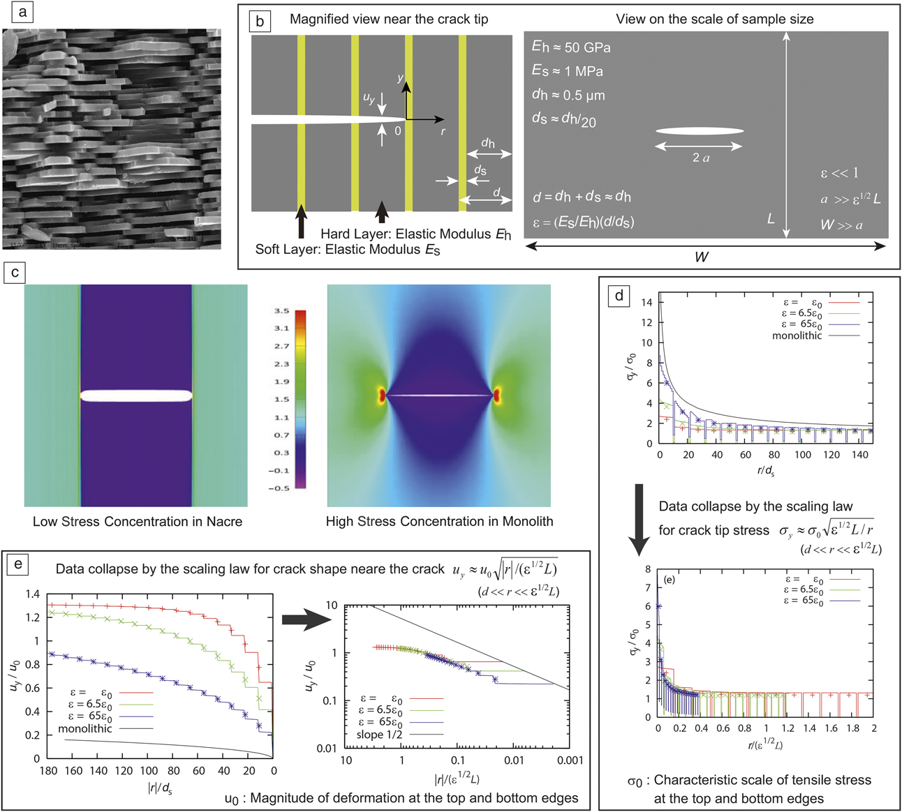
Figure 1. (a) Scanning electron microscope image of the section of nacre. The thickness of hard layers is approximately 0.5 µm. Because the soft layers are extremely thin (approximately 25 nm), they cannot be seen. (b) Illustration of a simplified model of nacre with a crack and structure parameters in the model. The left-hand illustration is drawn on the scale of layered structure, while the right-hand is drawn on the sample scale. (c) Stress distribution under the presence of a line crack in a plate of nacre (left) and a monolith of the hard element of nacre (right) with an intensity scale (middle), obtained by finite element calculations. Stress concentration near the crack tips is significantly reduced in nacre. (d) The top plot shows stress distribution around the right crack tip (b) of a horizontal line crack. Stress values are more reduced for smaller ε (the case ε = ε0 corresponds to real nacre). The bottom plot shows collapse of the same data by rescaling of the axes, confirming the validity of the scaling law shown in the panel. (e) Crack shape near the tip (left) and collapse of the data (right), confirming the scaling law shown in the panel. The plots show that the deformation is more enhanced for smaller ε0. (a) Courtesy of Prof. Dinesh Katti. (c–e) Created from data in Reference Reference Hamamoto and Okumura37.
To understand strength and/or toughness of materials for reinforcement, it is important to know the locations at which the stress field is locally enhanced when an external load is applied. Stress is concentrated at the tips of cracks or flaws, and such a concentrated tip stress can trigger failure of materials. Accordingly, it is indispensable to know how stress is concentrated, in particular when a simple line crack is present, as shown later in this article.
Nacre
Nacre is a strong biological material and possesses a magnificent hierarchical structure. It has been actively studiedReference Sarikaya, Liu and Aksay5–Reference Mayer8 together with, for example, bone,Reference Currey9–Reference Hellmich, Barthélémy and Dormieux11 and has inspired a number of artificial materials.Reference Kato12–Reference Corte and Leibler17 In nacre, the layered structure is composed of hard plates of aragonite and soft layers of proteinsReference Sarikaya, Liu and Aksay5 (see Figure 1a). Although soft layers are much thinner than hard layers, the fracture surface energy of nacre is a few thousand times as high as that of a monolith of hard aragonite.Reference Jackson, Vincent and Turner18 A number of different mechanisms for the toughness and strength of nacre have been pointed out on the basis of experimental observations: Soft layers are elongated in a stepwise way when stretched;Reference Smith, Schäffer, Viani, Thompson, Frederick, Kindt, Belcher, Stucky, Morse and Hansma19 thin compressive layers between hard layers lead to a remarkable strength;Reference Rao, Sanchez-Herencia, Beltz, McMeeking and Lange20 layer interfaces are rather rough;Reference Evans, Suo, Wang, Aksay, He and Hutchinson21 mineral bridges are found between layers;Reference Song, Soh and Bai22 and the surface of hard plates are wavy.Reference Barthelat, Tang, Zavattieri, Li and Espinosa23 Numerous theoretical studies have also been attempted, including studies using (1) elastic modelsReference Rao, Sanchez-Herencia, Beltz, McMeeking and Lange20 based on analytical solutionsReference Okumura and de Gennes24,Reference Okumura25 and scaling arguments,Reference de Gennes and Okumura26,Reference Okumura27 (2) viscoelastic models,Reference Okumura28 (3) micromechanical models,Reference Kotha, Li and Guzelsu29 and (4) numerical models such as finite-element models,Reference Barthelat, Tang, Zavattieri, Li and Espinosa23,Reference Katti, Katti, Sopp and Sarikaya30,Reference Ji and Gao31 a fuse network model,Reference Nukala, Zapperi and Šimunović32 and a model with a periodic Young’s modulus.Reference Fratzl, Gupta, Fischer and Kolednik33
The model discussed in Reference Reference Okumura and de Gennes24 is a simple layered structure of hard and soft plates, mimicking the structure of nacre as shown in Figure 1b. The model is based on the elastic moduli for soft and hard layers, E h and E s, respectively, and the thicknesses for soft and hard layers, d h and d s, respectively. These parameters satisfy the following relations: E h >> E s and d h >> d s. The elastic energy of this simple model can be constructed in the limit of small ε under the existence of a line crack perpendicular to the layers, where ε is defined as ε = (E s/E h)(d/d s) with d = d h + d s. Reasonable values of the parameters are d h = 0.5 µm, d s = d h/20, E h = 50 GPa, and E s = 1 MPa (the soft layers are like gelsReference Sumitomo, Kakisawa, Owaki and Kagawa34); for this set of parameters, ε is significantly small (ε ∼ 10−4). When the sample is stretched in the y direction, on the basis of the elastic energy in the small ε limit, the dominant component of deformation field u i and stress field σij are shown to be u y and σyy (termed σy in the following), with the other components being negligibly small in comparison.
In addition, the dominant component of the deformation field u y was shown to be governed by an anisotropic Laplace equation.Reference Okumura and de Gennes24 The equation for u y can be analytically solved under boundary conditions. For example, the conditions that describe a line crack of length 2a propagating in the r direction, as illustrated in Figure 1b,Reference Okumura and de Gennes24,Reference Hamamoto and Okumura35 are specified in the following way: The stress σy is zero at the surface of the crack (i.e., at y = 0 and −a < r < a), the deformation u y is zero at y = 0 from symmetry, except for the region −a < r < a in which the crack is located. The fixed grip condition is specified by the requirements that the deformation u y is set to u y = u 0 and −u 0 at the top and bottom edges (i.e., y = L/2 and −L/2 where L is the height of the sample as defined in Figure 1b). With these boundary conditions, a complete analytical solution for u y is obtained via a special conformal mapping augmented by a transformation for avoiding the singularity that appears on the y = 0 axis.
The analytical solution of the stress field σy is obtained from that of u y. Near the crack tip (|r| << ε1/2L), the analytical solutions give the following scaling laws for the deformation and stress fields at y = 0+ (the symbol 0+ implies the limit y → 0 from a positive y):
 $${u_y} \approx {u_0}\sqrt {\left| r \right|/({\varepsilon ^{1/2}}L)} \,\,\,{\rm{for}}\,r &lt; 0,\,$$
and
 $${{\rm{\sigma }}_y} \approx {{\rm{\sigma }}_0}\sqrt {{{\rm{\varepsilon }}^{1/2}}L/r} \,\,{\rm{for}}\,r &gt; 0,$$
where L is the sample height and σ0 is a characteristic size of the stress at the top and bottom edges (at y = L/2 and −L/2). The above scaling laws predict that, compared with a monolith of aragonite, stress concentration is reduced by the factor ε1/4 and deformation is enhanced by the factor ε−1/4. Theoretically, these scaling laws are valid under the following conditions:
 $${\rm{\varepsilon }} &lt; &lt; 1,\,\,d &lt; &lt; r &lt; &lt; {{\rm{\varepsilon }}^{{1 \mathord{\left/ {\vphantom {1 2}} \right. \kern-\nulldelimiterspace} 2}}}L &lt; &lt; a &lt; &lt; W.$$
The reduction in stress concentration predicted previouslyReference Okumura and de Gennes24 has been confirmed by numerical calculations,Reference Aoyanagi and Okumura36,Reference Hamamoto and Okumura37 as shown in Figure 1c. In addition, numerical results provide physical insights, as suggested in Figure 1d–e: As ε gets smaller, as in nacre, soft layers are stretched all the more and, correspondingly, the deformation of the hard layers is reduced. As a result, the stress near the crack tip, which is governed by the hard layers, is reduced.Reference Aoyanagi and Okumura36,Reference Beyerlein, Phoenix and Sastry38
Finite element calculationsReference Hamamoto and Okumura37 revealed that the simple scaling laws derived in Reference Reference Okumura and de Gennes24 are robust. Namely, the laws are valid over wide parameter ranges far beyond the theoretical requirements by a clear “data collapse.” In Figure 1e, the scattered curves on the left are collapsed onto a single master curve, as seen on the right. Figure 1d also demonstrates a data collapse.
Some of the collapsed data include the data obtained in cases that break the required conditions, which suggests the robustness of the scaling laws. In fact, many conditions specified in Equation 3 are required for the scaling laws to be valid theoretically, but, in the simulations, the conditions d << r << ε1/2L << a << W are significantly relaxed (e.g., W/a = 3 for all cases of ε) and the condition ε1/ Reference Fratzl and Weinkamer2L << a is violated in the case ε = 65ε0 with ε0 = 6500 (the case of ε = ε0 corresponds to real nacre); nonetheless, agreements between theory and simulation are remarkable.
In Reference Reference Okumura and de Gennes24, a scaling law for the fracture energy of the model nacre, a measure of fracture toughness, is also derived under the condition given in Equation 3 on the basis of Equations 1 and 2:
 $$G_{\rm{c}} \approx {\rm{\varepsilon }}^{{{{\rm{ - 1}}} \mathord{\left/ {\vphantom {{{\rm{ - 1}}} 2}} \right. \kern-\nulldelimiterspace} 2}} \left( {{d \mathord{\left/ {\vphantom {d {a_0 }}} \right. \kern-\nulldelimiterspace} {a_0 }}} \right)G_{\rm{h}} ,$$
where the large enhancement factor for the fracture energy, which is expressed as
 $${{\rm{\varepsilon }}^{1/2}}(d/{a_0}) = \sqrt {{E_{\rm{h}}}/{E_{\rm{s}}}} \sqrt {{d_{\rm{s}}}/{d_{\rm{h}}}} (d/{a_0}),$$
is consistent with experimental values.Reference Jackson, Vincent and Turner18 Here, G h is the fracture energy of the monolith of brittle aragonite (G h ≈ 1 J m–2) and a typical defect size in hard layers a 0 is of the order of the thickness of soft layer d s (a 0 ≈ 0.5/20 µm = 0.025 µm), which lead to the following conclusion: G c is a few 1000 J m–2.
In summary, concerning the simple model of nacre, scaling laws for the crack tip stress and the crack shape given in Equations 1 and 2 are obtained analytically and confirmed by numerical calculations via clear data collapse. In fact, another scaling law for the maximum stress that appears at the crack,
 $${{\rm{\sigma }}_M} \approx {{\rm{\sigma }}_0}\sqrt {{{\rm{\varepsilon }}^{1/2}}L/d} \,\,{\rm{for}}\,r &gt; 0,$$
is derived and confirmed by numerical calculations.Reference Hamamoto and Okumura37,Reference Nakagawa and Okumura39,Reference Aoyanagi and Okumura40 On the bases of the three established scaling laws, Equation 4 is derived, which has been indirectly confirmed but has yet to be directly or experimentally confirmed. Ranges of the validity of scaling laws thus proposed are theoretically limited by the conditions in Equation 3, which are also enumerated in Figure 1. However, numerical calculations again suggest that the scaling laws are practically valid over wide parameter ranges far beyond the theoretical restriction.
Equation 4 leads to some guiding principles for reinforcing soft-hard layer composites, which suggest that the structure of nacre is rather optimized. For example, large values of d/a 0 (∼d h/d s) and E h/E s as observed in nacre are advantageous for toughening, as predicted by Equation 4.
Exoskeleton of crustaceans
The exoskeleton of crustaceans is composed of inner and outer layers known as the endocuticle and exocuticle, respectively.Reference Fabritius, Sachs, Triguero and Raabe41 Both layers possess a remarkable helical structure (Figure 2a) but with different helical pitches: bundles of chitin-protein fibers are embedded in a calcium carbonate matrix with the bundles forming a chiral structure. This structure is universal in crustaceans,Reference Weaver, Milliron, Miserez, Evans-Lutterodt, Herrera, Gallana, Mershon, Swanson, Zavattieri, DiMasi and Kisailus42 but its mechanical properties have been studied only recently,Reference Nikolov, Petrov, Lymperakis, Friák, Sachs, Fabritius, Raabe and Neugebauer43,Reference Sachs, Fabritius and Raabe44 including studies using artificial biomineralization to mimic the chiral structure.Reference Kato, Sugawara and Hosoda45–Reference Sugawara, Nishimura, Yamamoto, Inoue, Nagasawa and Kato47
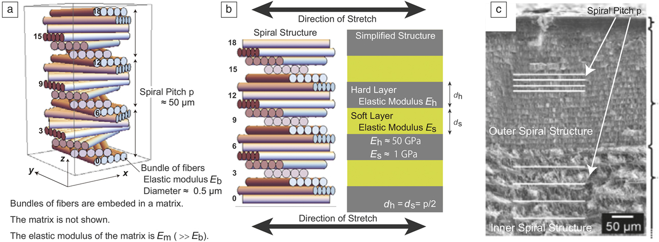
Figure 2. (a) Illustration of the spiral structure of cuticle layers in the exoskeleton of lobsters, generated by Mathematica 10 software. The layers are numbered from 0 to 18. (b) Original spiral structure (left), and its simplified layered structure (right) when the sample is stretched in the specified direction. The layer numbers correspond to those in (a). (c) Scanning electron microscope image of outer and inner spiral structures (exocuticle and endocuticle) with different spiral pitches, observed in the exoskeleton of lobsters. (c) Reproduced with permission from Reference Reference Fabritius, Sachs, Triguero and Raabe41. © 2009 Wiley.
By noting that the fiber bundles are softer than the matrix, the helical structure has been mapped into a layered structure of soft and hard layers of equal thickness, where each layer is a composite of fiber bundles and matrix (as illustrated in Figure 2b).Reference Okumura48 For example, when the sample is stretched in the y direction, as in Figure 2a–b, in the layers numbered 0, 6, 12, and 18, which are a composite of fibers and matrix, fiber direction is parallel to the stretch direction, rendering these layers stronger than the layers numbered 3, 9, and 15, in which the fiber direction is perpendicular to the stretch direction. In other words, the elastic modulus periodically changes along the z-axis when the sample is stretched in the y direction. As a result, on the length scale of the spiral pitch, the structure can be approximately regarded as a layered structure as in the right-hand illustration in Figure 2b.
This structure is similar to the structure of nacre except for (1) the thickness of soft and hard layers are approximately the same (d ≈ d s ≈ d h), and (2) E h and E s are determined to be functions of the elastic moduli of the matrix and bundle, E m and E b, and the volume fractions of the matrix and bundles, φm and φb (for different approaches to the periodically changing elastic modulus, see References Reference Fratzl, Gupta, Fischer and Kolednik33 and Reference Gao49–Reference Kolednik, Predan, Fischer and Fratzl52). The volume fractions can be conveniently parameterized by introducing a small parameter δ where φm = (1 + δ)/2 and φb = (1 − δ)/2, because φm is approximately equal to φb in living lobsters, and the volume fractions satisfy the relation φm + φb = 1.
For this simplified layered structure of the exoskeleton, all four scaling laws, Equations 1, 2, 4, and 6, established for the nacre model, can be exploited if the small parameter ε in these scaling laws is replaced with ε = [(1 + δ)(1 − δ)E m/E b]−1 for the exoskeleton in order to reflect the substructure of fiber bundles and matrix. This is possible because the laws derived for nacre are valid as long as the conditions given in Equation 3 are satisfied. The enhancement factor ε− Reference Meyers, Lin, Seki, Chen, Kad and Bodde1/2(d/a 0) for the fracture energy in Equation 4 can be expressed as:
 $${{\rm{\varepsilon }}^{1/2}}(d/{a_0}) \approx \sqrt {(1 + \delta )(1 - \delta ){E_{\rm{m}}}/{E_{\rm{b}}}} (d/{a_0})\,{\rm{for}}\,{E_{\rm{m}}} &gt; {E_{\rm{b}}}.$$
In addition, when Equation 4 is applied to the exoskeleton, G h is the fracture energy in the toughest direction of a parallel composite in which fiber bundles are oriented parallel to each other throughout the matrix rather than helically. The fracture strength and toughness of this parallel composite is direction-dependent and is strongest when under tension in the direction of the bundles.
The enhancement factor for the fracture energy given in Equation 7 for the exoskeleton is estimated to be a few 1000, which is similar to nacre. This is because in the case of the exoskeleton, the period of the structure d (≈2d s as d s ≈ d h) corresponds to the helical pitch p (≈50 µm) and a 0 to the bundle diameter (≈0.5 µm). Here, rather rough approximations have been utilized for the elastic moduli: The elastic modulus of the matrix (amorphous calcium carbonate) is approximately 50 GPa, and that of the bundles (a composite of chitin fibers and proteins) is around 1 GPa.
By comparing the two enhancement factors in Equations 5 and 7, some differences are noticed in the strategy used for increasing the corresponding enhancement factor for the fracture energy. In nacre, the factor  $\sqrt {{E_{\rm{h}}}/{E_{\rm{s}}}}$, dominates over the other factors, whereas the factor d/a 0 dominates in the exoskeleton. In other words, the combination of extremely soft and hard is exploited in nacre, whereas in the exoskeleton case, the substructures (i.e., the bundles and matrix) are effectively used to adjust helical pitches to enlarge the factor d/a 0 and achieve roughly the same order of fracture toughness. Adjusting the helical pitch has another advantage, which is discussed later.
In the case of the exoskeleton, confirmation of the four scaling laws (for the stress and deformation fields, the maximum stress, and the fracture energy) by experiment or simulation is still under way, however, Equation 4 and Equation 7 support the fact that the following features observed in the exoskeleton are mechanically advantageous. These features can be regarded as guiding principles for toughening, as also supported by theory: (1) The combination of soft and hard elements (i.e., E b < E m); (2) the helical structure, because of which the fracture energy becomes even larger than that in the toughest direction of the parallel structure; (3) the equal volume fractions of the matrix and bundle, which correspond to a sharp peak in the enhancement factor in Equation 7 when δ is zero (i.e., when φm = φb); and (4) the exocuticle with a small helical pitch covers the endocuticle with a large helical pitch, contributing to the reinforcement of the structure in the following manner: A helical structure with a long pitch d cannot be protected against small cracks because Equation 7 is valid for a crack whose size a is larger than d, as suggested in Equation 3. Thus, the exocuticle protects the inside from smaller cracks (but with a lower toughness than the endocuticle), while the endocuticle protects the inside from larger cracks (with a higher toughness than the exocuticle).
Spider webs
Spider silks are high-performance polymeric fibers and thus have been actively studied over the yearsReference Witt and Reed53,Reference Selden54 in terms of their entropic elasticity,Reference Gosline, Denny and DeMont55 water coating,Reference Vollrath and Edmonds56 breaking strength,Reference Osaki57 gene family,Reference Guerette, Ginzinger, Weber and Gosline58 liquid-crystalline structure,Reference Vollrath and Knight59 micellar structure,Reference Jin and Kaplan60,Reference Emile, Le Floch and Vollrath61 hierarchical structure,Reference Zhou and Zhang62 and torsional relaxation.Reference Emile, Le Floch and Vollrath63 The mechanical advantages of spider webs have yet to be explored, except for studies on structural vibration,Reference Masters64,Reference Lin, Edmonds and Vollrath65 tensile pre-stress,Reference Wirth and Barth66 detailed finite-element modeling,Reference Lin, Edmonds and Vollrath65,Reference Alam, Wahab and Jenkins67 and nonlinear response.Reference Cranford, Tarakanova, Pugno and Buehler68–Reference Buehler and Ackbarow70
A simple model of orb spider webs is composed of stiff radial and soft spiral threads and is under a global strain,Reference Aoyanagi and Okumura71 as in real spider websReference Alam, Wahab and Jenkins67 (see Figure 3a–b). It is convenient to introduce a specific spring constant as the spring constant multiplied by the length of the spring (the spring constant is inversely proportional to the length). This quantity can be expressed as the elastic modulus multiplied by the section area of a thread to compare the relative stiffness of the threads. The specific spring constants for the radial and soft threads are denoted K and k, respectively. Typical values of the diameter, elastic modulus, and initial tension of radial threads are 3.9 µm, 1 GPa, and 0.13 mN, respectively, and those of spiral threads are 2.4 µm, 0.8 GPa, and 10 µN, respectively.Reference Alam, Wahab and Jenkins67 These numbers are consistent with other typical values shown in Figure 3c.
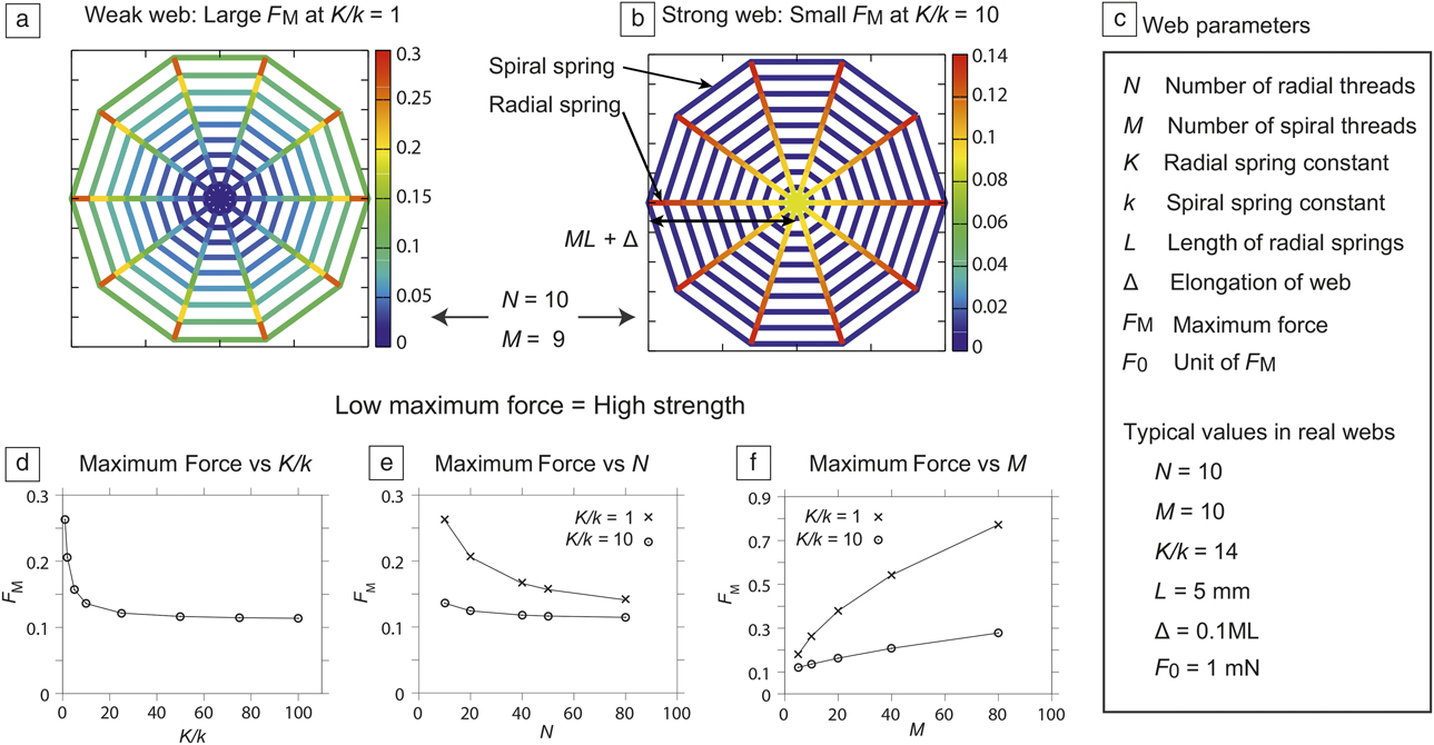
Figure 3. (a–b) Force distribution in a simple model of spider webs under tension. The ratio of radial thread and spiral thread spring constants (multiplied by the length) of (a) and (b) are K/k = 1 and 10, respectively. The maximum force F M that appears at the edge radial thread is smaller in (b), which suggests that real webs (corresponding to [b]) are stronger than artificial webs in which K is comparable to k. (c) Summary of parameters in the model spider web. (d–f) The maximum force F M as a function of K/k, the number of radial threads N, and the number of spiral threads M, respectively. The three plots show that higher K/k values are mechanically advantageous. (a–b) and (d–f) Created from data in Reference Reference Aoyanagi and Okumura71.
As demonstrated in Figure 3a and b, the model web is stronger, that is, a maximum force F M appearing in a web is smaller, when the stiffness contrast K/k is larger than one; as in real webs. Here, the maximum force F M is considered to be a measure of strength, because in general, materials start failing at the position where a strong local force acts.
The simple model of spider webs further reveals surprising conclusions, although the model predicts no scaling laws. The stiffness ratio K/k seems to be optimized in real webs from a number of mechanical viewpoints, giving high adaptability to spiders: (1) In Figure 3d, the maximum force F M sharply drops in a range of small K/k but changes little when K/k is larger than around 14, which is a typical value of the stiffness difference in real webs.Reference Alam, Wahab and Jenkins67 Considering the difficulty for spiders to create two types of thread whose mechanical properties are quite different, the typical value of the stiffness difference of 14 may be regarded as a result of optimization. (2) The weak dependence of the maximum force F M on the number of radial threads N and that of spiral threads M for large K/k (Figure 3e–f, respectively) suggests spiders can be highly flexible to improve their chances of survival. Spiders can spin webs by freely selecting the number of spiral and radial threads, according to the spatial and biological environments, for example, to a typical branch spacing of trees or to a typical size of prey. (3) This model also explains how spider webs function well even if some parts of spiral threads are missing. Remarkably, stress concentration is absent in spider webs.
Conclusion
A key feature in the reinforcement on the three biological materials discussed here, nacre, the crustacean’s exoskeleton, and spider webs, is the combination of soft and hard elements. Simple models reveal that the structures are optimized in a number of mechanical senses, and simple scaling laws or simple physical understandings provide guiding principles for developing tough materials mimicking the biological structures. It is possible that such a naive model is oversimplified and fails to capture the reality of the original material. Even in such a case, simple guiding principles obtained from a biologically inspired study are useful in their own right and could lead to the development of an artificial material that is even stronger than the original biological material. This fact further justifies the importance of studies on complex systems via simple models.
An extreme example of soft-hard composites is porous materials with voids corresponding to the soft element. In fact, there are many porous and strong materials in nature, such as the stereom of holothurians (e.g., the soft bone of sea cucumbers),Reference Emlet72 the skeleton of a certain sponge,Reference Aizenberg, Weaver, Thanawala, Sundar, Morse and Fratzl73 and the frustules (hard cell walls) of diatoms.Reference Hamm, Merkel, Springer, Jurkojc, Maier, Prechtel and Smetacek74 Accordingly, studies on reinforcement with voids would be an interesting direction of research.Reference Shiina, Hamamoto and Okumura75,Reference Kashima and Okumura76 Nonlinear extension of the simple models would also play an important role in the future study of biological materials and biomaterials.Reference Nakagawa and Okumura39,Reference Aoyanagi and Okumura40,Reference Soné, Mori and Okumura77
Approaches via a simple model, often using scaling laws, are promising and have been accepted, especially in fields in which engineering or material scientists meet physicists, for example, in polymer science,Reference Kashima and Okumura76,Reference de Gennes78 wetting,Reference de Gennes, Brochard-Wyart and Quéré79,Reference Yokota and Okumura80 and granular physics.Reference de Gennes81,Reference Takehara and Okumura82 This review will be useful for disseminating the perspective of physicists for complex systems in fields in which such simple approaches have yet to be used, including fields concerning fracture and toughness of materials.
Acknowledgments
This research was supported by Grant-in-Aid for Scientific Research on Innovative Areas, “Fusion Materials (Area no. 2206),” of MEXT, Japan, by a Grant-in-Aid for Scientific Research (A) (No. 24244066) of JSPS, Japan, and by the ImPACT Program of the Council for Science, Technology and Innovation (Cabinet Office, Government of Japan).


 Open access