


1. Introduction
As a result of commercial availability of highly dense single nucleotide polymorphism (SNP) chips in humans, genome-wide association analysis (GWAS) has proven to be a powerful tool to identify genes for common diseases and complex traits (Hirschhorn & Daly, Reference Hirschhorn and Daly2005; Visscher et al., Reference Visscher, Macgregor, Benyamin, Zhu, Gordon, Medland, Hill, Hottenga, Willemsen, Boomsma, Liu, Deng, Montgomery and Martin2007). Similarly, GWAS has been applied to animals for the discovery of genes that are associated with disease and production traits (Karlsson et al., Reference Karlsson, Baranowska, Wade, Salmon Hillbertz, Zody, Anderson, Biagi, Patterson, Pielberg, Kulbokas, Comstock, Keller, Mesirov, von Euler, Kampe, Hedhammar, Lander, Andersson, Andersson and Lindblad-Toh2007; Bennett et al., Reference Bennett, Farber, Orozco, Kang, Ghazalpour, Siemers, Neubauer, Neuhaus, Yordanova, Guan, Truong, Yang, He, Kayne, Gargalovic, Kirchgessner, Pan, Castellani, Kostem, Furlotte, Drake, Eskin and Lusis2010; Bolormaa et al., Reference Bolormaa, Pryce, Hayes and Goddard2010; Orr et al., Reference Orr, Back, Gu, Leegwater, Govindarajan, Conroy, Ducro, Van Arendonk, MacHugh, Ennis, Hill and Brama2010; Pryce et al., Reference Pryce, Bolormaa, Chamberlain, Bowman, Savin, Goddard and Hayes2010). In animal breeding, a closely related procedure that makes use of the same SNP chips, but for an entirely different purpose, is the genomic estimation of breeding values (GEBVs) for genomic selection (GWMAS), a form of marker-assisted selection. GWMAS is often performed with procedures called BayesA or BayesB that consider all genetic associations derived from markers (Meuwissen et al., Reference Meuwissen, Hayes and Goddard2001). Moreover, BayesA and BayesB solutions provide SNP effects; thus, these methods can be applied to GWAS (Goddard & Hayes, Reference Goddard and Hayes2009; Sun et al., Reference Sun, Fernando, Garrick and Dekkers2011) with the additional advantage of accounting for population stratification and cryptic relatedness (Sillanpaa, Reference Sillanpaa2011). The classical GWAS (CGWAS) is based on a test of a single marker, which treats each SNP marker as a covariate in the model (Hirschhorn & Daly, Reference Hirschhorn and Daly2005). The main advantage of CGWAS is the ease of significance testing; however, it is likely to result in reduced fit to the data compared with methods where all SNPs are jointly considered. Additionally, neither Bayesian methods nor single-marker analysis can directly include genetic association found in the pedigree of animals that have not been genotyped. Although such information can be considered indirectly in multiple-step procedures in which phenotypic data from relatives are summarized to create pseudo-data for genotyped individuals (VanRaden et al., Reference VanRaden, Van Tassell, Wiggans, Sonstegard, Schnabel, Taylor and Schenkel2009), new problems can arise, such as information loss, heterogeneity caused by different amounts of information in the original dataset and bias (Vitezica et al., Reference Vitezica, Aguilar, Misztal and Legarra2011). Thus, multiple-step methods for computing genomic predictions are not only complicated but likely suboptimal for GWAS. This is particularly true in livestock species, where pedigrees are complex, and nuclear families are the exception rather than the rule. In contrast Misztal et al. (Reference Misztal, Legarra and Aguilar2009) and Christensen & Lund (Reference Christensen and Lund2010) proposed a single-step GBLUP (ssGBLUP) that integrates phenotypes, genotypes and pedigree information. Such information can be combined with genomic data for greater detection power and estimation precision through a properly scaled and augmented relationship matrix (Legarra et al., Reference Legarra, Aguilar and Misztal2009; Misztal et al., Reference Misztal, Legarra and Aguilar2009). The ssGBLUP method has been shown to provide more consistent solutions and better accuracy than the multiple-step approach (Aguilar et al., Reference Aguilar, Misztal, Johnson, Legarra, Tsuruta and Lawlor2010; Chen et al., Reference Chen, Misztal, Aguilar, Legarra and Muir2011; Forni et al., Reference Forni, Aguilar and Misztal2011).
A limitation of the ssGBLUP methodology is that it is based on an infinitesimal model, which assumes equal variance for all SNP marker-QTL associated effects. An advantage of the infinitesimal model is that the resulting genomic relationship matrix is identical for all traits within a population (Aguilar et al., Reference Aguilar, Misztal, Johnson, Legarra, Tsuruta and Lawlor2010). In contrast, although BayesA or BayesB is limited in that neither can include phenotypic information from non-genotyped individuals, they remove the assumption of equal variance for all SNP marker-QTL associated effects, which appears to be a more realistic situation. Unfortunately, relaxing this assumption comes at a cost of orders of magnitude more computing time in a Bayesian framework. Combining the strengths of both methods (i.e. allowing for unequal variances in an ssGBLUP context) could improve the accuracy of the estimation of GEBVs for breeding and selection applications, and precision for the estimation of SNP effects for GWAS applications.
Estimation of weights for SNP variances can be achieved without sampling. Zhang et al. (Reference Zhang, Liu, Ding, Bijma, de Koning and Zhang2010) derived SNP weights as functions of squares of SNP effects and incorporated those variances as weights in GBLUP. Sun et al. (Reference Sun, Fernando, Garrick and Dekkers2011) developed an iterative procedure for GBLUP, in which GEBVs were converted to SNP effects and weights were obtained similar to those in Zhang et al. (Reference Zhang, Liu, Ding, Bijma, de Koning and Zhang2010) . However, neither study could directly utilize phenotypes of ungenotyped animals.
The objectives of this research were to investigate the optimal weights on marker variances for improving accuracy and precision in GWAS and GEBVs by ssGBLUP, and to compare results from ssGBLUP, CGWAS and the BayesB methods as described by Meuwissen et al. (Reference Meuwissen, Hayes and Goddard2001) .
2. Materials and methods
(i) Data simulation
Data were simulated using QMSim (Sargolzaei & Schenkel, Reference Sargolzaei and Schenkel2009) for an additive trait with a mean of 5·0, phenotypic variance 1·0 and heritability 0·5. Two 100 cM chromosomes were simulated, with each chromosome containing 15 uniformly distributed QTLs. For chromosome 1 and chromosome 2, on average 1552 and 1448 SNP markers, respectively, were evenly distributed. Both SNP markers and QTLs were assumed to be bi-allelic, and no marker loci overlapped with the QTLs. Minor allele frequencies were >0·05. Effects of QTLs were randomly sampled from a Gamma distribution with a shape factor of 0·4 and a scale factor of 1·36. All additive genetic variance resulted from the QTLs. A simulated population started at generation 1001 (i.e. base population) and consisted of 100 individuals. For generations, 1001 to 1, mutation rate of 0·000025 was simulated for each locus of both QTLs and SNPs per generation, and non-overlapping generations were simulated with population size per generation increasing gradually from 100 to 2800. In generations 0–4, 80 randomly chosen males and 520 randomly chosen females were genotyped and produced 2600 progenies by random mating. The phenotypic information was recorded for all animals in generations 0–5. Genotypes were recorded for all parents in generations 3 and 4, and 300 random individuals in generation 5. For recent generations 0–5, the complete datasets contained 15 800 individuals in pedigree with records, of which 1500 individuals were genotyped. The simulation was replicated ten times. Some statistics of the simulated dataset are shown in Table 1.
Table 1. Description of genomic data from simulation
* SDs: standard deviations.
† Chr1 and Chr2: chromosome 1 and chromosome 2.
‡ Average minor allele frequencies of SNPs.
§ Average effects of QTLs.
(ii) Model and methodology
The single-trait model for ssGBLUP was
where y is a vector of simulated observations (phenotypes), 1 is a vector of all ones, μ is the overall mean of phenotypic records, Za is an incidence matrix that relates individuals to phenotypes, a is a vector of individual animal effects and e is a vector of residuals. The variances of a and e are
where σ a 2 and σ e 2 are total genetic additive and residual variances, respectively, and H is a matrix that combines pedigree and genomic relationships as in Aguilar et al. (Reference Aguilar, Misztal, Johnson, Legarra, Tsuruta and Lawlor2010), and its inverse is
where A is a numerator (pedigree) relationship matrix for all animals; A22 is a numerator relationship matrix for genotyped animals; and G is a genomic relationship matrix. Matrix G was constructed based on VanRaden et al. (Reference VanRaden, Van Tassell, Wiggans, Sonstegard, Schnabel, Taylor and Schenkel2009) that assumed allele frequencies of the current population and adjusted for compatibility with A22 , which was applied in ‘GC’ and ‘BLUPα’ in Chen et al. (Reference Chen, Misztal, Aguilar, Legarra and Muir2011) and Vitezica et al. (Reference Vitezica, Aguilar, Misztal and Legarra2011) .
(iii) Derivation of SNP effects from breeding values
Let the animal effects be decomposed into those for genotyped (ag ) and ungenotyped (an ) animals. The animal effects of genotyped animals are a function of SNP effects:
whereZ is a matrix relating genotypes of each locus andu is a vector of SNP marker effects.
Thus, the variance of the animal effects is
where D is a diagonal matrix of weights for variances of SNPs (D=I for GBLUP), σ u 2 is the genetic additive variance captured by each SNP marker when no weights are present and G* is the weighted genomic relationship matrix.
The joint (co)variance of animal effects (ag ) and SNP effects (u) is
subsequently
where λ is a variance ratio or a normalizing constant. According to VanRaden et al. (Reference VanRaden, Van Tassell, Wiggans, Sonstegard, Schnabel, Taylor and Schenkel2009),

where M is the number of SNPs and pi is the allele frequency of the second allele of the ith marker. Following Stranden & Garrick (Reference Stranden and Garrick2009) one can derive
Therefore, the equation for predicting SNP effects which uses weighted genomic relationship matrix G* becomes
This is the best predictor of SNP effects given animal effects (Henderson, Reference Henderson1973). Estimates of SNP effects can be used to estimate individual variance of each SNP effect (Zhang et al., Reference Zhang, Liu, Ding, Bijma, de Koning and Zhang2010):
(iv) Computing algorithm
The above formulae can be used to create an algorithm for estimation of D from ssGBLUP. Denote t as an iteration number and i as the ith SNP. The algorithm proceeds as follows:
1. t=0, D(t)=I;G*(t)=ZD(t) Z ′ λ.
2. Compute
 by ssGBLUP.
3. Calculate
4. Calculate
for all i as in Zhang et al. (Reference Zhang, Liu, Ding, Bijma, de Koning and Zhang2010)
.5. Normalize
6. Calculate
7. t=t+1.
8. Exit, or loop to step 2 or 3.
In looping to step 3 (scenario S1), one applies the revised G* only for the prediction of SNP effects, while calculating the animal effects only once, thus ![]() does not change during iterations. In looping to step 2 (scenario S2), both animal and SNP effects are recomputed. Whether scenario S1 is sufficient as opposed to scenario S2 and how much iterations are necessary is not clear and needs to be determined experimentally. In particular, scenario S1 is applicable to multiple-trait models where the relationship matrix needs to be identical for all traits.
does not change during iterations. In looping to step 2 (scenario S2), both animal and SNP effects are recomputed. Whether scenario S1 is sufficient as opposed to scenario S2 and how much iterations are necessary is not clear and needs to be determined experimentally. In particular, scenario S1 is applicable to multiple-trait models where the relationship matrix needs to be identical for all traits.
(v) Computations
Computations with ssGBLUP involved program BLUPF90 (Misztal et al., Reference Misztal, Tsuruta, Strabel, Auvray, Druet and Lee2002) modified for genomic analyses (Aguilar et al., Reference Aguilar, Misztal, Johnson, Legarra, Tsuruta and Lawlor2010), and used simulated parameters. Comparisons involved BayesB procedure as implemented in the GenSel package (Habier et al., Reference Habier, Fernando, Kizilkaya and Garrick2010). These procedures used the model:
where ![]() is a dependent variable (DV) for genotyped animals, with options being non-weighted deregressed proofs (DP) or weighted DP (Stranden & Garrick, Reference Stranden and Garrick2009). For non-weighted DP, all weights were assumed equal to each other being 1; for weighted DP, the weight for ith individual was calculated as
is a dependent variable (DV) for genotyped animals, with options being non-weighted deregressed proofs (DP) or weighted DP (Stranden & Garrick, Reference Stranden and Garrick2009). For non-weighted DP, all weights were assumed equal to each other being 1; for weighted DP, the weight for ith individual was calculated as
based on equation (10) in Garrick et al. (Reference Garrick, Taylor and Fernando2009), where c is the fraction of the genetic variance not accounted for by SNPs, and was assumed to be 0·1 (Ostersen et al., Reference Ostersen, Christensen, Henryon, Nielsen, Su and Madsen2011), h 2 is the heritability and ri
2 is reliability of DP for the ith individual. Moreover, 1 is a vector of all ones, μ is the overall mean, Zu
is a matrix relating SNP marker effects to phenotypic information, u is a vector of SNP marker effects, e is a vector of residuals distributed as N(0, Db
σ
e
2), where Db
is a vector of weights as in Stranden & Garrick (Reference Stranden and Garrick2009)
. For BayesB, marker effects were assumed to be distributed as ![]() , where
, where ![]() is the variance of the jth SNP, and the proportion of SNPs with no effects (
is the variance of the jth SNP, and the proportion of SNPs with no effects (![]() ) was set to 90%. As for ssGBLUP, the total genetic variance of BayesB methods was equal to the simulated value of 0·5. Priors for variances of SNP effects and residuals followed a scaled inverse Chi-square distribution with degrees of freedom 4 and 10, respectively. The Monte Carlo Markov Chain was run for 100 000 iterations (first 10 000 rounds were discarded as burn-in) with Gibbs sampling, with 100 of Metropolis–Hastings sampling within each Gibbs sampling cycle. Estimates of GEBVs and SNP effects were based on the posterior means according to the remaining 90 000 iterations. Accuracies of genotyped animals were defined as correlations between true breeding values (TBVs) and GEBVs. Accuracy of GWAS was determined by correlations of QTL effects with the sum of m SNP solutions adjacent to each QTL, where m varied from 1 to 40. We did not attempt to declare detection thresholds, or P-values, because they are difficult to define and compare with classical frequentist test of hypothesis, in the context of shrunken or Bayesian estimators, as is the case here (Servin & Stephens, Reference Servin and Stephens2007; Wakefield, Reference Wakefield2009).
) was set to 90%. As for ssGBLUP, the total genetic variance of BayesB methods was equal to the simulated value of 0·5. Priors for variances of SNP effects and residuals followed a scaled inverse Chi-square distribution with degrees of freedom 4 and 10, respectively. The Monte Carlo Markov Chain was run for 100 000 iterations (first 10 000 rounds were discarded as burn-in) with Gibbs sampling, with 100 of Metropolis–Hastings sampling within each Gibbs sampling cycle. Estimates of GEBVs and SNP effects were based on the posterior means according to the remaining 90 000 iterations. Accuracies of genotyped animals were defined as correlations between true breeding values (TBVs) and GEBVs. Accuracy of GWAS was determined by correlations of QTL effects with the sum of m SNP solutions adjacent to each QTL, where m varied from 1 to 40. We did not attempt to declare detection thresholds, or P-values, because they are difficult to define and compare with classical frequentist test of hypothesis, in the context of shrunken or Bayesian estimators, as is the case here (Servin & Stephens, Reference Servin and Stephens2007; Wakefield, Reference Wakefield2009).
For comparisons, SNP solutions were also estimated by CGWAS using a ‘Snappy’ approach implemented in WOMBAT (Meyer & Tier, Reference Meyer and Tier2012). When CGWAS analyses are repeated for a large number of SNPs, the computing time can be large, especially for large SNP panels. In ‘Snappy’, matrices common to all SNPs are pre-computed, greatly reducing the computation time for the complete scan.
3. Results and discussion
(i) Accuracy of estimated breeding values (EBVs)
EBVs had been obtained through regular BLUP, ssGBLUP and Bayesian methods (BayesB using non-weighted or weighted DP), respectively. Accuracies of genotyped animals are shown in Table 2, and defined as correlations between TBVs and EBVs: EBVs for regular BLUP and GEBVs for other approaches. Accuracies of ssGBLUP ranged from 0·87 (0·02) to 0·89 (0·01) depending on iterations, and they were always higher than EBVs for BLUP. For S1, accuracies of GEBVs remained 0·87 (0·01). This result occurred because GEBVs were not recomputed (only SNP effects). For S2, however, the accuracy increased to 0·89 (0·01) by the second round, then dropped to 0·88 (0·01 or 0·02) until the sixth round, and then dropped to 0·87 (0·02). The slight decrease of accuracy in the later rounds could be due to excessive weights given to SNPs associated with few QTLs with larger effects, and reduced weights for numerous QTLs with smaller effects.
Table 2. Correlations (SDs) between TBVs from simulation with EBVs and DP from regular BLUP, GEBVs from ssGBLUP and from BayesB with non-weighted and weighted (c=0·1) DP
* GEBV solutions using ssGBLUP from iteration 1 (it1) to iteration 8 (it8).
† Non-weighted DP, and weighted DP with c=0·1.
For BayesB methods, the accuracies of non-weighted DP were 0·88 (0·02) and were the same as the result of weighted DP (c=0·1). As using DP as DV yields more reliable breeding value solutions than using EBVs in genetic evaluation (Ostersen et al., Reference Ostersen, Christensen, Henryon, Nielsen, Su and Madsen2011), other types of DV (e.g. phenotypic records and EBVs) were not considered in this study. For both scenarios of using non-weighted and weighted DP as DV, accuracies from BayesB methods were similar to ssGBLUP with slightly larger standard deviations (SDs) across replications. Although the Bayesian methods lose accuracies when pseudo-data are used (Vitezica et al., Reference Vitezica, Aguilar, Misztal and Legarra2011) that loss of accuracy seems to be similar to the loss of accuracy in ssGBLUP by assuming variances of all SNPs are equal. In the work of Vitezica et al. (Reference Vitezica, Aguilar, Misztal and Legarra2011), genotyped animals do not have observations of their own, whereas here genotyped animals do have associated phenotypes. Therefore information from related animals added little to EBV accuracies.
(ii) Accuracy of QTL estimates
Table 3 presents accuracies of ssGBLUP for QTLs defined as correlations between QTL effects and the sum of m adjacent SNP marker effects, where m varied from 1 to 40. SNP effects under scenarios of S1 and S2 were updated iteratively resulting in similar results. For both S1 and S2, and all iterations, accuracies of QTLs increased from m=1 to m=8, and decreased sharply for m=40. Iterations improved the accuracy of the S1 and S2 options but only for m=8 and m=16. With iteration and subsequent recomputation of SNP weights, small SNP effects were reduced every round while the large effects became even larger. Iteration for new GEBVs (S2) allowed corrections to SNP with small effects. The highest correlation at m=1, 2 and 4 was after the first iteration. The highest correlation was 0·82 with m=8 and the second iteration. In both S1 and S2, iteration for GEBVs maximized the accuracy of GEBVs given weights. The highest accuracy was achieved by having a combination of weights that minimized estimation errors but reflected the reality that SNPs adjacent to a QTL contribute to estimation of that QTL.
Table 3. Average correlations (SDs) between QTL effects and sum of cluster of m SNP effects using ssGBLUP
* S1: update weights for SNP effects but not for GEBVs; S2: update weights for both GEBVs and SNP effects in each iteration.
† Number of SNPs (i.e. m ranges from 1 to 40) in each cluster.
The advantage of S2 over S1 is dependent on the number and distribution of QTL effects. With many QTL effects and relatively equal distribution, assigning differential weights to SNPs does not greatly improve the accuracy of GEBVs, and therefore little is gained by iteration on GEBVs. Greater improvements with S2 are expected when differential weights on SNP improve accuracy to a greater degree. In a separate study (results not reported), the realized accuracy of S2 improved up to the third iteration for some traits, while deteriorating for other traits in subsequent round. Further research may establish an optimum number of rounds for each particular situation.
Relatively lower correlations are not unexpected at low m. Zondervan & Cardon (Reference Zondervan and Cardon2004)
have found that the closest SNP marker is not always the best predictor of its neighbouring QTL. There should be an ‘optimal haplotype length’ according to the marker density and extent of linkage disequilibrium in the population (Villumsen et al., Reference Villumsen, Janss and Lund2009). Density of SNP markers and QTLs in the simulated genome was, on average, 0·067 and 6·06 cM, respectively. With each QTL distributed approximately every 90 SNP markers, the QTL effects could be best approximated by the sum of the adjacent 90 SNP effects. However, due to recombination and mutation for 1000 generations, the best haplotype length can be much shorter than expected. In this study, approximations with eight SNPs were the most accurate, while those with close to 40 or more were not. Decreases of accuracies in later iterations can be explained by excessive weights on larger SNPs in later iterations. A different algorithm to calculate weights of SNP effects, e.g. with a lower bound similar to Sun et al. (Reference Sun, Fernando, Garrick and Dekkers2011), may improve accuracies in later rounds. The form of constructing weights used here is indeed suboptimal, because it considers that the estimate of the jth SNP effect ![]() is the true value, whereas in fact it is a regressed value. An optimal procedure would consider the uncertainty in the estimation of SNP effects by expectation–maximization (EM) or by Bayesian procedures (Xu, Reference Xu2010; Legarra et al., Reference Legarra, Robert-Granie, Croiseau, Guillaume and Fritz2011).
is the true value, whereas in fact it is a regressed value. An optimal procedure would consider the uncertainty in the estimation of SNP effects by expectation–maximization (EM) or by Bayesian procedures (Xu, Reference Xu2010; Legarra et al., Reference Legarra, Robert-Granie, Croiseau, Guillaume and Fritz2011).
Table 4 shows the correlation between QTL effects and the sum of m adjacent SNP solutions for BayesB using non-weighted or weighted DP and for CGWAS using non-weighted DP. When BayesB was applied, weighting DP had little effect on the correlations, which most likely was due to the simple population structure in our simulated study and subsequently similar weights for most genotyped animals. Compared with ssGBLUP and iteration 1, the correlations resulting from application of BayesB were smaller for m⩽4 and slightly higher for m⩾16. Although the average correlations using BayesB were the same as, or even slightly better than when ssGBLUP was used, the SDs calculated over 10 replications were much higher for BayesB than ssGBLUP. Even in the best situation, the SDs were 0·07 for BayesB with m=16, as compared to 0·02 (or 0·03) for ssGBLUP/S1 (or S2) with m=8. For other m, SDs ranged from 0·08 to 0·27 for BayesB, and from 0·02 to 0·09 for ssGBLUP. Larger SDs with BayesB could be due to its sampling structure (Gianola et al., Reference Gianola, de los Campos, Hill, Manfredi and Fernando2009), which also made BayesB less robust than ssGBLUP. With CGWAS, the correlations were higher than any other methods with m=1, matched ssGBLUP in iteration 1 with m=2, and were lower than the other methods with m⩾4. Due to fitting a single SNP as a fixed effect, CGWAS is best for identifying a single causative SNP, but seems less efficient in identifying regions containing the QTLs. In general, SDs with CGWAS were lower than with BayesB, but higher than with ssGBLUP.
Table 4. Average correlations (SDs) between QTL effects and sum of cluster of m SNP effects using BayesB and WOMBAT

* DP used as DV in BayesB and classical GWAS using WOMBAT.
† Non-weighted DP and weighted DP with c=0·1.
‡ Number of SNPs (i.e. m ranges from 1 to 40) in each cluster.
(iii) Graphs of SNP solutions and their moving averages
Figures 1–4 present SNP solutions or their four-point moving averages for several methods. The graphs of SNP solutions are the least noisy for BayesB, and the noisiest for CGWAS, with ssGBLUP in between. While most SNP solutions in BayesB are set to 0, lack of shrinkage in CGWAS results in solutions with more noise. Solutions from the third iteration of ssGBLUP/S1 were more similar to those of BayesB, as each round of ssGBLUP shrinks smaller solutions. With averaging, graphs from all the methods were more similar, with closest similarity between BayesB and ssGBLUP/S1 in iteration 3, and CGWAS and ssGBLUP in iteration 1. The similarities confirm that for this particular dataset, most QTLs cannot be located with a single SNP accurately; however, all of the methods are similar in identifying regions containing large QTLs.
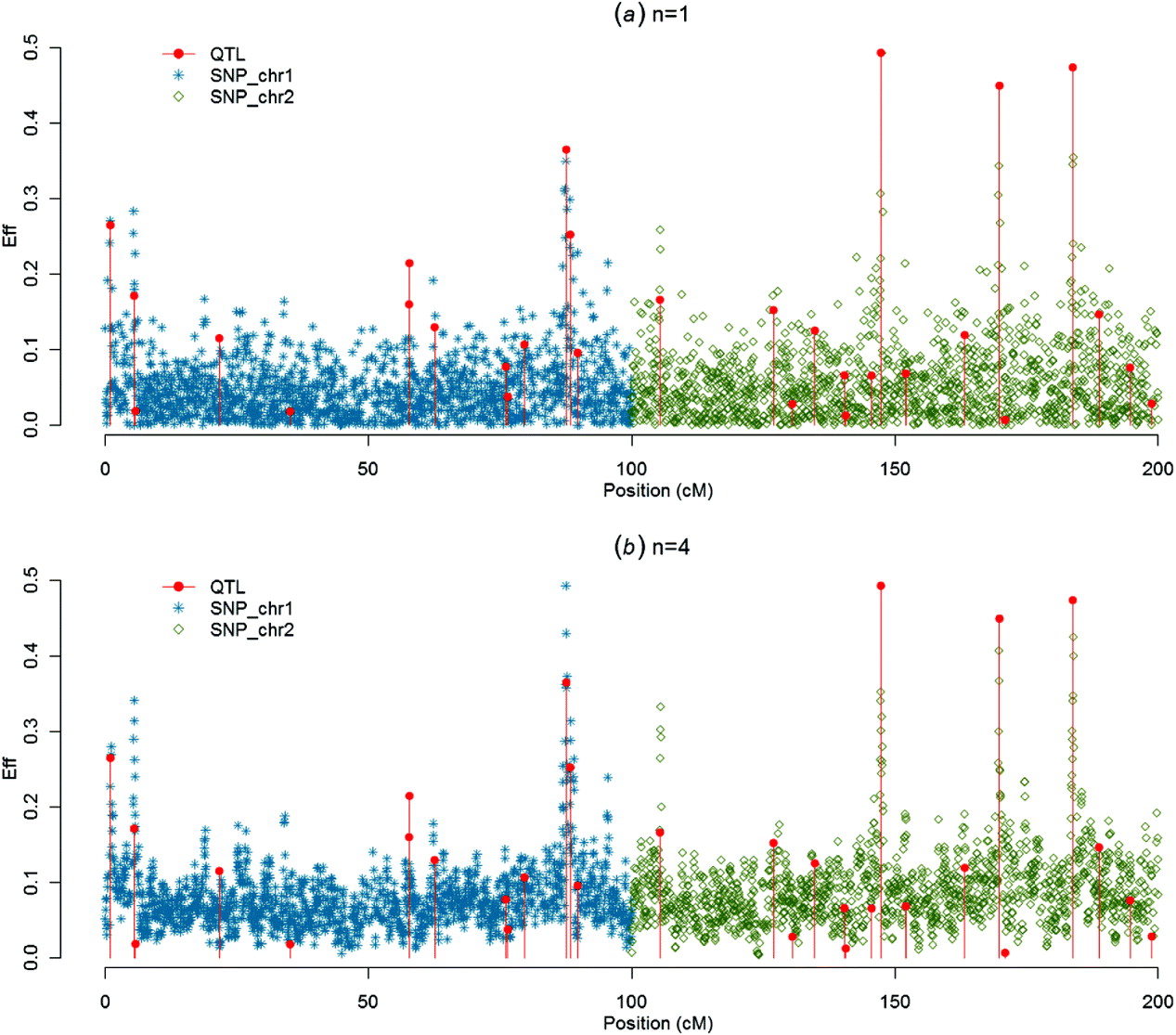
Fig. 1. SNP solutions and their four-point moving averages from ssGBLUP/S1 and ssGBLUP/S2 in the first iteration: (a) SNP solutions and (b) four-point moving average.
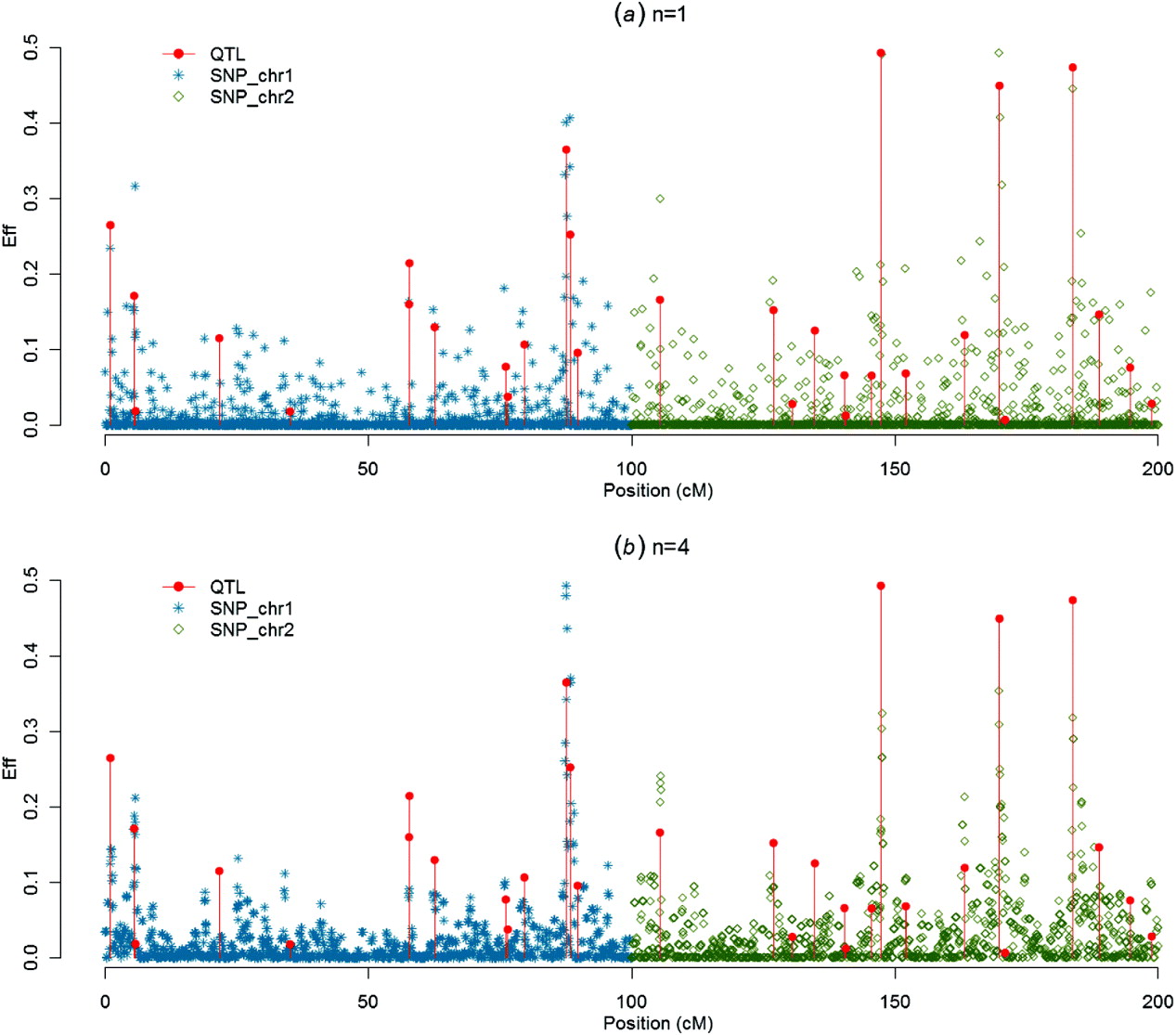
Fig. 2. SNP solutions and their four-point moving averages from ssGBLUP/S1 in the third iteration: (a) SNP solutions and (b) four-point moving average.
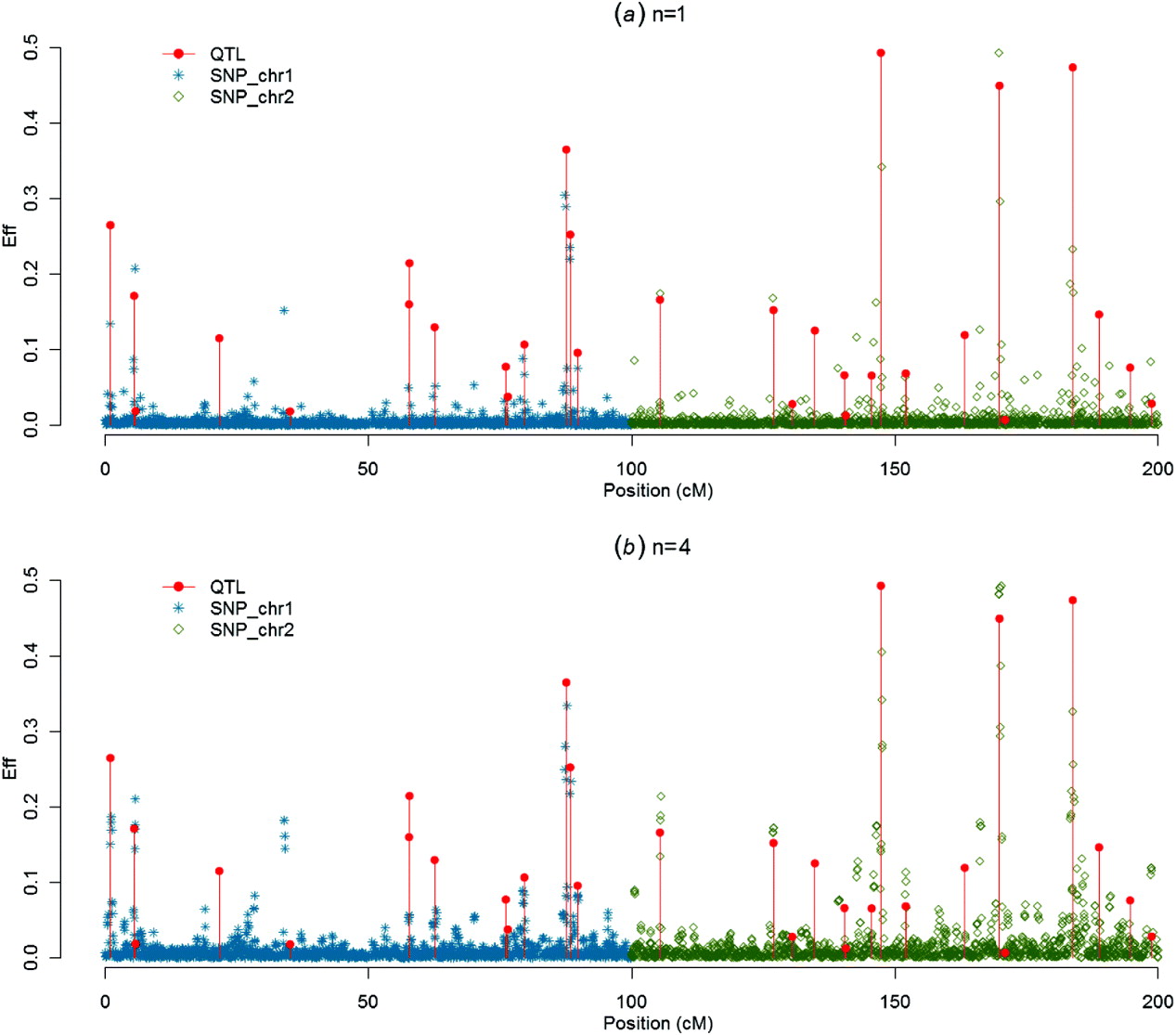
Fig. 3. SNP solutions and their four-point moving averages from BayesB with weighted DP (c=0·1) as the DV: (a) SNP solutions and (b) four-point moving average.
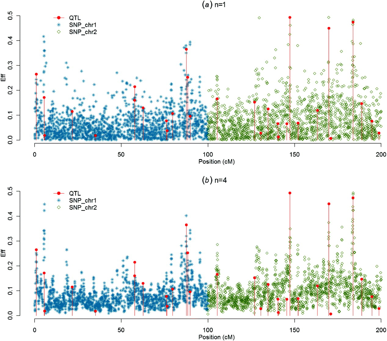
Fig. 4. SNP solutions and their four-point moving averages from r with non-weighted DP as the DV: (a) SNP solutions and (b) four-point moving average.
(iv) Computing considerations
In terms of computing time, one round of ssGBLUP required about 2 min, a run of BayesB required about 5 h, and a run of WOMBAT only required 13 s. Long running time in BayesB is due to long sampling. The extraordinarily fast run in WOMBAT is due to an ingenious algorithm; in testing, WOMBAT was over 100 times faster than previous CGWAS approaches. However, the timing analyses were not fully comparable. Both BayesB and ssGBLUP are useful for creating prediction equations based on computed SNP effects, while CGWAS is only useful for GWAS. Comparisons based on computing times are not complete, as BayesB and CGWAS require a BLUP run to create DP, but no such step is required with ssGBLUP.
When implemented efficiently, the cost of BayesB is linear for the number of SNPs and the number of subjects (Legarra & Misztal, Reference Legarra and Misztal2008). As currently implemented, the creation of G −1 in ssGBLUP is linear with respect to the number of SNPs and cubic with respect to the number of subjects (Aguilar et al., Reference Aguilar, Misztal, Legarra and Tsuruta2011). With efficient implementation, the time to create G −1 is about 1 min for 7k genotypes and 1 h for 30k genotypes (Aguilar et al., Reference Aguilar, Misztal, Legarra and Tsuruta2011). The ssGBLUP method has a potential of smaller than cubic cost with respect to the number of genotypes with non-symmetric mixed model equations and preconditioned conjugate gradients (PCG) iteration (Misztal et al., Reference Misztal, Legarra and Aguilar2009; Legarra & Ducrocq, Reference Legarra and Ducrocqsubmitted).
(v) Additional considerations
In practice, GWAS (as practiced in humans) seeks to find loci strongly associated across ‘unrelated’ individuals. Genomic selection works with closely related populations, and this relation generates strong linkage (disequilibrium) within the sample that cannot be ignored. As results from the three methods are similar, none of the methods do a particularly good job of distinguishing associations from that due to linkage disequilibrium. Additional analyses are required to determine whether markers with large effects are due to associated loci or to linkage disequilibrium.
For the datasets in this study, in the best case, ssGBLUP delivered more accurate GEBVs than the best-case BayesB. All the methods delivered similar predictions of QTL effects based on the sum of 2-SNP effects. The ssGBLUP/S1 method is still relatively new and can benefit from further refinements. In particular, the refinements would involve more accurate sampling of SNP variances as discussed before, and a determination of the optimum number of rounds in ssGBLUP/S2 for maximum accuracy of GEBVs and GWAS. Another needed refinement for ssGBLUP is methodology for significance testing. Without such testing, the use of ssGBLUP for GWAS is limited to identifying SNPs or regions of SNPs with very large effects.
In general, ssGBLUP/S1 seems to provide more consistent estimates than either BayesB or CGWAS using DP. The ssGBLUP/S1 method is also much simpler and therefore more robust to run as: (i) no pseudo-data are required and (ii) no sampling is used. Mrode et al. (Reference Mrode, Coffey, Stradén, Meuwissen, Kaam, Kearney and Berr2010) found large differences regarding results and computing time among various implementations of BayesB.
Models used in this study were very simple with a relatively balanced population structure. For complicated models, such as a multi-trait, maternal effect, random regression or reaction norm models, DP are hard or near impossible to create. Even if they can be created, approximations of DP (Vitezica et al., Reference Vitezica, Aguilar, Misztal and Legarra2011) would reduce accuracy. The performance of ssGBLUP is likely to improve with field data and more complex models with additional refinements.
4. Conclusions
The ssGBLUP method can be modified to compute SNP effects and estimate variances of SNP effects. Such modifications allow for increased accuracy of GEBVs and enable GWAS. The main advantage of ssGBLUP for GWAS is the ability to incorporate phenotypes of ungenotyped animals directly in a BLUP-like approach, without computing pseudo-data. Modified ssGBLUP may become the method of choice for GWAS in the case where merely a fraction of the population with phenotypes is genotyped. In which case, the model for analysis is too complex for use of other methods, and pseudo-data, such as DP, for use with method BayesB and CGWAS, cannot be obtained with sufficient accuracy. In addition, ssGBLUP has the advantages of fast computing, robust estimates and simplicity.
We acknowledge helpful discussions and pointing to the Zhang et al. (Reference Zhang, Liu, Ding, Bijma, de Koning and Zhang2010) study by R. L. Fernando. We used moving averages of SNP solutions following examples by J. Dekkers. This study was partially funded by the Holstein Association and Agriculture and Food Research Initiative grants 2009-65205-05665 and 2010-65205-20366 from the USDA National Institute of Food and Agriculture Animal Genome Program.


 Open access