


I. INTRODUCTION
The video-plus-depth representation for multiview video sequences (MVDs) consists of several views of the same scene with their associated depth information, which is the distance from the camera for every point in the view. The MVD representation allows functionalities like three-dimensional (3D) television and free-viewpoint video [Reference Marpe, Wiegand and Sullivan1–Reference Guillemot, Pereira, Torres, Ebrahimi, Leonardi and Ostermann3], but it generates large volumes of data that need to be compressed for storage and transmission. As a consequence, MVD compression has attracted a huge amount of research effort in the last years, while ISO and ITU are jointly developing an MVD coding standard [4]. Compression should exploit all kinds of statistical dependencies present in this format: spatial, temporal, and inter-view, but also inter-component dependencies, i.e. between color (or texture) and depth data [Reference Merkle, Smolic, Müller and Wiegand5, Reference Dufaux, Pesquet-Popescu and Cagnazzo6].
We focus in particular on depth images compression through contour-based coding means. The techniques developed for texture images are not well suited for depth images, since the latter have different properties and they are not meant to be visualized but only used for rendering of virtual views. Objects within a depth map are usually arranged along planes in different perspectives; as a consequence, there are areas of smoothly varying levels, separated by sharp edges corresponding to object boundaries. These characteristics call for an accurate encoding of contour information. Some of the proposed approaches include modeling the depth signal as a piecewise polynomials (wedgelets and platelets [Reference Merkle, Morvan, Smolic, Farin, Mueller and Wiegand7]), where the smooth parts are separated by the object contours. However, it is generally recognized that a high-quality view rendering at the receiver side is possible only by preserving the contour information [Reference Gautier, Le Meur and Guillemot8, Reference Shen, Kim, Narang, Ortega, Lee and Wey9], since distortions on edges during the encoding step would cause a sensible degradation on the synthesized view and on the 3D perception. In other words, a lossless or quasi lossless coding of the contour is practically mandatory.
For these reasons, in this paper we focus on lossless coding of contours, and we target as natural application the compression of depth maps. However, we observe that an effective contour coding algorithm may prove beneficial to other applications such as object-based image and video coding. This promising coding framework has not been able to replace traditional block-based approaches because, among other things, lossless coding of contours was too expensive [Reference Cagnazzo, Parrilli, Poggi and Verdoliva10], other causes being the absence of reliable segmentation algorithms.
On the other hand, depth coding segmentation is eased by the nature of the depth signal, and the extraction of the contours can be achieved with specifically designed segmentation techniques [Reference Zhao, Ren, Sun, Liu and Liu11]. In conclusion, lossless contour coding is very relevant in the context of depth map coding and it is the main focus of this paper. Moreover, it has potential applications also for object-based coding of natural video.
The relevance of depth contour lossless coding has been recognized in previous works. Gautier et al. [Reference Gautier, Le Meur and Guillemot8] use JBIG [12] to encode the object contours and a diffusion-based inpainting algorithm to fill in the interior of the objects, starting from a subsampled version of the image and the boundary values. In [Reference Gautier, Le Meur and Guillemot8], it is underlined the importance of a lossless representation of contours for depth maps, even though the problem of efficient lossless coding is not in its scope: authors use JBIG when more adapted tools are available, such as JBIG2 [13], chain coding [Reference Katsaggelos, Kondi, Meier, Ostermann and Schuster14] and differential chain coding [Reference Kim, Bovik and Evans15, Reference Tabus, Schiopu and Astola16]. Recently the problem of contour coding for depth maps has been explored by Daribo et al. [Reference Daribo, Cheung and Florencio17]: their method tries to predict the next edge direction within the context of previously transmitted symbols, under the assumption that pixel boundaries exhibit a linear trend. This approach allows us to achieve large improvement with respect to the state of the art. However, even this high-performing technique can be improved by considering better models for object contours and by exploiting temporal correlation: these elements are at the basis of the proposed technique [Reference Abou-Elailah, Dufaux, Farah, Cagnazzo, Srivastava and Pesquet-Popescu18].
Indeed, we achieve relevant results by using elastic deformation of curves [Reference Srivastava, Klassen, Joshi and Jermyn19] to provide more effective context information for encoding the current curve: after computing the portion of the deformed curve corresponding to the current symbol, we use the shape of this deformed curve and the past samples of the encoded curve to estimate the most probable direction of the contour. This direction is in turn used to parametrize the probability distribution of the next symbol in the curve representation. Finally, this symbol is encoded with a context-based arithmetic encoder. Experimental results show remarkable rate reductions with respect to standards (about −65% with respect to JBIG2), to commonly used algorithms (about −20% with respect to arithmetic coding plus differential chain coding), and to the state-of-the-art method in [Reference Daribo, Cheung and Florencio17] (about −6.5% ). We observe that this use of the elastic deformation tool is quite different from what it was proposed in the past. The only previous paper using elastic curves (ECs) in compression is [Reference Abou-Elailah, Dufaux, Farah, Cagnazzo, Srivastava and Pesquet-Popescu18]. However, in that paper, ECs are used in the context of distributed video coding, in order to improve the motion-compensated fusion of background and foreground objects, while here it is used for the lossless coding of contours.
The outline of the paper is as follows. We first introduce basic notions on elastic deformations of curves and the basics of arithmetic edge coding using the method of [Reference Daribo, Cheung and Florencio17] in Section II. The proposed technique is then described in Section III, experimental results and conclusions are presented in Sections IV and V, respectively.
II. BACKGROUND NOTIONS
A) Elastic curves
Srivastava et al. [Reference Srivastava, Klassen, Joshi and Jermyn19] introduced a framework to model a continuous evolution of elastic deformations between two reference curves. The referred technique interpolates between shapes and makes the intermediary curves retain the global shape structure and the important local features such as corners and bends.
In order to achieve this behavior, a variable speed parameterization is used, specifically square-root velocity (SRV), so that it is possible to bend one shape into another as well as stretch or compress a certain part of it. Let us introduce some notation. We call p the curve defining the shape, and t ∈ [0, 1] the curve parameter, leading to:
 $$p\colon \lsqb 0\comma \; 1\rsqb \rightarrow \lpar x\comma \; y\rpar \in \open{R}^2\comma \;$$
where (x, y) are the coordinates of each point in the contour. Then, p is represented in the SRV space by q:
 $$q\colon \lsqb 0\comma \; 1\rsqb \rightarrow \lpar x\comma \; y\rpar \in \open{R}^2\comma \;$$
 $$q\lpar t\rpar = \displaystyle{{\dot p} \over \sqrt{\Vert \dot{p}\Vert }}\comma \;$$
where ‖·‖ is the Euclidean norm in ℝ2 and $\dot{p} = \displaystyle{dp \over dt}$
. This transformation is reversible (up to a translation): the curve p can reversely be obtained from q by:
$\dot{p} = \displaystyle{dp \over dt}$
. This transformation is reversible (up to a translation): the curve p can reversely be obtained from q by:
 $$p\lpar t\rpar = \vint_0^t q\lpar s\rpar \Vert q\lpar s\rpar \Vert ds.$$
Introducing the SRV representation is very interesting because it can be shown that the simple ${\cal L}^{2}$
metric in this space corresponds to an “elastic” metric for the original curve space [Reference Mio, Srivastava and Joshi20], i.e. a metric that measures the amount of “stretching” and “bending” between two curves, independently from a translation, scale, rotation, and parametrization. Moreover, using the SRV it is also relatively easy to compute the geodesic between the two curves: according to the interpretation of the elastic metric, this geodesic consists in a continuous set of deformations that transforms one curve into another with a minimum amount of stretching and blending, and independently from their absolute position, scale, rotation, and parametrization [Reference Srivastava, Klassen, Joshi and Jermyn19]. Classical applications of elastic deformations of curves are related to shape matching and shape recognition. An example of the geodesic connecting two curves is shown in Fig. 1. We show in black two contours extracted (with the Canny edge detector) from the depth of the video sequence “ballet”. These depths correspond to the views 1 and 8, at time instant 2. In red we show the extracted contours of intermediary views, whereas in dashed blue we show a sampling of the elastic geodesic computed between the two extreme curves: it is evident that the elastic deformations along the geodesic reproduce very well the deformations related to a change of viewpoint. Similar results where obtained in the temporal domain: elastic deformations are able to represent the temporal deformation of an object contours, given the initial and final shapes.
${\cal L}^{2}$
metric in this space corresponds to an “elastic” metric for the original curve space [Reference Mio, Srivastava and Joshi20], i.e. a metric that measures the amount of “stretching” and “bending” between two curves, independently from a translation, scale, rotation, and parametrization. Moreover, using the SRV it is also relatively easy to compute the geodesic between the two curves: according to the interpretation of the elastic metric, this geodesic consists in a continuous set of deformations that transforms one curve into another with a minimum amount of stretching and blending, and independently from their absolute position, scale, rotation, and parametrization [Reference Srivastava, Klassen, Joshi and Jermyn19]. Classical applications of elastic deformations of curves are related to shape matching and shape recognition. An example of the geodesic connecting two curves is shown in Fig. 1. We show in black two contours extracted (with the Canny edge detector) from the depth of the video sequence “ballet”. These depths correspond to the views 1 and 8, at time instant 2. In red we show the extracted contours of intermediary views, whereas in dashed blue we show a sampling of the elastic geodesic computed between the two extreme curves: it is evident that the elastic deformations along the geodesic reproduce very well the deformations related to a change of viewpoint. Similar results where obtained in the temporal domain: elastic deformations are able to represent the temporal deformation of an object contours, given the initial and final shapes.
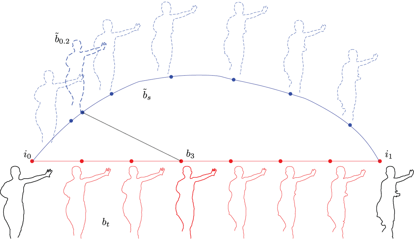
Fig. 1. Geodesic path of elastic deformations $\tilde b_s$
from the curve i
0 to i
1 (in dashed blue lines). b
3 is one of the contours b
t
extracted from the intermediate frames between the two reference ones, a good matching EC
$\tilde b_s$
from the curve i
0 to i
1 (in dashed blue lines). b
3 is one of the contours b
t
extracted from the intermediate frames between the two reference ones, a good matching EC $\tilde b_{0.2}$
along the path is highlighted.
$\tilde b_{0.2}$
along the path is highlighted.
These observations lead us to conceive a lossless coding technique for object contours: supposing that the encoder and the decoder share a representation of the initial and final shapes, they can reproduce the exactly same geodesic path between them. Then, the decoder will conveniently decide which point of the geodesic (one of the blue curves in Fig. 1) shall be used as context information to encode an intermediary contour (one of the red curve in the same figure). The encoder will only have to send a value s* ∈ [0, 1] to identify this curve. If this curve is actually similar to the one to be encoded, it is possible to exploit this information to improve the lossless coding of the latter. However, how to do this is not obvious, and the solution to this problem is one of the main contributions of this paper.
B) Lossless contour coding
Various techniques have been developed to represent and code the boundaries of objects, like polygon approximation [Reference O'Connell21] or chain coding [Reference Katsaggelos, Kondi, Meier, Ostermann and Schuster14]. The latter is the most common method to losslessly encode boundary pixels. A chain code follows the contour of an object and encodes the direction of the next boundary pixel with respect to the current one. Since an object tends to have a quite regular contour it is usually more convenient to code the change of direction with respect to the previous one, thus leading to differential chain codes. An example of differential chain coding of the 8-connected contour of an object is given in Fig. 2. The sequence of symbols produced by a chain code is fed into an entropic encoder, such as a variable length encoder or an arithmetic encoder, possibly using contexts to improve its performance [Reference Cagnazzo, Antonini and Barlaud22].
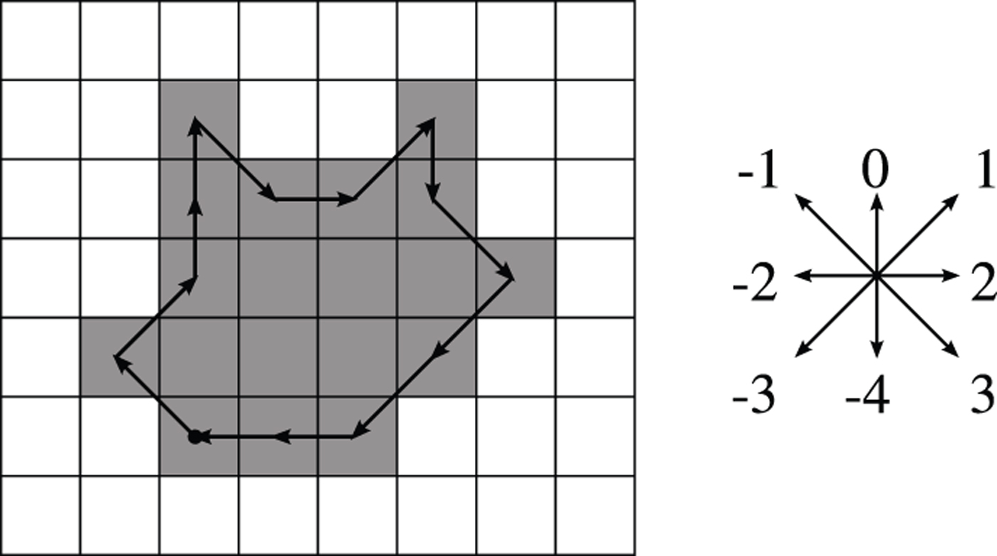
Fig. 2. Differential chain code: the arrows represent the symbols of the differential chain code if the previous symbol is “Up”. We can code the contour of the object, from the starting point, as: “Up-Left”, 2, − 1, 0, 3, − 1, − 1, 3, − 1, 2, 0, 1, 0.
Recently Daribo et al. [Reference Daribo, Cheung and Florencio17] introduced a new technique aimed at the lossless coding of edges that resulted to be the best among the others. However, it is conceived in a block-based coding environment, we retain it as a base to develop our contour-based coding technique. Their main idea is that contours of a physical object possess geometrical structures that can be exploited to predict the direction of the next symbol, given a window of consecutive previous samples. A chain code is used to represent a contour, and each symbol is encoded with an arithmetic encoder that uses a probability distribution adaptively computed using the previous symbols. The probability distribution is centered around the estimated most probable direction, which in turn is obtained using linear regression (LR) on a suitable window of previous samples: the underlying assumption is that contours exhibit linear trends. The prediction of directions and the assignment of the probability values can be reproduced at the decoder, provided that some parameter is transmitted as side information.
This method has much better performance than other popular techniques [Reference Daribo, Cheung and Florencio17], but further improvements are possible. On the one hand, the LR can be replaced with a more effective estimator for the direction of the next symbol. On the other hand, the encoding algorithm does not take advantage from temporal correlation of contours and the prediction of the most probable direction cannot cope with sudden changes of direction.
Our proposed method uses temporal correlation of contours by producing an elastic estimation of the current curve; this curve is subsequently employed for improving the statistical model of the current symbol of the chain code, resulting in a remarkable improvement of the coding rate. The two reference curves used to produce the elastic deformation are encoded using our improved version of the technique described by Daribo et al. [Reference Daribo, Cheung and Florencio17].
III. PROPOSED TECHNIQUE
We propose a technique for encoding the contour of an object in a single view video sequence, in a multiview set of images or in an MVD, and in any context where two reference curves are available. The targeted application is depth coding in MVD applications, and this for two reasons: first, contour information is extremely important for depth, and its lossless representation is necessary for obtaining a good subjective quality for synthesized views; second, extracting contours from a depth map is relatively easy, since they are typically made up of smooth regions separated by sharp discontinuities. However, in this paper, we do not investigate the contour extraction from depth images, but uniquely their lossless coding; moreover, we point out that our method can also be applied on contours extracted from natural videos, as we show in the experimental results. In this last case, contours are typically extracted from precise segmentation maps: our method efficiently encodes both contours automatically extracted from depths and contours obtained by segmentation.
As already mentioned, our method apply to the case where we have a set of contours related to the same object, be them representing the temporal evolution of the object borders or their deformation related to the change of viewpoint: the example in Fig. 1 refers to the latter case. However, without loosing generality, we consider the following use case. We have a set of K ≥ 3 contours (K = 8 in Fig. 1). We refer to the parametric representation of the first contour as i 0[n] = (x i 0 [n], y i 0 [n]), with n ∈ {1, 2, …, N i 0 }; likewise, i 1[n] with n ∈ {1, 2, …, N i 1 } is the parametric representation of the last contour, and b t [n] with n ∈ {1, 2, …, N t } the one of the generic t-th intermediate curve, with t ∈ {1, …, K − 1}. We propose an “intra method” (i.e. without temporal prediction) to encode i 0 and i 1, and a “bidirectional method” (i.e. with prediction from two already encoded curves) for the curves b t . We will refer to the intra-coded contours as “I-contours” and to the K − 2 intermediate contours, to which our prediction-based method is aimed, as “B-contours”.
Indeed, the I-contours are supposed to be available at the encoder and at the decoder before the B-contours in order to develop a prediction method to code the latter. To encode the I-contours i 0 and i 1 we propose a small yet effective modification to the technique described in [Reference Daribo, Cheung and Florencio17]. The difference between the modified and the original version lies in the predictor for the direction of the next symbol, as shown in Section IIIB.
Let us now describe the proposed method for the B-contours, the basic idea is independent from the value of K and from the structure of dependencies (or, borrowing the terms from the classical hybrid video coding paradigm, from the GOP structure). More precisely, in order to encode b t, we consider the geodesic path between i
0 and i
1. The elastic deformation tool allows us to easily generate any intermediate curve on the geodesic (dashed blue curves in Fig. 1), simply by specifying a position parameter s ∈ [0, 1]. Let us refer to $\tilde{b}_s \lsqb n\rsqb $
the parametric representation of a curve on the geodesic. We observe that
$\tilde{b}_s \lsqb n\rsqb $
the parametric representation of a curve on the geodesic. We observe that $\tilde{b}_0 = i_0$
and
$\tilde{b}_0 = i_0$
and $\tilde{b}_1 = i_1$
. Since i
0 and i
1 are available at the encoder and the decoder, they both can produce the same curve
$\tilde{b}_1 = i_1$
. Since i
0 and i
1 are available at the encoder and the decoder, they both can produce the same curve $\tilde{b}_s$
, for any s, and use it as side information for the lossless encoding of b t. Intuition suggests that the encoder and the decoder could agree in using
$\tilde{b}_s$
, for any s, and use it as side information for the lossless encoding of b t. Intuition suggests that the encoder and the decoder could agree in using $s = \displaystyle{t \over K-1}$
as the position on the geodesic used to predict b
t
. However, as we will show in the experimental section, a significant coding gain can be obtained if we let the encoder select a suitable value for s, let it be s*, and use it for the encoding. Of course, s* should be transmitted to the decoder using a suitable number of bits. The choice of s* and the number of coding bits will be discussed in the experimental section. Likewise, the problem of the optimal “GOP structure” will be discussed in Section IVD. In the rest of the current section, in order to simplify the discussion, we will consider a simple IBIBIB… configuration. This is equivalent to having K = 3: in other words, we encode an object contour knowing the previous and the future curves. The proposed method can however be applied to any value of K without major modifications. Other coding structures are shown in the experimental part at Section IVD.
$s = \displaystyle{t \over K-1}$
as the position on the geodesic used to predict b
t
. However, as we will show in the experimental section, a significant coding gain can be obtained if we let the encoder select a suitable value for s, let it be s*, and use it for the encoding. Of course, s* should be transmitted to the decoder using a suitable number of bits. The choice of s* and the number of coding bits will be discussed in the experimental section. Likewise, the problem of the optimal “GOP structure” will be discussed in Section IVD. In the rest of the current section, in order to simplify the discussion, we will consider a simple IBIBIB… configuration. This is equivalent to having K = 3: in other words, we encode an object contour knowing the previous and the future curves. The proposed method can however be applied to any value of K without major modifications. Other coding structures are shown in the experimental part at Section IVD.
In the rest of this section, we will explain how to select a suitable part of the EC $\tilde{b}_s$
to be used as context to encode the current edge symbol; how to use this information to determine the most probable direction for the next symbol on the contour; and which side information needs to be sent to the decoder such that it can replicate the same behavior as the encoder.
$\tilde{b}_s$
to be used as context to encode the current edge symbol; how to use this information to determine the most probable direction for the next symbol on the contour; and which side information needs to be sent to the decoder such that it can replicate the same behavior as the encoder.
A) Correspondence function
In this subsection, we consider the encoding of a single curve b t using the elastic representation $\tilde{b}_s^{\ast}$
, with s* suitably selected by the encoder. For the encoding of i
0 and i
1 we do not use the elastic deformation.
$\tilde{b}_s^{\ast}$
, with s* suitably selected by the encoder. For the encoding of i
0 and i
1 we do not use the elastic deformation.
The curves are sampled respectively on N
b
and $N_{\tilde b}$
points. To simplify the notation, we will drop the subscript t and s* where this does not give rise to ambiguities.
$N_{\tilde b}$
points. To simplify the notation, we will drop the subscript t and s* where this does not give rise to ambiguities.
To use the suitable portion of the synthetic curve $\tilde{b}$
as side information to code the current point on b, it is essential to have a function that associates each point of b to the corresponding point of
$\tilde{b}$
as side information to code the current point on b, it is essential to have a function that associates each point of b to the corresponding point of $\tilde{b}$
. This function is generated at the encoder and has to be transmitted to the decoder.
$\tilde{b}$
. This function is generated at the encoder and has to be transmitted to the decoder.
In order to establish an association between the two curves, we use dynamic time warping (DTW) [Reference Müller23]. First, it is needed to establish a feature space ${\cal F}$
for the curves: a distance in this space will then be used to create the DTW function. Since we want to link the parts of the curve that have the same characteristics in terms of lobes, spikes and such, we used the direction of the tangent vector as featureFootnote
1
. Let us use a complex representation that associates to every point (x, y) the complex number p = x + ȷ
y, and let us refer to the sequence of tangent vectors of the curve c = (x
c
, y
c
) as φ
c
:
${\cal F}$
for the curves: a distance in this space will then be used to create the DTW function. Since we want to link the parts of the curve that have the same characteristics in terms of lobes, spikes and such, we used the direction of the tangent vector as featureFootnote
1
. Let us use a complex representation that associates to every point (x, y) the complex number p = x + ȷ
y, and let us refer to the sequence of tangent vectors of the curve c = (x
c
, y
c
) as φ
c
:
 $$\forall n \in \lcub 1\comma \; \ldots\comma \; N_c\rcub \comma \; \varphi_{c}\lsqb n\rsqb = \arg \lpar p_{c}\lsqb n\rsqb - p_{c}\lsqb n - 1\rsqb \rpar \in {\cal F}\comma \;$$
where ${\cal F} = \lsqb -\pi\comma \; \pi\lsqb $
. Computing equation (5) for b and
${\cal F} = \lsqb -\pi\comma \; \pi\lsqb $
. Computing equation (5) for b and $\tilde{b}$
we obtain the sequences of features φ
b
and
$\tilde{b}$
we obtain the sequences of features φ
b
and $\varphi_{\tilde{b}}$
defined on N
b
and
$\varphi_{\tilde{b}}$
defined on N
b
and $N_{\tilde b}$
points, respectively.
$N_{\tilde b}$
points, respectively.
A typical behavior of two feature sequences is shown in Fig. 3; while the two sequences have similar shapes, they are not aligned. To perform the alignment we need a local distance measure (or local cost measure), defined as $d \colon {\cal F} \times {\cal F} \rightarrow \open{R}^+$
. The local distance measure d(φ
b
[n],
$d \colon {\cal F} \times {\cal F} \rightarrow \open{R}^+$
. The local distance measure d(φ
b
[n], $\varphi_{\tilde b}\lsqb m\rsqb $
) should be small when the two features are similar, large otherwise. Since in our case
$\varphi_{\tilde b}\lsqb m\rsqb $
) should be small when the two features are similar, large otherwise. Since in our case ${\cal F} \subset \open{R}$
, we can use as distance the square of the direction difference:
${\cal F} \subset \open{R}$
, we can use as distance the square of the direction difference: $\lpar \vert \varphi_{b} - \varphi_{\tilde b}\vert \, \hbox{mod} \, \pi\rpar ^{2}$
. By evaluating the local cost measure for every couple of elements in the sequences, we obtain the cost matrix
$\lpar \vert \varphi_{b} - \varphi_{\tilde b}\vert \, \hbox{mod} \, \pi\rpar ^{2}$
. By evaluating the local cost measure for every couple of elements in the sequences, we obtain the cost matrix $C \in \open{R}^{N \times M}$
, where the generic element is defined as follows:
$C \in \open{R}^{N \times M}$
, where the generic element is defined as follows:
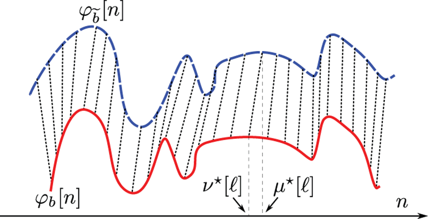
Fig. 3. Example of association of two sequences by DTW.
 $$\eqalign{C\lpar n\comma \; m\rpar & = d\lpar \varphi_{b}\lsqb n\rsqb \comma \; \varphi_{\tilde b}\lsqb m\rsqb \rpar \cr &= \lpar \vert \varphi_{b}\lsqb n\rsqb - \varphi_{\tilde b}\lsqb m\rsqb \vert \, \hbox{mod} \, \pi \rpar ^2.}$$
We have to find now the sequence ψ, defined as a sequence of couples:
 $$\psi\lsqb \ell\rsqb = \lpar \nu^\ast_\ell\comma \; \mu^\ast_\ell\rpar \in \lcub 1\comma \; \ldots\comma \; N\rcub \times \lcub 1\comma \; \ldots\comma \; M\rcub \comma \;$$
such that:
 $$\lpar \nu^\ast\comma \; \mu^\ast\rpar = \arg \nolimits {\min_{\lpar \nu\comma \mu\rpar }} \sum_{l=1}^{L} C\lpar \nu\lsqb \ell\rsqb \comma \; \mu\lsqb \ell\rsqb \rpar $$
under the conditions:
-
• boundary condition, ψ[1] = (1, 1) and ψ[L] = (N, M);
-
• monotonicity of ν*[ℓ] and μ*[ℓ];
-
• step size, ψ[ℓ] − ψ[ℓ − 1] ∈ {(0, 1),(1, 0),(1, 1)}.
In practice, ψ is a sequence of indices (ν*[ℓ], μ*[ℓ]) of the curves φ
b
and $\varphi_{\tilde b}$
, such that φ
b
[ν*[ℓ]] and
$\varphi_{\tilde b}$
, such that φ
b
[ν*[ℓ]] and $\varphi_{\tilde b}\lsqb \mu^{\ast}\lsqb \ell\rsqb \rsqb $
are best matched under the aforementioned constraints. The association by DTW of the two sequences is shown in dotted black lines in Fig. 3.
$\varphi_{\tilde b}\lsqb \mu^{\ast}\lsqb \ell\rsqb \rsqb $
are best matched under the aforementioned constraints. The association by DTW of the two sequences is shown in dotted black lines in Fig. 3.
In our application, the correspondence function obtained with DTW on the direction of the tangent vector is very close to a straight line and it can be approximated with a first-order polynomial. The approximation has two main effects: first it reduces the number of bits needed to code the function; moreover it prevents sudden variations on the correspondence function that are rather related to outliers than actual values. However, one may wonder whether it is worth computing the exact DTW only for approximating at a first order: maybe a simple rescaling of the “temporal” axis from N points to M points could be as effective as the approximated DTW, without needing to compute the correspondence function. We have dealt with this issue with a simple heuristic approach: we compared the coding rate of our algorithm in two cases: in the first, we use the first-order approximation of the DTW function; in the second we use a rescaling of N/M. We observed that using the DTW gives an average rate reduction of 5.33%. For this reason, we kept the DWT in our system.
In Fig. 4, there is an example of DTW and its linear approximation. The resulting correspondence between the points of the two curves is shown in Fig. 5. We see that all the main features of the curves are located and put in correspondence, so that for each point of the actual curve b there is an associated point on the EC $\tilde{b}$
, whose neighborhood is the side information we want to use to enhance the coding of b.
$\tilde{b}$
, whose neighborhood is the side information we want to use to enhance the coding of b.
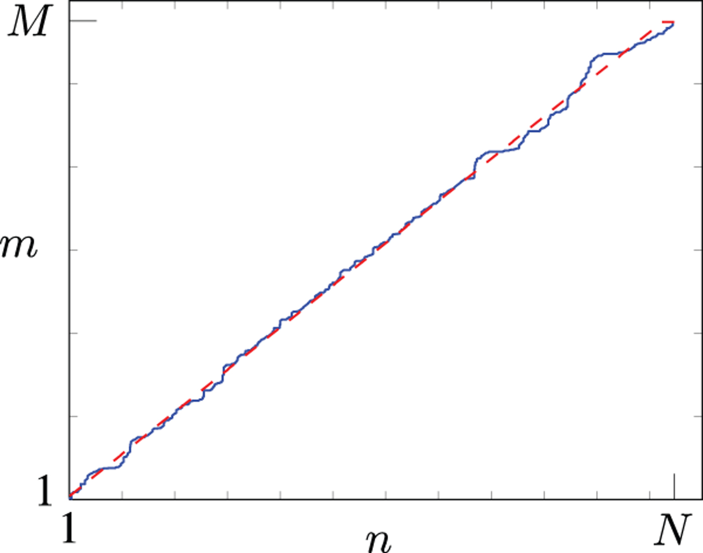
Fig. 4.
Ballet: correspondence function. In blue the association of the two curves using the DTW of the direction of the tangent vector, in dashed red the approximation with a first-order polynomial, whereas n and m are the indices of samples on the curves b and $\tilde{b}$
, respectively.
$\tilde{b}$
, respectively.
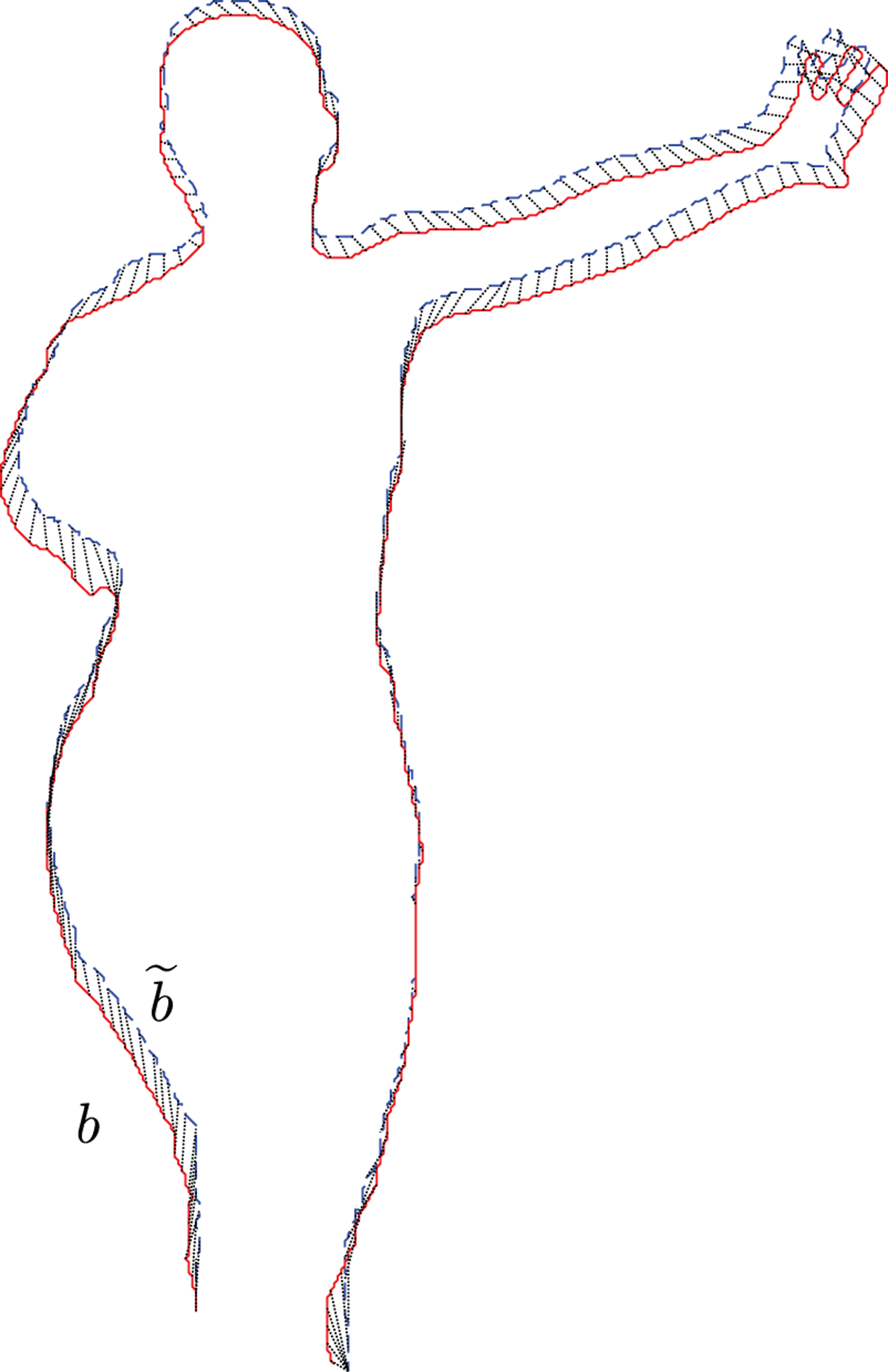
Fig. 5.
Ballet: correspondences between the EC $\tilde{b}$
(dashed blue) and the curve to code b (red).
$\tilde{b}$
(dashed blue) and the curve to code b (red).
B) Context
The correspondence function allows us to associate the current point to a portion of the EC, centered in the corresponding point. This information is used as side information to have more accurate probability values for the next symbol. We called this information the context, and for each point of the curve b, it is composed by:
-
• v 0, a vector of N 0 points of the curve b transmitted so far (in red in Fig. 6);
-
• v 1 p : the “past” on the EC (in dashed blue in Fig. 6), a vector of N p points of $\tilde{b}$
corresponding to v
0; more precisely, v
1 p
is constituted of the points between those corresponding to the terminal points of v
0;
$\tilde{b}$
corresponding to v
0; more precisely, v
1 p
is constituted of the points between those corresponding to the terminal points of v
0; -
• v 1 f : the “future” on the EC, a vector of N f points of the EC
$\tilde{b}$
following the current correspondent point on
$\tilde{b}$
(in dark blue in Fig. 6).


Fig. 6. Extracts from the curves b (red) and $\tilde{b}$
(dashed blue). The correspondences between the two curves are indicated with thin dotted black lines. The dashed lines represent the extracted direction for the vectors of points v
0, v
1 p
, and v
1 f
.
$\tilde{b}$
(dashed blue). The correspondences between the two curves are indicated with thin dotted black lines. The dashed lines represent the extracted direction for the vectors of points v
0, v
1 p
, and v
1 f
.
Of course v 1 p and v 1 f are only available for B-contours, for I-contours only v 0 is available. We use the context to obtain the most probable direction for the next symbol, then we use this result to define a distribution using the von Mises statistical model [Reference Mardia and Jupp24].
1. Direction extraction
For all the set of points of the different curves, we have to estimate the direction of the next symbol. In the case of the I-contours, only the set of points p 0 are used, whereas in the case of B-contours all the three sets of points v 0, v 1 p , and v 1 f are used.
Several approaches can be used to extract a direction from a set of ordered points. E.g. in [Reference Daribo, Cheung and Florencio17] an LR on v 0 is used. We found that a simple average direction (AD) is even more effective. Using the same complex representation as in IIIA, the estimated direction α can be obtained using the following formula:
 $$\alpha \lpar {\bf v} \rpar = \arg\left(\displaystyle{1 \over N-1} \sum_{n=2}^{N}\lpar {\bf v}\lsqb n\rsqb - {\bf v}\lsqb n - 1\rsqb \rpar \right)\in \lsqb -\pi\comma \; \pi\rsqb \comma \;$$
where v is the complex representation of a generic vector of N points, and is defined as v = [x 1 + ȷ y 1, x 2 + ȷ y 2, …, x N + ȷ y N ]; arg is the argument of a complex number.
2. Most probable direction
Applying α on the complex representation of v
0, we obtain α0, the angle of the AD based solely on the previously transmitted samples. Likewise, α1 p
and α1 f
are the ADs based on the vectors v
1 p
and v
1 f
of the curve $\tilde{b}$
. We develop a method to estimate θ, the most likely direction of next symbol of b: we use α1 f
to adjust the direction α0. In this way, we manage to seize the sudden changes and go along the long trends.
$\tilde{b}$
. We develop a method to estimate θ, the most likely direction of next symbol of b: we use α1 f
to adjust the direction α0. In this way, we manage to seize the sudden changes and go along the long trends.
A simple and intuitive formula to take into account the context for the prediction of the most probable direction is:
 $$\theta = \lpar 1 - q\rpar \alpha_0 + q \alpha_{1 f}\comma \;$$
with q ∈ [0, 1]. This way we can weight the directions of the past of the curve b and the future of the curve $\tilde{b}$
. To decide the weight q, we observe that the side information of the EC is not essential when the curves are regular, while it becomes fundamental next to the occurrence of a sudden change. So q should be small if for the current point the directions extracted from the two curves are similar (so that θ is close to α0), and close to 1 if they are not (so that θ close to α1 f
):
$\tilde{b}$
. To decide the weight q, we observe that the side information of the EC is not essential when the curves are regular, while it becomes fundamental next to the occurrence of a sudden change. So q should be small if for the current point the directions extracted from the two curves are similar (so that θ is close to α0), and close to 1 if they are not (so that θ close to α1 f
):
 $$q = \displaystyle{{\max \lcub \vert \alpha_0 - \alpha_{1 p}\vert \comma \; \vert \alpha_0 - \alpha_{1 f}\vert \rcub }\over{\pi}}.$$
The value of q is related to the modulus of the difference of directions, and it is large if α0 is very different from α1 p or α1 f because a dissimilarity in the neighborhood of the current point suggests a change which is not predicted solely from α0.
3. Adaptive statistical model
We retain the statistical model described in [Reference Daribo, Cheung and Florencio17] to assign values to the symbols for the next edge. It is based on the von Mises distribution and the distribution parameters are set according to the information extracted from the curves b and $\tilde{b}$
. The von Mises distribution is the Gaussian distribution for angular measurements and it is defined as [Reference Mardia and Jupp24]:
$\tilde{b}$
. The von Mises distribution is the Gaussian distribution for angular measurements and it is defined as [Reference Mardia and Jupp24]:
 $$p\lpar \beta\vert \mu\comma \; \kappa\rpar = \displaystyle{{e^{\kappa \cos\lpar \beta - \mu\rpar }} \over {2 \pi I_0\lpar \kappa\rpar }}\comma \;$$
where I 0(·) is the modified Bessel function of order 0, μ is the mean and in this case it coincides with the estimated direction θ, 1/κ is the variance of the distribution. As in [Reference Daribo, Cheung and Florencio17], we set κ as a function of the predicted direction θ: when θ is aligned with the axis of the pixel connection grid, intuition tells us that it is more convenient to give a higher probability value to the symbol that represents that direction. So κ is set to:
 $$\kappa = \rho \cos\lpar 2\hat{\theta}\rpar \comma \;$$
where $\hat{\theta} = \min\lcub \vert \theta - \gamma_{i}\vert \rcub $
, and γ
i
are the angles of the pixel connection grid (
$\hat{\theta} = \min\lcub \vert \theta - \gamma_{i}\vert \rcub $
, and γ
i
are the angles of the pixel connection grid ( $\left\{0\comma \; \displaystyle{\pi\over 8}\comma \; \displaystyle{2\pi\over 8}\comma \; \ldots \right\}$
in the case of an eight-connected grid). The parameter ρ represents a “confidence level” of the prediction: as it grows it makes the distribution more unbalanced, so the more precise is the prediction based on the context, the larger it should be to achieve higher coding gains.
$\left\{0\comma \; \displaystyle{\pi\over 8}\comma \; \displaystyle{2\pi\over 8}\comma \; \ldots \right\}$
in the case of an eight-connected grid). The parameter ρ represents a “confidence level” of the prediction: as it grows it makes the distribution more unbalanced, so the more precise is the prediction based on the context, the larger it should be to achieve higher coding gains.
C) Coding
The curve b, represented with a differential chain code, is encoded with an arithmetic coder which for each symbol uses the probability vector assigned by the adaptive statistical model. The encoder needs to transmit to the decoder the parameters involved in the coding process:
-
• s*, the selected point on the geodesic path;
-
• the correspondence function, approximated by a first-order polynomial, so two parameters;
-
• the parameter ρ;
-
• N 0 and N f .
With this information the decoder can reproduce the behavior of the encoder and it will compute the same probability values for each point of the curve b. We observe that N p does not need to be sent, since it is deduced by applying the correspondence function to v 0.
IV. EXPERIMENTAL RESULTS
The proposed method has been evaluated using the multiview sequences ballet (provided by Microsoft Research), mobile (Philips), lovebird (ETRI/MPEG Korea Forum), and beergarden (Philips). We encoded the curves corresponding to the main object in the depth sequences for a fixed time instant or view. We used to test our algorithm also masks extracted from the standard monoview sequences stefan and foreman.
The curves for ballet, mobile, lovebird, and beergarden depths were obtained using the Canny edge detector [Reference Canny25]. Depth maps are not as complex as texture images and the use of the Canny edge detector produced very good results in our test cases. We extracted the contours of very precise segmentation maps for the sequences stefan [Reference Chen, Bajić and Saeedi26, Reference Chen and Bajić27] and foreman [28]. This latter case can be seen as the ideal test case.
The coding scheme concentrates almost all the computational load at the encoder side. In particular, for the B-contours the choice of the values of (N p , N f , ρ, s) can be simply made trying out every possible combination and selecting the one that gives the best outcome. This full search method, however optimal, is extremely costly in terms of time and complexity. We thus introduced a greedy algorithm that optimizes one variable at a time to find a sub-optimal solution.
A) Coding of I- and B-contours
To code the I-contours we replaced the LR with the more effective AD in the technique described in [Reference Daribo, Cheung and Florencio17], whereas for the coding of the B-contours we can take advantage of the context provided by the ECs, thus achieving better coding gains. In Table 1, are shown the results for a set of images taken from the test sequences. We notice that just altering the direction extraction method from LR to AD the average coding cost is reduced by 4.88%, while passing from AD to AD with EC context leads to a reduction of 1.82%, for a total reduction of 6.53%. If on the other hand we use the LR with the EC context, then the rate reduction is 2.25%.
Table 1. Coding results (in bits) for the different contributions of the developed tools to the technique proposed in [Reference Daribo, Cheung and Florencio17], applied to object contours. Two different methods to extract the probable direction from a set of points: linear regression (LR), and average direction (AD), without and with elastic curve (EC) context.
B) Side information cost
We will now account for the cost to transmit the four parameters s*, N p *, N f *, and ρ*, as well as the correspondence function.
The correspondence function is the result of a linear approximation and experiments show that using 10 bits to code the two parameters of the straight line leads to the same performance as coding them with double precision.
For N p * and N f * we decided to use 1 bit for the range of N p ({5, 6} ), and 2 bits for the range of N f ({6, 7, 9, 11} ), once again based on experimental results. On the other hand, the optimal ρ has a wider range of values, and we observed that typical values can be represented by the set {6.6 + kΔ}, with Δ = 0.1 and k = 0, …, 31, for a cost of 5 bits.
We observe that the accuracy of the representation of the position on the geodesic s* has a quite large influence on the coding efficiency. Using for example 2 bits to code the possible positions we have four curves to use as side information to code the curve b, using 3 bits leads to eight curves, in general using a fixed length representation with b s bits permits us to choose among 2 b s different curves. The chance of finding a good matching curve to use as a side information increases with b s , but for every bit added the complexity doubles, and we are increasing the cost of the representation too. If some values are more probable than others it is worth to consider a variable length code to reduce the cost of the representation.
We thus used an experimental approach and compared two different ways to code s*: a fixed length coding, with length from 2 to 10, and an Exponential-Golomb code. In Table 2, we see that, performing the average on different curves and on different sequences, a fixed length coding leads to better performance if the number of bits used for the representation of s* approaches to 6 or more. To compare the proposed method to other techniques we choose the best performing 10 bits fixed length coding.
Table 2. Average coding cost (in bits) for different ways of coding s*: fixed length coding up to 10 bits and Exp-Golomb.

For the I-contours we only have to transmit as side information the parameters N p * and ρ*, corresponding to an overall cost of 6 bits. On the other hand, the decoding of the B-contours needs the correspondence function as well as the four parameters N p *, N f *, ρ*, and s*, corresponding to an overall cost of 28 bits.
C) Greedy algorithm (GA)
Resting on experimental results for each variable we selected a range of typical values. We initialize the GA with a starting point (N p0, N f0, ρ0, s 0), corresponding to the solution in which every value is the closest to the center of the coded range, and then the GA optimizes the variables in the order N p , N f , ρ, s. Keeping fixed N f0, ρ0, and s 0 the GA runs the proposed technique to select the N p that minimizes the bit rate. Once N p * has been found the algorithm starts again to optimize N f from the point (N p *, N f0, ρ0, s 0). Then again for ρ and s, until it reaches the solution (N p *, N f *, ρ*, s*).
The search order for the parameters is set according to our observations of the optimum parameter distributions after the full search for many sequences: N p * has a very peaked distribution, so the selected value after the first step of the GA should actually be the best one. N f *, on the contrary, has an almost uniform distribution, thus making difficult to locate the best value; it is however required to select it before ρ*, because the best value of ρ is influenced by the selected values of N p and N f . Still based on our observations, the last parameter to select is s.
As we can see in Table 3, the average loss with respect to the full search is 0.82%, but the number of calculations the encoder has to do is approximately reduced by a factor of 250.
Table 3. Average coding cost (in bits) for the full search and the greedy algorithm (GA).
Regarding the overall time needed for the coding of a curve, we can distinguish fixed and variable time contributions. The elastic estimation is fixed but we can decide how many frames to leave in between the two reference ones. On the other hand, the execution time for the choice of the parameters can vary greatly: a full search is very costly, and even if the GA speeds up the whole process, one can also decide to keep the same parameters (or a subset of the parameters) for a certain number of frames.
D) Comparisons
We compare our technique to various methods to code the differential chain code of the contours: Adaptive Arithmetic Coder (AAC), Context Based Arithmetic Coder (CBAC), and the technique proposed in [Reference Daribo, Cheung and Florencio17].
In the compression of B-contours, we achieve gains up to 10% compared to the method of [Reference Daribo, Cheung and Florencio17], but to make a fair comparison we have to consider for our technique both I-contours and B-contours of the GOP structure. To study the influence of the GOP structure on the coding performance we used the following:
-
• IBIBIB … is very effective for the B-contours, since the two reference frames are very close and the prediction is very accurate, but the I-contours have a non negligible cost on the final outcome. Using this GOP structure produced in our experiments an average bit rate of 1000,19 bits per contour;
-
• IBBIBB … and IBBBIBBB … are flat structures with fairly distant I-contours, they produced an average bit rate of 1004.03 and 1010.28 bits per contour, respectively;
-
• I1B1B2B3I2 … is a hierarchical structure with 5 frames in the GOP, in which B2 is predicted using I1 and I2, B1 using I1 and B2, and so on. It produced an average bit rate of 997,57 bits per contour.
The hierarchical structure proved to be the most effective GOP structure: the cost of the I-contours is low and the elastic prediction for B2 is just slightly less accurate than the ones for B1 and B3. This result is expected, given the previous study on depth map compression with traditional hybrid techniques that shows the importance of the prediction order [Reference Maugey and Pesquet-Popescu29].
In Table 4, the average results for the test sequences are shown, and in every case our technique performs better than the others. The overall average gain with respect to the second best coding technique in the group, the one proposed in [Reference Daribo, Cheung and Florencio17], is 6.53%. If we consider instead the gain of the proposed technique with respect to JBIG2, which is not optimized for this kind of data but has been chosen to code the boundary information in [Reference Gautier, Le Meur and Guillemot8], it is 65.09%. Over other standard techniques, such as AAC and CBAC (with one symbol context, the best choice in our tests) the average gains are of 23.93 and 18.06%, respectively.
Table 4. Average coding cost (in bits) for various sequences in the view domain (ballet) and in the time domain (mobile, lovebird, beergarden, stefan). The tested methods are: JBIG2, Adaptive Arithmetic Coder (AAC), Context Based Arithmetic Coder (CBAC) with 1 symbol context, the one proposed in [Reference Daribo, Cheung and Florencio17], and the proposed technique (all the side information cost accounted). In the last column are reported the gains of the proposed technique over the other best performing one in the group.
E) Object-based depth maps coding technique
We underline here that the goal of this paper is not to propose a complete system for MVD coding, but only to show the potential of the lossless contour coding based on elastic deformation. In this respect, we show that a relatively simple codec based on this tool may be competitive with (or even better than) the state of the art and this may be considered a validation of the proposed approach.
Coming to the implementation, we observe that it is very difficult to integrate our object-based technique into a 3DVC coder. We resort to an existing object-based technique since it can immediately benefit from an improved contour coding method, even though it is not the best option from an rate-distortion (RD) perspective. Despite the simplicity of the approach, as we will show, we have satisfying results, due to the nature of the data we want to compress. In summary, the new object-based compression technique is composed of:
-
• the proposed technique for the contours of the object with a hierarchical GOP structure I1B1B2B3I2, as described in Section IVD. This part provides a lossless coding with inter-frame prediction;
-
• for the inner part of the objects we use the Shape Adaptive (SA) Wavelet Transform, followed by SA Set Partitioning In Hierarchical Trees (SPIHT), followed by an arithmetic coder [Reference Cagnazzo, Poggi, Verdoliva and Zinicola30]. We remark that for the inner part of the objects we thus have an entirely “Intra” technique.
We have chosen this technique because it is reasonable and simple, and it complements perfectly with our lossless coding technique.
To make a meaningful comparison we used HEVC Intra to compress the depth maps. We believe that the comparison is fair because in the case of HEVC Intra the arithmetic coder for the lossless coding part take advantage of the context updating, and there is no temporal prediction. Likewise, in our technique, the lossless coding part exploits the temporal redundancy, while the object coding is totally “Intra”. Moreover, it would not be fair to make a comparison with HEVC Inter because we have no temporal prediction for the objects, neither would be easy to develop an object-based coder with temporal prediction.
Once defined the compression technique, we use the decoded depths to synthesize new views and make a comparison with the images generated by the uncompressed depth maps. Given any two adjacent views of the multiview sequence, we generated three equally spaced synthetic intermediate views. To test our depth maps compression technique we used the multiview sequences ballet, beergarden, lovebird and mobile, synthesizing 6, 15, 30, and 54 frames, respectively. In order to assess the quality of the virtual views, we compared them to synthesized images obtained by applying the same DIBR algorithm to the uncompressed depths and views, and thus we obtained the RD points related to our techniques and to HEVC Intra.
Finally, we computed the Bjontegaard metrics [Reference Bjontegaard31] on these RD points: we observed that our technique outperforms the reference for ballet, beergarden and mobile, achieving respectively +2.6 dB, +0.16 dB and +0.88 dB, while the PSNR was practically identical for lovebird. These results, however, pertinent to quite specific test conditions (PSNR of synthesized images, limited range), show that our technique can perform at least as well as HEVC Intra, or even better depending on the sequence: these results imply that the proposed approach is worth considering. This is even more relevant in sight of the fact that in general, object-based coding techniques achieve not very good results in image compression. It has been shown that the cost of lossless contour coding is one of the elements that undermine these techniques the most [Reference Cagnazzo, Parrilli, Poggi and Verdoliva10].
V. CONCLUSIONS
In this paper, we have proposed a new technique for lossless coding of object contours for MVD. Using elastic deformation between two reference contour curves, we obtained a useful side information for the coding of the actual contour. The price payed with the coding cost for the side information is fully rewarded with significant gains with respect to the reference techniques and to the state of the art. We have also improved the technique described in [Reference Daribo, Cheung and Florencio17] by substituting its prediction method with the AD method.
Moreover, a simple object-based depth map coding technique has been set up, showing that this approach can give interesting results, even if compared to state-of-the-art techniques, such as HEVC Intra.
So far, only a monodimensional elastic interpolation has been considered, but we expect a more precise estimation if we can take into account four or eight reference curves from different views and different times, thus leading to further improvements of the technique. This will be the subject of further study.
Marco Calemme received a BSc degree (2007) and a MSc degree (2012) in Telecommunication Engineering from Federico II University, Napoli, Italy. Since 2012 he is pursuing a Ph.D. within the multimedia group at Telecom Paristech in Paris, France. His current research interests include video coding, compression and multiview synthesis.
Marco Cagnazzo (SM'11) obtained the Laurea (equivalent to the M.S.) degree in Telecommunication Engineering from Federico II University, Napoli, Italy, in 2002, and the Ph.D. degree in Information and Communication Technology from Federico II University and the University of Nice-Sophia Antipolis, Nice, France in 2005. He was a post-doc fellow at I3S Laboratory (Sophia Antipolis, France) from 2006 to 2008. Since February 2008 he has been Maître de Conférences (roughly equivalent to Associate Professor) at Institut Mines-Telecom, Telecom ParisTech (Paris), within the Multimedia team. He is author of more than 90 contributions in peer-reviewed journals, conferences proceedings, book chapters and standardization documents. His research interests are three-dimensional video communication and coding, distribued video coding, multiple description coding, video delivery over MANETs, network coding. Dr. Cagnazzo is an Area Editor for Elsevier Signal Processing: Image Communication and Elsevier Signal Processing. Moreover he is a reviewer for major international scientific reviews (IEEE Trans. Multimedia, IEEE Trans. Image Processing, IEEE Trans. Signal Processing, IEEE Trans. Circ. Syst. Video Tech., Elsevier Signal Processing, Elsevier Sig. Proc. Image Comm., and others) and conferences (IEEE ICIP, IEEE ICASSP, IEEE ICME, IEEE MMSP, EUSIPCO, and others).
Béatrice Pesquet-Popescu (SM'06, F'13) received the engineering degree in telecommunications from the “Politeh- nica” Institute in Bucharest in 1995 (highest honours) and the Ph.D. degree from the Ecole Normale Supérieure de Cachan in 1998. In 1998, she was a Research and Teaching Assistant with Université Paris XI, Paris. In 1999, she joined Philips Research France, Suresnes, France, where she worked for two years as a Research Scientist, then as a Project Leader, in scalable video coding. Since Oct. 2000 she is with Telecom ParisTech (formerly, ENST), first as an Associate Professor, and since 2007 as a Professor, Head of the Multimedia Group. She is the Head of the UBIMEDIA common research laboratory between Alcatel-Lucent and Institut Telecom. Her current research interests are in source coding, scalable, robust and distributed video compression and sparse representations. Dr. Pesquet-Popescu was an EURASIP BoG member (2003-2010), and an IEEE Signal Processing Society IVMSP TC member and MMSP TC associate member. She serves as an Associate Editor for IEEE Signal Processing Magazine, IEEE Trans. on Image Processing, IEEE Trans. on Multimedia, IEEE Trans. on CSVT, Elsevier Image Communication, and Int. J. Digital Multimedia Broadcasting journals and was till 2010 an Associate Editor for Elsevier Signal Processing. She was a Technical Co-Chair for the PCS2004 conference, and General Co-Chair for IEEE SPS MMSP2010, EUSIPCO 2012, and IEEE SPS ICIP 2014 conferences. Beatrice Pesquet-Popescu is a recipient of the “Best Student Paper Award” in the IEEE Signal Processing Workshop on Higher-Order Statistics in 1997, of the Bronze Inventor Medal from Philips Research and in 1998 she received a “Young Investigator Award” granted by the French Physical Society. She holds 23 patents in wavelet-based video coding and has authored more than 250 book chapters, journal and conference papers in the field. In 2006, she was the recipient, together with D. Turaga and M. van der Schaar, of the IEEE Trans. on Circuits and Systems for Video Technology “Best Paper Award”. In 2012, she was “Associate Editor of the Year” for IEEE Trans. on Circuits and Systems for Video Technology.


 Open access