


Regression discontinuity (RD) is a useful tool for causal inference in natural settings. The idea is simple. When a treatment is assigned based on a threshold, cases barely below the threshold are approximately identical in all respects to those barely on the other side of the threshold. Thus, untreated cases near the threshold can serve as counterfactuals for treated cases near the threshold, and researchers can estimate a local average treatment effect with minimal assumptions. RD has an important place in the analysis of two-candidate elections since very close elections on each side of the 50 percent vote threshold are similar in all aspects except for a virtual coin flip for who wins. If its assumptions are met, RD allows causal inference regarding the consequences of a party winning versus losing on its possible incumbency advantage in later elections (e.g., Lee Reference Lee2008; Erikson and Titiunik Reference Erikson and Titiunik2015) or outcomes of elections for other offices (Folke and Snyder Reference Folke and Snyder2012; Erikson, Folke, and Snyder Reference Erikson, Folke and Snyder2015).
Yet the validity of RD for causal inference has come under challenge. An influential and award-winning article,Footnote 1 Caughey and Sekhon (Reference Caughey and Sekhon2011a), sounds a warning about the validity of the RD design when applied to US House elections in the postwar era. This article (hereafter CS) notes an interesting oddity in the distribution of outcomes for very close elections—elections within a margin of 0.5 percentage points of vote for the incumbent party.
The purpose of this letter is to show that, contrary to the impression one might get from a first reading of CS, there are no observable differences in covariates between barely winning and barely losing incumbent party candidates that could account for the lopsided incumbent party win rate. Additionally, any differences in observable variables between elections barely won by Democrats and those barely lost by Democrats vanish conditional on which party is the incumbent party.Footnote 2 This fact rules out incumbent party prowess at exploiting variables that are measured here as the source of the CS incumbent party win rate oddity.
1 Lopsided Incumbent Party Win Rate
CS shows that in very close House elections from the postwar era, those in which the incumbent party received a two-party vote share between 49.25 and 50.25 percent, the incumbent party candidate won more often than would be expected by chance.Footnote 3 In the 85 elections in this narrow range, the incumbent party won 59 times and the challenger party only 26.Footnote 4 CS speculates that incumbent parties might have some unidentified source of leverage over the opposition that allows them to boost their candidate over the finish line when (and only when) the contest is known to be very close.
The CS result has been unsettling, in part because of its seeming implausibility,Footnote 5 and in part because of its potential impact on RD analysis of elections. Eggers et al. (Reference Eggers, Folke, Fowler, Hainmueller, Hall and Snyder2015) shows that the same anomaly is not found elsewhere in legislative elections around the world, nor in other US elections, including US House elections before 1945. Eggers et al. (Reference Eggers, Folke, Fowler, Hainmueller, Hall and Snyder2015) suggests that the CS finding is a “fluke.” But if a fluke, what kind of fluke is it? Did CS identify an unexpected causal dynamic that is in operation only for modern US House elections? Or is it just a statistical anomaly, a “statistically significant” pattern that could readily be found by chance when searching over many legislatures?
CS presents evidence that appears to tilt the verdict strongly toward a newly discovered but unexpected electoral dynamic rather than a statistical fluke. Their Figure 2 (p. 394) shows that when the vote is measured as percent Democratic, instead of percent for the incumbent party, there is a clear imbalance in familiar covariates, such as previous experience in office and proportion of campaign spending by the Democrat. That is, variables that are associated with Democratic wins are more associated with Democratic wins than losses at the threshold. Since the incumbency advantage for US House elections is usually estimated with Democratic voting (not incumbent party voting) as the running variable, it would seem that the key assumptions of RD are seriously violated for estimating the incumbency advantage with RD. The control and treatment groups are not equivalent.
2 A Covariate Imbalance?
We show that what appears to be imbalance across many different things is actually only imbalance across one thing—incumbent party status. Because of the lopsided incumbent party win rate (the oddity to be explained), bare Democratic winners are more likely to be from districts previously held by Democrats (and so they are generally incumbents themselves), and bare Democratic losers are more likely to be from districts previously held by Republicans (and so they are generally challengers). Therefore, to compare bare Democratic winners to bare Democratic losers is to compare bare incumbent party winners to bare challenger losers. Because incumbents are different from challengers in many ways related to strength in the previous and present elections, this one imbalance in incumbent party status causes all of the others to appear. That is, the distributional imbalance in incumbent party vote share accounts for all of the covariate imbalance across bare Democratic winners and losers in Caughey and Sekhon’s Figure 2!
Indeed, conditioning on which party is the incumbent party makes all of the observed imbalances between bare Democratic winners and bare Democratic losers disappear. Using the CS data (Caughey and Sekhon Reference Caughey and Sekhon2011b), our Figures 1 and 2 replicate the tests in CS Figure 2 separately for elections in which the Democrats are the incumbent party and Republicans are the incumbent party, respectively.Footnote 6 Footnote 7 With the possible exception of partisan swing in the case of elections with Democratic party incumbents, there are no statistically distinguishable differences between bare Democratic winners and losers when the Democrats are the incumbent party nor between bare Democratic winners and losers when the Republicans are the incumbent party. Of course, conditioning on which party is the incumbent does not eliminate the possibility that some unobserved confounder is still imbalanced within these groups. But any such confounder is not only unmeasured but also does not result in imbalance in the variables we have measured.

Figure 1. Balance plot for Democratic winners and losers in elections in which the Democratic candidate’s relative margin was within 0.50 percentage points (led or lost by less than 0.5 percent) and the Democrats were the incumbent party.

Figure 2. Balance plot for Democratic winners and losers in elections in which the Democratic candidate’s relative margin was within 0.50 percentage points (led or lost by less than 0.5 percent) and the Republicans were the incumbent party.
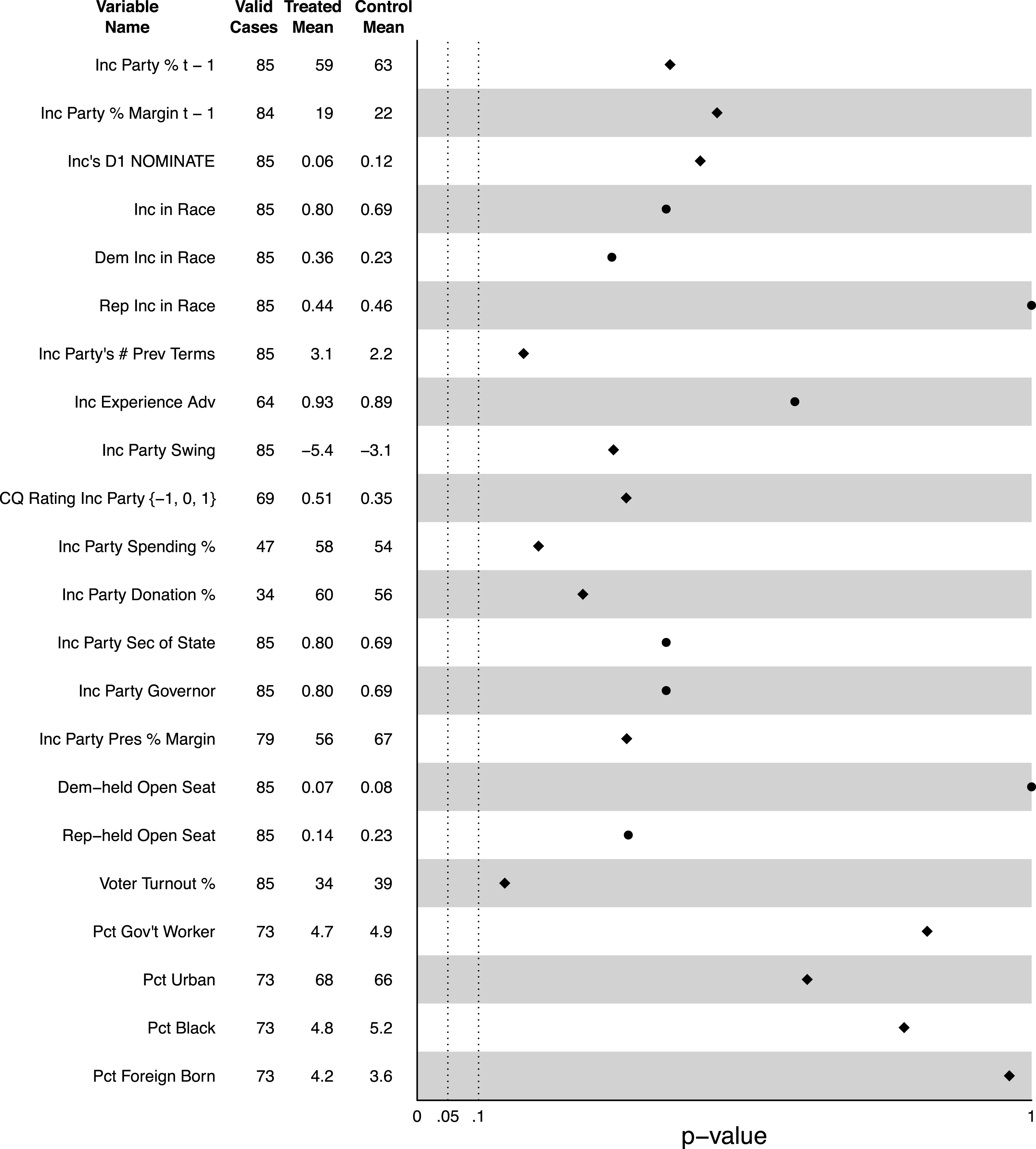
Figure 3. Balance plot for incumbent party winners and losers in elections in which the incumbent party candidate’s relative margin was within 0.50 percentage points (led or lost by less than 0.5 percent).
We can also rearrange the data to estimate the imbalance at the threshold for the incumbent party vote for all cases, combining Republican- and Democrat-held seats. Figure 3 shows that they are not statistically distinguishable on any observables in the CS dataset. Incumbent party candidates who barely win did not have substantially larger wins in the previous election than did incumbent party losers. Bare incumbent party winners do not differ ideologically from their losing counterparts. They are not more or less likely to be in a race with an actual incumbent from either party (as opposed to an open seat). They have not served more terms, nor do they have a substantial experience advantage. They are not more or less affected by national partisan swings. Their races are not more or less predictable by CQ. They do not spend more money or raise more money relative to their opponents than do their barely losing counterparts relative to their opponents. They are not more likely to share a party with their governor or secretary of state. They are not more likely to run in open seats previously held by either party. Their districts’ presidential voting is no different. They do not run in higher or lower turnout elections, and their constituents are not demographically different. In short, while incumbent party candidates have won more close elections in the postwar era than they have lost, those who win are not statistically distinguishable from those who lose. If incumbent party candidates do indeed have special leverage to push themselves over the edge in very close elections, that leverage does not manifest itself in terms of any observed imbalance herein across those who use it successfully and those who fail. To be clear, we are not arguing that we have shown that such special leverage does not exist. But our findings do suggest that the source of such leverage, if it exists, is probably outside the realm of measurable variables.
3 If No Fluke
We have argued that the disproportionate winning record of incumbent candidates when the vote is very close to the 50–50 threshold is implausible as more than just a statistical “fluke.” To call it a fluke is to assert the absence of sorting at the threshold—to deny that when close to the threshold, some candidates have a special ability to manipulate themselves onto the winning side. But what if our assertion is incorrect? In particular, what exactly would be the consequences for using RD to estimate the incumbency advantage?
The confounding condition would be that some candidates, mainly incumbents, have a unique ability to exert the necessary effort for a final spurt to win very close elections. This same unmeasured endowment could also operate to distort the vote in the next election, at $t+1$
. Consider then an RD analysis to estimate the
$t+1$
. Consider then an RD analysis to estimate the $t+1$
incumbency advantage by comparing districts where the incumbent barely wins and where the incumbent barely loses in election
$t+1$
incumbency advantage by comparing districts where the incumbent barely wins and where the incumbent barely loses in election $t$
in terms of their party’s performance in election
$t$
in terms of their party’s performance in election $t+1$
. It would be easy to imagine that if barely winning incumbents at time
$t+1$
. It would be easy to imagine that if barely winning incumbents at time $t$
are exceptionally strong candidates, the estimate of the
$t$
are exceptionally strong candidates, the estimate of the $t+1$
incumbency advantage would be biased upwards.
$t+1$
incumbency advantage would be biased upwards.
What would be the remedy? A simple solution known as “donut RD” would be to exclude the potentially offending cases closest to the threshold and conduct an RD predicting the $t+1$
vote from the incumbent vote running variable plus passing the threshold (Almond and Doyle Reference Almond and Doyle2011; Barreca, Lindo, and Waddell Reference Barreca, Lindo and Waddell2016). As Barreca, Lindo, and Waddell (Reference Barreca, Lindo and Waddell2016) states, “dropping observations in the immediate vicinity of the treatment threshold should be thought of as a useful robustness check that has the potential to highlight misspecification in any RD design.” The statistical justification would be the assumption of the continuation of the functional form in the vicinity of the threshold.
$t+1$
vote from the incumbent vote running variable plus passing the threshold (Almond and Doyle Reference Almond and Doyle2011; Barreca, Lindo, and Waddell Reference Barreca, Lindo and Waddell2016). As Barreca, Lindo, and Waddell (Reference Barreca, Lindo and Waddell2016) states, “dropping observations in the immediate vicinity of the treatment threshold should be thought of as a useful robustness check that has the potential to highlight misspecification in any RD design.” The statistical justification would be the assumption of the continuation of the functional form in the vicinity of the threshold.
To visualize this setup, Figure 4 uses the CS data to predict the $t+1$
vote from the time
$t+1$
vote from the time $t$
vote differential (incumbent party minus the opposition), averaged within bins with the narrow width of half a percentage point. The key observations are the two bins nearest to the threshold. We could estimate the incumbency advantage using only the difference in the
$t$
vote differential (incumbent party minus the opposition), averaged within bins with the narrow width of half a percentage point. The key observations are the two bins nearest to the threshold. We could estimate the incumbency advantage using only the difference in the $t+1$
vote for these two bins. Or we could summarize the data with a regression equation predicting the
$t+1$
vote for these two bins. Or we could summarize the data with a regression equation predicting the $t+1$
vote from the time
$t+1$
vote from the time $t$
vote plus an indicator variable for the incumbent party winning at time
$t$
vote plus an indicator variable for the incumbent party winning at time $t$
. Or, as suggested above, we could perform the regression while omitting the two bins closest to the threshold.Footnote
8
$t$
. Or, as suggested above, we could perform the regression while omitting the two bins closest to the threshold.Footnote
8

Figure 4. Mean incumbent party vote margin within 0.50 bins.
It is evident that when applied to the Caughey–Sekhon data, any of these three methods would yield similar estimates of the incumbency advantage.Footnote 9 This similarity should help to assuage concern that the observational imbalance at the threshold might present a problem for estimating the incumbency advantage. If we were still worried, we could use the estimate that omits the questionable observations near the threshold.
4 The Bottom Line
Let us return to the central question about the lopsided incumbent win rate. Is it evidence of a real causal process governing postwar US congressional elections or is it something to be ignored as a statistical fluke? Our reanalysis shows that one cannot separate incumbent winners and losers based on district or candidate attributes. Thus it is highly unlikely that incumbent parties, disproportionately successful in close elections, use measurable covariates to push themselves over the finish line. By elimination, any special resources that give a true advantage for the incumbent party in close elections must be intangible incumbent party assets that are not measured here. Although we cannot be certain that what cannot be observed does not exist, the absence of a covariate imbalance in terms of observable variables pushes the verdict in the direction of fluke rather than causal process.
If it is a fluke, the tendency for the incumbent party to win very tight elections would not matter for using RD to estimate the incumbency advantage. And if it is no fluke, and Caughey and Sekhon identify a real phenomenon with close US House elections, then what of using RD to estimate the incumbency advantage? Although it is not ideal to discard cases close to the threshold when performing RD, it is permissible to do so if necessary to eliminate suspected sorting around the threshold. Our analysis suggests that for modern US House elections, subtracting observations near the threshold makes little difference in the estimation of the incumbency advantage.


