Introduction

The aim of this paper is to address several issues arising from a recent intercomparison exercise supported by the European Ice Sheet Modelling Initiative (EISMINT) and reported by Reference PaynePayne and others (in press). The exercise concerned the effects of introducing thermomechanical coupling into ice-sheet models. Time-dependent models of ice-sheet evolution are typically based on two prognostic equations: one for the evolution of ice thickness and one for ice-temperature evolution. The former comprises a statement of ice-mass continuity and a diagnostic relationship between ice-sheet form and velocity. The two prognostic equations are linked in a number of ways so the evolution of the coupled system is likely to be complex and nonlinear.

The original experiments used an idealized geometry in which all boundary conditions had radial symmetry. One of the key findings was that, in some cases, this symmetry was broken by the development of spokes of cold ice extending outwards from the ice-sheet divide towards its margin. Interactions between ice form (and flow) and temperature were identified as the cause of this pattern development. There was, however, some doubt about the extent to which numerical instability affected these results. This arose principally because some elements of the patterning followed the geometry of the underlying numerical grid. The original experiments were performed by ten different groups and the primary aim was model intercomparison. They did not therefore provide a convenient means of addressing these issues, which are therefore addressed here.

The patterning is believed to arise through the interaction of the evolving ice thickness, temperature and velocity fields. It is essentially a localized form of the "creep instability" discussed by Reference Clarke, Nitsan and PatersonClarke and others (1977). A slight positive anomaly in ice temperature softens ice locally. This leads to increased horizontal ice velocities because softer ice will flow faster for a given gravitational driving stress. This faster-flowing ice then generates greater quantities of heat via dissipation, which enhances the original temperature anomaly. Eventually, ice thickness (and ice-surface elevation) is locally reduced because of the increased ice flow. This then favours further warming because the horizontal flow of ice is always downhill (over the typical length scales associated with ice sheets) and so increasing quantities of ice become channelled through the site of the original temperature anomaly. The result is the differentiation of an initially uniform ice-flow field into a pattern where zones of warm, fast flow alternate with ones of cold, slow flow.

The influence of model numerics on this instability arises through the nature of the initial ice-temperature anomaly. Finite-difference models, such as the one used in this paper, employ a regular, rectangular mesh on which discrete versions the model’s equations are solved. When the geometry of the modelled ice sheet does not match this rectangular mesh (as is the case with the circular ice sheet modelled here), slight differences in modelled quantities between adjacent gridpoints can occur. These differences are then sufficient to trigger the instability described above. Model numerics therefore play a role in the initiation of the instability A related issue is whether the actual discretization employed by the numerical model is influencing the patterning.

The specific questions addressed in this paper follow directly from the discussion of Reference PaynePayne and others (in press) and are:

1. (1) how the pattern-forming instability is initiated;

2. (2) whether the process of pattern development is reversible;

3. (3) whether the particular relationship between ice temperature and viscosity used in the intercomparison played a role in the pattern formation; and

4. (4) whether pattern formation has any dependency on horizontal grid size or time-step.

Reference PaynePayne and others (in press) describe three key experiments, differing only in their parameterization of air temperature which provides the upper boundary condition for the three-dimensional, advection-diffusion equation governing ice temperature. There was a 20 K difference in air temperatures between these experiments and this difference effectively controlled whether the patterning developed or not. In the experiment with colder air temperatures (223 K at the divide), all models exhibited the patterning. While in the warmer experiments (243 K at the divide), the models showed no sign of pattern formation.

These observations prompted the first two questions to be investigated. The model behaviour which occurs in the phase space between the cold, patterned and warm, symmetric end members was not investigated. A series of five experiments which address this range in more detail are therefore used to investigate states which are intermediate between no and fully developed patterning. Further, the initial experiments gave some indication that the patterning could be reversed if air temperatures were warmed sufficiently Here we investigate whether an air-temperature cooling (from a divide air temperature of 243 K to one of 223 K) is sufficient to induce pattern formation and whether this patterning disappears once the cooling is reversed (divide temperature rising from 223 K back to 243 K).

Reference PaynePayne and others (in press) identify one potential cause of the pattern development as the form of the relationship used to calculate ice viscosity from temperature. This relationship was proposed by Reference Paterson and BuddPaterson and Budd (1982) and is exponential. The form of this relationship is, however, different for ice above and below 263 K. There is in fact a discontinuity at 263 K and the softening of ice with increasing temperature is far more dramatic above this point. It is possible that the observed patterning is triggered as ice crosses this discontinuity An alternative form of the relationship between ice temperature and viscosity, continuous over its entire range, was proposed by Reference HookeHooke (1981). The idea that patterning is caused by the specific form of the Reference Paterson and BuddPaterson and Budd (1982) relationship can therefore be tested.

Finally, the hypothesis that the patterning owes its origin to numerical instability can be addressed by repeating the original experiments employing a range of time-steps and horizontal grid spacing.

Model Description

This section summarizes the thermomechanical ice-sheet model. Reference Huybrechts and PayneHuybrechts and others (1996) and Reference PaynePayne and others (in press) provide a more detailed discussion. The model is time, t, dependent and is quasi-three dimensional (with horizontal dimensions × and y and a vertical dimension z which is positive upwards from sea level). Isostatic deflection of the underlying bedrock is not incorporated into the model.

The evolution of ice thickness, H, is given by the continuity equation

(1)

where ▽. is the two-dimensional horizontal divergence operator, b is the local snow-accumulation/ablation rate, and is the vertically averaged horizontal-velocity vector. Ice deformation is assumed to be driven solely by horizontal shear stresses, τ_xz and τ_yz, which, at the spatial scales over which ice sheets operate, can be approximated by

(2)

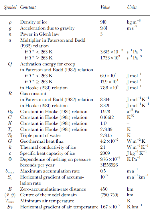
where s is ice-surface elevation, p is ice density and g is acceleration due to gravity. The values used in this study for all constants are given in Table 1. Assuming a non-linear flow law for ice (Reference GlenGlen, 1955), one can find horizontal velocity as

(3)

where h is bedrock elevation, n is usually taken as 3 and the parameter A introduces the temperature dependence of ice viscosity Similar expressions are used to find τ_yz(z) and U_y(z), and vertical velocity, w(z), is found from the horizontalvelocity field using the incompressibility condition. Basal slip is not included in the experiments described here.

Table 1. Constants used in the experiments

The ice accumulation/ablation rate, b, is specified as a radially symmetric function of horizontal position, × and y,

(4)

where b_max is the maximum accumulation rate, S_b the gradient of accumulation-rate change with horizontal distance and E is the distance from the centre of the model domain at which accumulation rate is zero. This parameterization results in a large accumulation area, over most of which accumulation is held constant at 6_max. Around this area, b falls linearly with distance from and rapidly becomes negative (ablation).

The temperature dependence of ice viscosity is incorporated initially using an Arrhenius relation, choosing constants based on work by Reference Paterson and BuddPaterson and Budd (1982)

(5)

where T* (in K) is absolute temperature corrected for the dependence of melting point on pressure, a is a constant of proportionality, Q is the activation energy for ice creep, and R is the universal gas constant. It should be noted that the values of a and Q are different above and below 263 K.

This relationship is replaced in some experiments by that due to Reference HookeHooke (1981)

(6)

In Equations (5) and (6), T* is defined as

(7)

where T_pmp is the pressure-melting-point temperature and T₀ is the triple point of water.

The ice temperature, T, evolves according to

(8)

where U is the horizontal-velocity vector, k is the conductivity of ice and c is its specific-heat capacity. These and the other thermal parameters used in the model are assumed to be independent of ice temperature. Equation (8) forms the second prognostic equation on which the model is based. It contains terms representing vertical diffusion, horizontal advection, vertical advection, and dissipational heat generation, respectively.

Two boundary conditions are required for the integration of Equation (8) forward through time. The upper boundary condition is a specified surface air temperature (T_a)

(9)

where T_min is the minimum surface air temperature and ST the gradient of air-temperature change with horizontal distance. Air temperatures therefore increase in a linear fashion away from the centre of the model domain and are radially symmetric. Several of the experiments reported below employ changes to the value of T_min, which is a control on the overall temperature of the ice sheet and on the presence of patterning.

The boundary condition at the ice-sheet base is

(10)

where G is the geothermal heat flux (assumed constant).

The evolving temperature field is constrained so that it cannot exceed the pressure-melting-point temperature

(11)

An equivalent melt rate is determined where calculated temperatures exceed the pressure-melting point.

The model summarized above is solved using finite differences on a regular horizontal and a stretched vertical grid using mostly implicit methods. A discussion of the numerical methods employed in the model can be found in Reference Hindmarsh and PayneHindmarsh and Payne (1996) and Reference Payne and DongelmansPayne and Dongelmans (1997).

Experiments

The results from a series of experiments designed to address the issues raised in the Introduction will now be discussed. All experiments lasted for 200 kyr by which time a long-term equilibrium had developed. A horizontal grid spacing of 25 km and a time-step of 50 years were employed except in the final set of experiments. Unless otherwise stated, the initial conditions are zero ice on a flat bedrock plane.

The nature of the patterning is such that regions of higher temperatures are always associated with softer ice (increased values of A), faster horizontal velocities and reduced ice thicknesses (Reference PaynePayne and others, in press). In order to simplify the discussion of the results, we will therefore concentrate on the predicted patterns of basal-ice temperature.

The onset of patterning

The onset of patterning was investigated in series of five experiments in which T_min in Equation (9) was given the values 238, 235.5, 233, 228 and 223 K (they will be referred to as experiments A-E). These and all other experiments reported here are summarized in Table 2. The simulated basal-ice temperature field in A is radially symmetric and is dominated by patterning in E (Fig. 1). The extensions of cold, interior ice toward the margin will be referred to as "cold spokes", while "warm spokes" are the intervening divideward extensions of warm, margin ice.

Table 2. Brief summary of the experiments

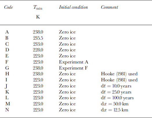
Fig. 1 The predicted pattern of basal temperature (in K) after 200 kyr in experiments with (a) T_min = 238 K (experiment A) and (b) T_min = 223 K (experiment E). The contour interval is 5.0 K and temperatures are not corrected for pressure-melting-point variation. The units of the × and y axes are km.

Much of the information in Figure 1 is redundant. The comparison of a variety of experiments is therefore eased by using simplified representations of this information. This is done in Figure 2 for experiment E. The basal temperature at each model gridpoint is plotted as a function of its distance from the domain centre or ice divide (the black dots in Fig. 2). These temperatures show very little scatter near the divide and towards the margin. This is indicative of radial symmetry. In contrast, points falling 150 to 500 km from the divide show much scatter, which is indicative of pattern formation (see Fig. lb).

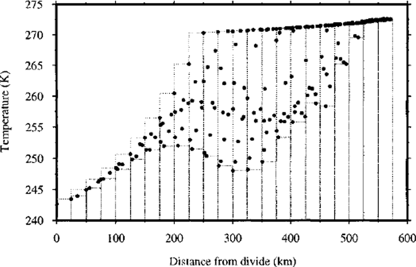
Fig. 2. Basal temperature plotted as a function of distance from the tee divide (at × = 750 km, y = 750 km). The bars indicate the maximum and minimum temperatures within each concentric 25km section of the domain. The difference between maximum and minimum temperature within each section is taken as an index of the strength of patterning

This information can be further summarized by dividing the abscissa into 25 km sections and recording the maximum and minimum within each section (as indicated by the bars in Fig. 2). The difference between the maximum and minimum for each section provides a useful index of the degree of patterning.

The degree of patterning in all five experiments is summarized in Figure 3. The patterning develops between experiments with T_min = 233 K and T_min = 235.5 K. The development of patterning is therefore triggered fairly abruptly over a small temperature range. The contrast between warm and cold spokes increases as T_min decreases. The warm spokes are invariably at pressure-melting point. This difference can therefore be interpreted entirely in terms of cooling within the cold spokes and the majority of this cooling is simply a reflection of the cooler upper boundary condition (T_a).

Fig. 3. The range of predicted basal temperature as a function of distance from the divide for experiments A-E described in the text. The letters refer to the experiment name.

The reversibility of patterning

Two further experiments (each lasting 200 kyr) were undertaken to test whether the patterning shown in Figure 1 is reversible. Experiment F used the final equilibrium state reached by experiment A (which shows no patterning) as an initial condition and imposed a stepped change of T_min from 238 K to 223 K. The results, again in terms of radial temperature anomalies, are shown in Figure 4a. The final equilibrium state of experiment F is directly comparable to that of experiment E (which also employed T_min = 223 K). The relevant lines in Figures 3 and 4a indicate a close but not perfect correspondence. Investigation of the actual basal temperature field indicated that rather than the 12 cold-ice spokes shown in Figure 1b, a total of 20 had formed. The diagonal spokes shown in Figure 1b each split into one central, major spoke and two smaller neighbours.

Fig. 4. The range of predicted basal temperature as a function of distance from the divide for (a) experiments F and (b) experiments G described in the text. The numbers refer to time (in kyr) since the start of each experiment.

Reversibility was tested in experiment G by using the final state produced in experiment Fas an initial condition and reversing the change of T_min back from 223 K to 238 K. The results can be seen in Figure 4b. The patterning rapidly breaks down and radial symmetry is restored after approximately 50 kyr. The final state reached in experiment G is essentially identical to that of experiment A (basal temperature at the divides are within 0.0004 K of each other).

The ice-viscosity relationship used

Experiments H and I are identical to experiments A and E except that the Reference Paterson and BuddPaterson and Budd (1982) (Equation (5)) ice-viscosity relationship is substituted with that of Reference HookeHooke (1981) (Equation (6)). A comparison of the values of A predicted by the two relationships over a temperature range from 223 K to 273 K is shown in Figure 5. The Reference Paterson and BuddPaterson and Budd (1982) relationship predicts higher values of A at temperatures below 250 K and in a narrow range between approximately 268 K and 272 K.

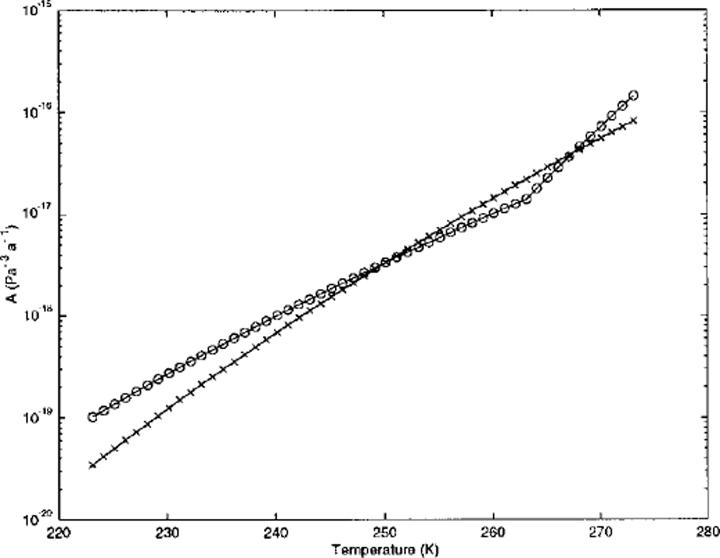
Fig. 5. The values of A predieted by relationships due to Reference Paterson and BuddPaterson and Budd (1982) (circles) and Reference HookeHooke (1981) (crosses) over a temperature range typical of glacier ice. The apparent discontinuity in the Reference HookeHooke (1981) relationship near 273 K is due to the sampling interval used to plot this curve. The relationship is, in fact, continuous throughout.

The basal-temperature distribution at the end of the two experiments is shown in Figure 6, which is directly comparable to Figure 1. The patterning is much stronger in the experiments employing the Reference HookeHooke (1981) relationship. A Tmm of 238.0 K was previously too warm for patterning to develop when employing Reference Paterson and BuddPaterson and Budd (1982), however the patterning is very clearly developed with the Reference HookeHooke (1981) relationship. Patterning in the experiment with T_min = 223.0 K is now so pronounced that the concentration of flow leads to the extension of the ice-sheet margin downstream of warm-ice spokes. This intensification of the patterning is probably because of the step (but continuous) rise in the value of A close to the melting point, which is a feature of the Reference HookeHooke (1981) relationship (Fig. 6).

Fig. 6. The predicted pattern of basal temperature (in K) after 200 kyr in experiments employing the Reference HookeHooke (1981) relationship with (a) T_min = 238 K (experiment H) and (b) T_min = 223 K (experiment I). The contour interval is 5.0 K and temperatures are not corrected for pressure-melting-point variation.

Changing time-step and grid spacing

The time-step (dt) and horizontal grid spacing (da;) used in all of the experiments reported so far are 50 years and 25 km, respectively. It should be noted that the maximum horizontal velocity in these experiments is approximately 80 ma⁻¹, which with dx = 25 km would equate to a maximum time-step (in terms of Courant stability) of 312.5 years. A useful test of the role that numerics plays in the development of patterning is to change the numerical time-step and grid spacing.

A series of three further experiments repeated experiment E with dt = 10, 25 and 100 years (experiments J, K, and L). The results, again presented as radial temperature anomalies, are summarized in Figure 7a. Although the degree of patterning is consistent in all four experiments, there are differences in the geometry of the spoked pattern produced in each experiment. In particular, the pattern produced in experiment J (dt = 10 years) features a total of 20 spokes and was very similar to that described for experiment F above. The results for experiments E and K (dt = 50 and 25 years) were virtually identical.

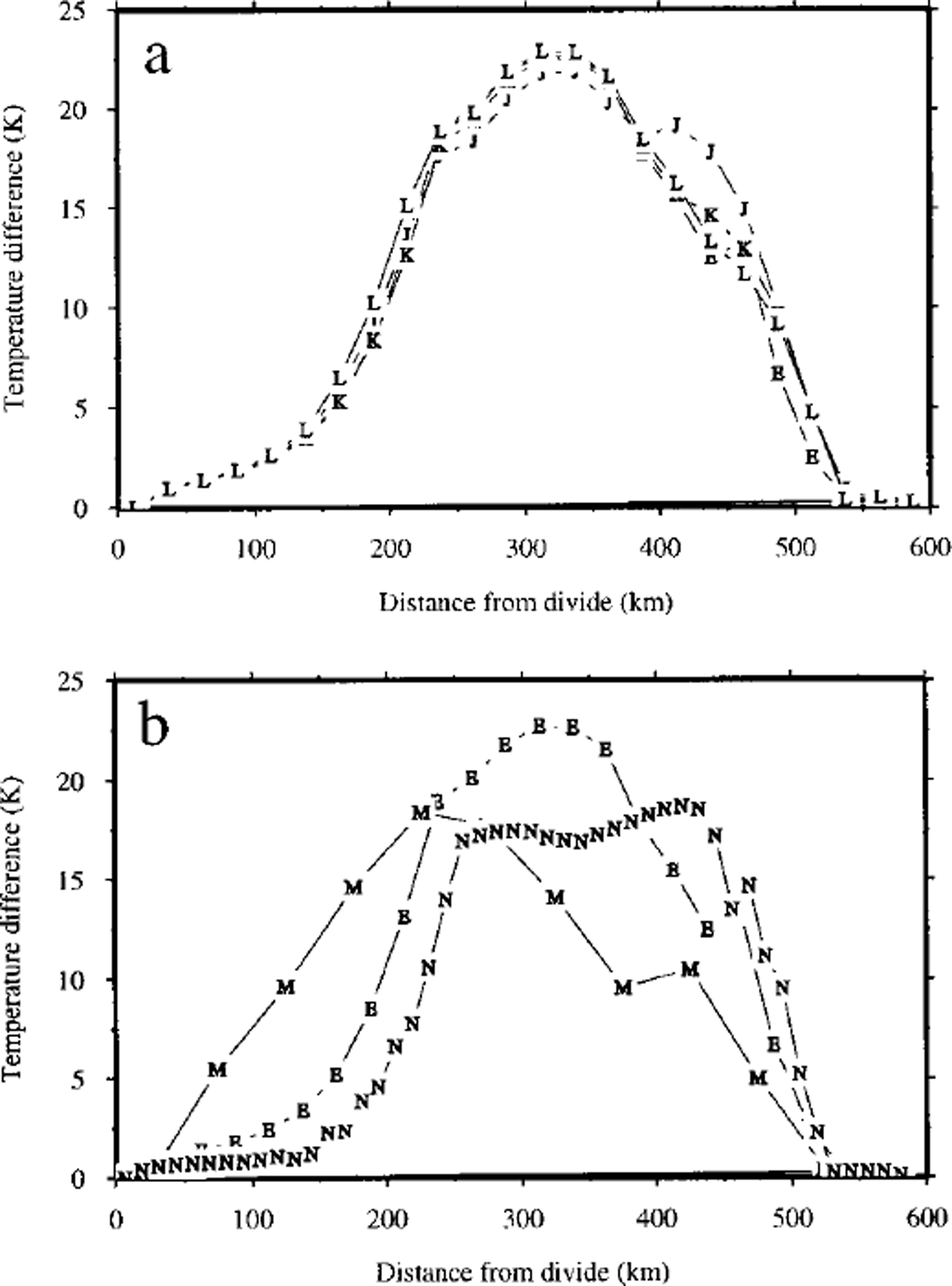
Fig. 7. The range of predicted basal temperature as a function of distance from the divide for (a) experiments with various time-steps (experiments E, J, K and L) and (b) experiments with various horizontal grid spacing (experiments E, M and N). The letters refer to the experiment name.

Experiments with dx = 50 km (M) and dx = 12.5 km (N), in addition to the standard dx = 25 km experiment E are shown in Figure 7b. The radial temperature anomalies reveal very different patterning associated with each horizontal-grid resolution. Inspection of the basal-temperature field produced in each experiment indicates that the number of individual cold-ice spokes rose to 32 in the 12.5 km experiment, while this number fell to 8 in the 50 km experiment (from the 12 of experiment E).

Discussion

The four specific questions raised in the Introduction can now be answered (at least partially).

Patterning develops fairly abruptly between two experiments separated by a 5 K difference in air temperature. Within this 5 K range there is an intermediate form (experiment B) which shows minor undulations in its basal-temperature field. This abrupt onset is thought to be related to the extension of relatively cold ice towards steeper ice-surface slopes near the margin. The mechanism discussed in the Introduction partially relies on the deflection of horizontal ice flow towards warmer, faster-flowing areas of the ice sheet. This type of flow adjustment can occur more easily in areas of steeper surface slope near the margin, rather than in the flatter areas near the ice divide. One of the conditions necessary for pattern formation may therefore be that relatively cold ice (with the potential for warming and hence flow differentiation) occurs in close proximity to relatively steep ice-surface slopes near the margin.

The development of patterning has been shown to be reversible. The details of the final form of patterning do, however, show some dependence on the pathway taken. The number of spokes developed in experiments starting from zero-ice and radial-ice-sheet initial conditions differs. This is an indication that the form of the patterning instability is very sensitive to precise numerical details (as discussed further below).

The discontinuity present in the Reference Paterson and BuddPaterson and Budd (1982) relationship between ice temperature and the value of A is not a necessary condition for pattern development. The relationship derived by Reference HookeHooke (1981) contains no such discontinuity but produces similar behaviour. The exponential nature of these relationships is probably a necessary condition for pattern formation (this could be tested by constructing artificial, linear relationships between temperature and A).

Finally, the details of the patterns developed show dependence on both the numerical time-step and horizontal grid spacing employed. Reference Hindmarsh and PayneHindmarsh and Payne (1996) show that grid-spacing effects predicted ice-sheet geometry because of varying truncation errors. In uncoupled experiments, this affect can amount to as much as 100 m near the margin. These changes in ice-sheet geometry, exaggerated by thermomechanical coupling, may therefore be responsible for the slight differences in the form of the patterning observed here.

It should be stressed that the type of behaviour discussed in this paper is generic to the majority of the large-scale models currently used to simulate the Antarctic and Greenland ice sheets as well as the former, mid-latitude ice sheets. This is clear from the intercomparison reported by Reference PaynePayne and others (in press) and implies that the basal temperatures predicted by these models should be treated with some caution.

There is a strong coincidence between spoke orientation and the underlying finite-difference grid (or diagonals to it) which implies an underlying, numerical control. It is unlikely that this arises simply because we model a circular ice sheet using a rectangular grid. This is because Reference Payne and DongelmansPayne and Dongelmans (1997) found similar behaviour when modelling both square ice sheets and ones whose divide ran parallel to the rectangular finite-difference grid. In addition, ice-sheet models should be able to cope with arbitrary geometries because their main application is to irregular, real-world ice sheets. Future work must address why this grid dependence arises and must seek ways of removing it. One likely area is in the discretization of the dissipation term in the temperature-evolution equation (Equation (8)).

The model discussed in this paper does not incorporate longitudinal stresses. This omission is unlikely to affect the observed patterning because the flow is relatively slow (always ≤ 100 ma⁻¹). The warm-ice spokes are therefore not equivalent to ice streams. Longitudinal stresses may be important at the head of the warm-ice spokes where there are relatively steep horizontal-velocity gradients. However, the incorporation of the dissipation^ heating produced by these longitudinal stresses is likely to exaggerate creep instability and the patterning rather than lessen the effect.