2.1.1. Description of firn

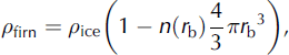
Snow and firn have complex structures of interlocking grains of a variety of shapes and sizes (e.g. Reference LaChapelleLaChapelle, 1992). At low densities (<∼550 kg m⁻³), the firn can be considered a collection of snow grains in a matrix of air (e.g. Reference Wiscombe and WarrenWiscombe and Warren, 1980; Reference Warren, Brandt and GrenfellWarren and others, 2006), while at high densities (>∼800 kg m⁻³) the firn is more like a collection of air bubbles in a matrix of ice (e.g. Reference Mullen and WarrenMullen and Warren, 1988). In between is a transition region, where the difference between grains and bubbles becomes indistinct. The density and specific surface area (SSA), the area of the ice/air interface per unit volume, are two useful parameters for describing the complex structure of firn (e.g. Reference Freitag, Wilhelms and KipfstuhlFreitag and others, 2004). For modeling the optical properties of firn, we follow the widely applied assumption that the scattering and absorption properties of firn can be accurately represented by a collection of spheres with the same SSA and density (e.g. Reference Wiscombe and WarrenWiscombe and Warren, 1980; Reference Dozier, Schneider and McGinnisDozier and others, 1981; Reference Mullen and WarrenMullen and Warren, 1988; Reference Grenfell and WarrenGrenfell and Warren, 1999). The density and SSA uniquely determine an effective grain size and effective bubble size. Note that while the density and SSA are matched, the number of spheres is unlikely to equal either the number of snow grains or bubbles.

Dust, ash, soot and chemical impurities (e.g. sea salt) are also present in firn (e.g. Reference BertlerBertler and others, 2005). The dust and ash particles absorb visible light much more readily than ice and will cause a decrease in returned brightness in the firn (Reference Warren and WiscombeWarren and Wiscombe, 1980; Reference Bay, Price, Clow and GowBay and others, 2001). In typical polar firn, the effects of dust, ash and impurities are small and the optical properties are dominated by scattering of light from ice/air boundaries (e.g. Reference Bramall, Bay, Woschnagg, Rohde and PriceBramall and others, 2005). Large concentrations of soot or other contaminants (e.g. a dense ash layer from a volcanic eruption) could dominate the microstructure-based effects we discuss here, but as these features are rarely found in firn in most parts of Greenland and Antarctica, we do not consider their effect.

2.1.2. Firn reflectance

We investigate the variations in firn reflectance for different combinations of density and either grain or bubble size with a Monte Carlo radiative transfer model. This model is better suited to our purposes than the adding-doubling (e.g. Reference HansenHansen, 1971) and multi-stream methods (e.g. Reference BohrenBohren, 1987) used in other studies of ice surface albedo, because it allows treatment of a curved boundary and a point-like light source. The model determines the wall reflectance as a function of grain size, density and borehole radius. This model was adapted from a simple Monte Carlo code designed for analysis of radiation propagation in human tissue (Reference PrahlPrahl, 1988); the code will be available at: http://gcmd.nasa.gov/getdif.htm?waddington_0335330.

Our model tracks packets of photons that enter optically thick firn at a single location, simulating a collimated-beam light source. We assume no Fresnel reflection on the borehole wall. At each scattering event, a new direction for the packet is chosen from a Henyey–Greenstein (H-G) phase function (Reference Henyey and GreensteinHenyey and Greenstein, 1941). The H-G phase function requires specification of the asymmetry parameter, g, the mean cosine of the phase angle of scattered photons. After several scattering events, the H-G phase function accurately approximates true phase functions with the same asymmetry parameter and allows high computational efficiency compared to calculations that use more detailed approximations of the phase function (e.g. Reference PettyPetty, 2006). A value of g = 0 yields isotropic scattering, while g = 1 yields pure forward scattering. Snow grains that are large compared to the wavelength of light are strongly forward-scattering, with g equal to ∼0.89 (Reference Wiscombe and WarrenWiscombe and Warren, 1980); spherical air bubbles have g values between 0.85 and 0.86 (Reference Mullen and WarrenMullen and Warren, 1988).

At the exit location, the contribution of each packet to the exit intensity is determined using an attenuation factor chosen depending on whether the modeled firn is most similar to a collection of ice grains in air or to a collection of air bubbles in ice:

(1)

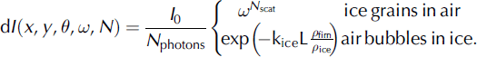
Here x and y are Cartesian coordinates on the surface of the slab of firn, θ is the angle at which the light exits the surface relative to the vertical axis, z, I ₀ is the initial intensity and N _photons is the number of packets tracked. For ice grains in air, the absorption is determined by ω, the single-scatter albedo for ice grains, and the number of scattering events, N _scat. For air bubbles in ice, the single-scattering albedo of the air bubbles is treated as unity, and the factor

accounts for absorption as a photon travels through the ice. Here k _ice is the absorption coefficient for ice (Reference Warren and BrandtWarren and Brandt, 2008), ρ _firn and ρ _ice are the densities of the firn and ice, and L is the distance the photon traveled. The total absorption is assumed to be proportional to the volumetric ice concentration (Reference Mullen and WarrenMullen and Warren, 1988). This process is repeated for ∼10⁷ photons.

The outgoing intensity is in units of energy steradian⁻¹ L _scat ⁻². The scattering length, L _scat, is the e-folding distance for extinction of a photon along a particular direction by scattering, and is found by

(2)

where σ _scat is the scattering coefficient, n(r) is the density of scatterers per unit volume, r is the mean radius of the scattering particle and Q _scat is the scattering efficiency. The scattering efficiency gives the total scattering cross section for the particle per unit cross-sectional area; it depends on the wavelength of the radiation and the size and material properties of the particle. It is usually ∼2 because the path of a photon traveling near a snow grain or bubble can be deflected by diffraction.

The density of scatterers, n(r), can be equated to mass density of the firn for grains in air,

(3)

where r _g is the radius of the ice grains. For bubbles in ice,

(4)

where r _b is the radius of the bubbles. An equation for the scattering length as a function of grain size and density results from combining Equations (2) and (3) for grains in air:

(5)

Combining Equations (2) and (4) for bubbles in ice,

(6)

The model was designed to use units of the number of scattering lengths, so that the results from a single run can produce reflectances for different combinations of grain or bubble size and density. The only parameter of the firn that is specified in the Monte Carlo code is g. The output can be scaled to length units for any combination of grain or bubble size, density and scattering efficiency (appropriate values discussed below).

2.1.3. Applicability to wide density range

In our modeling results, we use parameters appropriate to scattering of light by large particles. The scattering efficiency is ∼2 for both ice grains in air (e.g. Reference Warren, Brandt and GrenfellWarren and others, 2006) and air bubbles in ice (Reference Fu and SunFu and Sun, 2001). The single-scatter albedo for ice grains was calculated using

(7)

following Reference Warren, Brandt and GrenfellWarren and others (2006). For air bubbles in ice, we assume there is no significant absorption during the scattering events (ω = 1) and account for absorption with the ice-path length factor in Equation (1). At transition densities, neither approximation is clearly more accurate than the other. For the large ice grains considered here, combining Equations (1), (5) and (7) gives the average absorption per scattering event as approximately 1.28k _ice ρ _firn /ρ _ice. By contrast, Equation (1) for bubbles in ice gives the average absorption per scattering event as ∼k _ice ρ _firn /ρ _ice, or about 30% less. The difference arises primarily because during a scattering event from an ice grain in air, photons take a complicated path that reflects multiple times off the air–ice interface, increasing the path length in the ice grain. Over the course of a particle’s path through the firn, the larger asymmetry parameter for ice grains also tends to lead to greater path lengths than those calculated for bubbles, leading again to more absorption.

The grains-in-air approximation has been validated against field measurements (e.g. Reference Hudson, Warren, Brandt, Grenfell and SixHudson and others, 2006) for densities smaller than the close-packed density. Theoretical arguments suggest this formulation should give reasonably accurate results for close-packed grains (Reference Wiscombe and WarrenWiscombe and Warren, 1980). The bubbles-in-ice approximation matches measured reflectances for ρ _firn > 800 kg m⁻³ (Reference Mullen and WarrenMullen and Warren, 1988), but has not been tested at lower densities. We could transition smoothly between the two approximations by weighting each according to the density in the transition region. However, such an approach has two main problems: (1) we are aware of no measurements that indicate how the transition between the two approximations occurs, and (2) creating a smooth transition does not add insight into the processes causing variations in BOS brightness measurements. In the remainder of the paper, we show results from the grains-in-air approximation for all densities, and we present the results of the bubbles-in-ice approximation for ρ _firn> 550 kg m⁻³ for comparison. Hereafter, we discuss the variations in firn microstructure in terms of density and grain size rather than bubble size.

2.1.4. Tracking the return of photons to boreholes

The cylindrical geometry of the borehole reduces the effective albedo of the wall; as the borehole radius decreases, photons become less likely to re-encounter the borehole during their random walk through the firn. To derive reflectances for a curved borehole wall, the Monte Carlo process is modified to give reflectances as a function of a scaled borehole radius, Γ, equal to the borehole radius divided by L _scat. In this model, the borehole axis runs parallel to the z-axis. The photons enter the borehole wall (at the origin of the coordinate system), traveling in the −x direction, and re-enter the borehole when (x−Γ)² + y² <Γ². The same photon may be tracked from a single starting position through several boreholes of different radius as long as the position, angle, distance traveled and number of scattering events is recorded the first time each photon reenters a borehole of given diameter. The calculation is terminated when the photon re-enters the borehole with the smallest Γ, corresponding to the largest scattering length.

2.2.1. Persistence of Vision ray-tracing algorithm

We use a ray-tracing algorithm to investigate how multiple reflections within the borehole produce variations in measured brightness. The ray-tracing package is the Persistence of Vision Raytracer (POV-Ray, http://www.povray.org). This has been used in a variety of research projects, including modeling radiant fluxes between building surfaces in urban environments (Reference LagouardeLagouarde and others, 2010) and modeling light reflections in forest canopies (Reference Casa and JonesCasa and Jones, 2005). It tracks light rays from a source, through multiple reflections from objects with specified reflective properties, back to a camera. The light reaching the camera is calculated as a function of angle to produce an image. The modeled camera and light source were based on the GeoVision Jr^TM borehole video camera used by Reference Hawley, Waddington, Alley and TaylorHawley and others (2003). The light source is a set of eight white light-emitting diodes (LEDs) forming a ring of 1.6 cm radius around the camera and angled out from the camera’s optical axis by ∼20°. We verified that the ray tracing reproduced the proper light emission, by simulating the illumination pattern of the model camera onto a diffuse, white surface and comparing the resulting images with the illumination pattern of the GeoVision Jr ^TM on a sheet of white paper. The borehole was modeled as a 10 cm diameter open cylinder, with the camera and light source at the center looking down the cylinder.

POV-Ray allows the user to specify both the fraction of light reflected and how that light is reflected from an object. Our choices for the fraction of light reflected from the borehole wall were guided by the radiative transfer results discussed below. We used a Lambertian reflectance model to describe the bidirectional reflectance function of the borehole wall. A Lambertian surface scatters light such that an observer perceives the same brightness from any viewing angle, and approximates our modeled surface well (see section 3.1.2). To model Lambertian reflectance, POV-Ray uses the Radiosity algorithm (Reference Goral, Torrance, Greenberg and BattaileGoral and others, 1984), in which surfaces are discretized into facets with Lambertian reflectance and the radiative transfer equation is solved to determine the radiant flux from each facet to each other facet.

3.1.1. Borehole wall reflectance

Borehole wall reflectances are plotted as a function of grain size or bubble size for a series of borehole sizes in Figure 1a for three firn densities. The calculations were performed with an absorption coefficient of 0.12 m⁻¹,appropriate for light of 600 nm wavelength (Reference Warren and BrandtWarren and Brandt, 2008). Decreasing the borehole radius decreases the reflectance because fewer photons find their way back into the borehole. This effect is shown schematically for ice grains in Figure 2a. The borehole reflectance is significantly greater for the bubbles-in-ice than the grains-in-air approximation. As discussed above, this is caused both by the lesser absorption per scattering event and by the shorter path lengths that result from the lower asymmetry parameter for bubbles, g = 0.85, versus grains, g = 0.89. The pattern of reflectance variation with borehole size is similar for the two approximations, but the difference in magnitude between the two is greater than that caused by a shift in density of 200 kg m⁻³. This suggests that the grain shape plays an important role in the brightness variations, which we have not modeled.

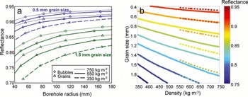
Fig. 1. The borehole wall reflectance depends on the grain size, density and borehole diameter. (a) Reflectance as a function of borehole radius for three different densities. For the two larger densities, the reflectance is calculated with the grains-in-air approximation (triangles) and the bubbles-in-ice approximation (circles). Grain sizes shown are 0.5 mm (blue) and 1.5 mm (green). (b) Reflectance for a 100 mm diameter borehole. The grains-in-air approximation is solid; bubbles-in-ice approximation is dashed. In both (a) and (b), the bubble size varies but matches the SSA and scattering length of the grain size and density combination.

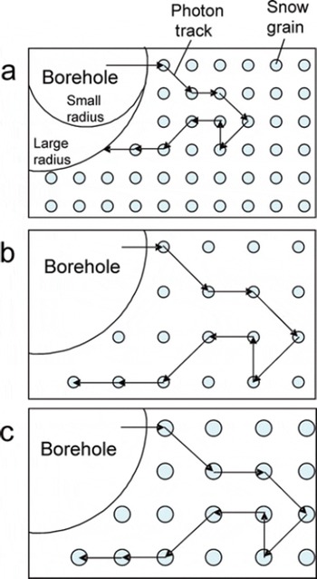
Fig. 2. Schematic showing the effects of varying the borehole radius (a), density (b) and grain size (c) on the likelihood of a photon returning to the borehole. Light-blue filled circles are snow grains. Arrows show photon paths. The photon scatters in the same direction at corresponding scattering events in each scenario. In (b) and (c) the photon does not return to the borehole because the scattering length has increased.

In Figure 1b, the reflectance is also seen to depend on the density and the grain size, both of which determine the scattering length of the firn; fewer photons will return to the borehole for firn with a greater scattering length. Figure 2 shows how a photon that scatters in the same direction at each scattering event may not return to the borehole because of either an increase in grain size or a decrease in density. The decrease in reflectance from a decrease in density is due entirely to the change in scattering length, but an increase in grain size has a dual effect: a larger grain size both increases the scattering length and decreases the single-scatter albedo. Though variations in grain size change the borehole wall reflectance more than do variations in density, variations in either parameter can cause reflectance variations of the magnitude observed with BOS.

3.1.2. Distribution of light returned to the borehole

The radiative transfer model also determines the spatial displacement between the location at which photons enter the borehole wall in a single collimated beam and the location where they return. For high scattering lengths and/ or high single-scatter albedos, the displacement can complicate small-field-of-view measurements of firn albedo and blur reflected-light imagery within boreholes. A simple way to describe the extent of spreading is the mean radius of returned energy,

(8)

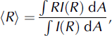
where R is the distance between the point where the photon enters and exits the firn. The mean radius of returned energy depends upon the grain size, density and asymmetry parameter. Figure 3a shows the displacement for different densities and grain sizes and an asymmetry parameter of 0.89. The returned energy in each increment of radius [R, R+dR] and the intensity for each increment of radius are shown as a function of radius (Fig. 3b). The intensity falls off more quickly than the returned energy because the area increases with increasing radius. The returned energy is greater at 5 mm than at smaller radii because the fractional area that a photon can return to increases rapidly at small radii and has a greater effect than the fall-off in returned photons with radius.

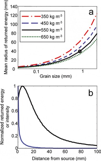
Fig. 3. (a) For a flat surface, the mean radius of returned energy can be calculated as the radius of the circle inside which half the energy exits the firn. It is defined in Equation (7). The circle marks the properties used in (b). (b) The fall-off of returned energy (black) and intensity (blue) with distance from the source for a flat wall and firn with a 1 mm scattering length. The returned energy is greater at 5 mm than at smaller radii because the percentage increase in area to which a photon returns increases faster than the fall-off in returned photons.

The intensity of the photons leaving the borehole wall as a function of angle relative to the wall normal, θ, is shown in Figure 4. The normalized intensity curve matches the normalized curve for a Lambertian surface, for which I(θ) = I(θ) cos(θ). The agreement is typically within a few percent, with a maximum difference of 15% at exit angles of ∼75°. The close agreement shows that it is appropriate to represent the borehole wall in the ray-tracing model as a Lambertian surface.

Fig. 4. Comparison of the intensity by exit angle for the radiative transfer model (blue with crosses) and the expected intensity for a Lambertian surface (red). A Lambertian surface has the same brightness from all viewing angles described by I(θ) = I(θ) cos(θ), where I is intensity and θ is the exit angle.

3.2.1. Simulations

We conducted two types of simulations: variations in the borehole wall and variations in the camera position or orientation. For variations in the borehole wall, we added a feature to the borehole: either a dark band for a change in firn properties, or an imperfection, a ridge or gouge, as might be produced during drilling. For each feature type, we simulated a BOS log by generating a series of frames in which the camera position varied from 1 m above to 1 m below the feature.

We reduced each of these frames to a single brightness value following the technique of Reference Hawley, Waddington, Alley and TaylorHawley and others (2003), averaging the pixels in a narrow annulus around the borehole for each frame to give the brightness for ∼1 vertical cm of the borehole wall. The annulus is located 10 cm below the camera (Fig. 5). All brightness logs are presented as the percentage change from the brightness in a borehole with the same wall reflectance but no feature. The y-axis has been re-centered such that 0 indicates when the center of the annulus is located on the center of a feature (Fig. 5b). This permits the change in recorded brightness with distance from the feature to be easily seen.

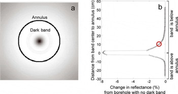
Fig. 5. (a) A borehole video frame created with the Persistence of Vision ray-tracing program. The annulus marks the pixels whose brightness values are averaged to create one brightness measurement. A band of lower reflectance is shown below the annulus. Wall reflectance is 80%, band reflectance is 5.26% less. (b) The percentage difference in brightness compared to a borehole with no dark band. Lowering the camera down a borehole is simulated by making a series of images (like (a)) as the feature is moved up the borehole relative to the camera. The red circle shows the brightness value from the image in (a).

We also produced series of images that simulate the variations in the camera orientation and position that will occur if the stabilizers for the camera lose contact with the borehole wall. The camera can either point away from the borehole axis or move from the center of the borehole. In the first series of images, we varied the pointing angle of the camera from 0 to 2.5° from the borehole axis. In the second series of images, we moved the camera from the center of the borehole to 3 cm off-center. In both series, the borehole wall had a consistent reflectance for the entire depth.

3.2.2. Accounting for the spreading of light in firn

In the ray-tracing algorithm, the light rays reflect off the borehole wall at the location of impact; they do not spread through the firn. Even though some features (e.g. the ridges and gouges) are likely covered in drill dust (small snow grains produced by drilling) that makes the scattering length lower than that of the surrounding firn, the spreading of light will still be significant (Fig. 3a). To approximate the spreading of light, we convolved the brightness logs for the dark-band and ridge-and-gouge simulations with a 5 cm wide kernel based on the pattern of intensity found with the radiative transfer model for firn with a 1 mm scattering length (Fig. 3b). We performed a second convolution with a 5 cm Gaussian kernel to approximate the filtering done in post-processing (e.g. Reference Hawley, Waddington, Alley and TaylorHawley and others, 2003).

3.2.3. Band of lower reflectance

A layer in the firn with a different density and/or grain size than the local background norm was represented by a band of different reflectance. Dark bands of 5.26% less reflectance than the wall reflectance were modeled. The 5.26% drop maintained consistency with the 95% background-reflectance case when the dark band was 90% reflective (5.26% is 0.05/0.95). The magnitude of the reflectance drop was based on reflectance changes of 1.5% and 3%, which we calculated from measurements of porosity and SSA for firn of depths 15 and 51 m from North Greenland (Reference Freitag, Wilhelms and KipfstuhlFreitag and others, 2004). The larger 5.26% drop helps reduce the numerical noise in the ray-tracing calculations. Simulations were run for three layer thicknesses, 2, 5 and 10 cm, and for two background borehole wall reflectances, 80% and 95%. The 95% simulations most closely resemble upper firn conditions of small grains and low scattering lengths. The 80% simulations are similar to deeper firn conditions, with larger grains and longer scattering lengths.

In all simulations, the drop in brightness measured at the band was greater than the 5.26% drop in reflectance of the band. Figure 6a shows the brightness variations for the three different bandwidths at 80% and 95% reflectance. The greater the borehole wall reflectance, the greater the fractional change in brightness at the center of the band. Futhermore, the decrease in brightness increased with the thickness of the band. The dark band also reduced the brightness beyond its edges: areas adjacent to the band, but above or below it, appeared darker, an effect that is more pronounced down-borehole from the dark band. The darkening occurs because the dark band absorbs some of the energy that is multiply reflected around the borehole. Having the dark band near the light source decreases the energy available to illuminate the borehole wall, and the brightness recorded at the annulus decreases, even if the annulus is not on the dark band.

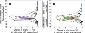
Fig. 6. Percentage decrease in brightness due to borehole-wall multiple reflection effects. Dark bands have widths of 10 cm (dashed), 5 cm (dotted) and 2 cm (solid) and 5.26% lower reflectance than the borehole wall. Horizontal lines indicate one borehole radius (5 cm) away from the edge of a dark band. (a) 80% (green) and 95% (purple) wall reflectance. (b) 80% wall reflectance in green is same as in (a). To approximate the spreading of light in firn, we convolve the brightness log with a 5 cm kernel based on the intensity fall-off from the radiative transfer modeling (red). To simulate post-processing smoothing, we convolve the brightness log with a 5 cm Gaussian kernel (light blue).

The effects of light spreading through the firn and post-processing smoothing are shown in Figure 6b. The spreading of light decreases the magnitude of the brightness drop and smooths the measured signal at the band edge. The brightness change is reduced more for the thinner bands. The Gaussian smoothing has a similar effect, though the magnitude of the brightness drop at the center of the dark band is reduced more, particularly for the 2 cm thick bands.

3.2.4. Ridges and gouges

Imperfections in the borehole wall are often formed when the drill is stopped to extend the drill stem length or to recover a core section. To simulate these imperfections, we generated a set of images, where either a ridge or a gouge was added to the borehole circumference (Fig. 7a and b). In a cross section along the length of the borehole, the ridge is a semicircular projection of radius 1 mm into the borehole; the gouge is a depression. The brightness log for a borehole with a ridge at 80% wall reflectance is shown in Figure 7c. The ridge causes a ring of high brightness and a smaller shadowed area below. The brightness is affected more below the ridge than above it; no effect of the ridge is noticeable one borehole radius (5 cm) away from the ridge in either direction. Simulations with a wall reflectance of 95% were similar, though the magnitude of the brightness variation was less because of the large amount of light already reaching the camera.

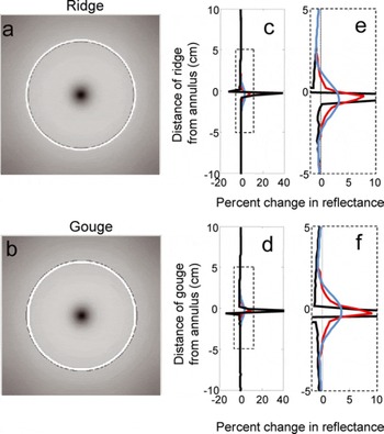
Fig. 7. Wall reflectance is 80%. (a) Ray-tracing image of borehole with a 1 mm ridge 10 cm below camera. Annulus is not shown. (b) Image of borehole with a 1 mm gouge 10 cm below camera. (c–f) Thick black curves show brightness change as camera is lowered past feature. The large (∼40%) reflectance changes using ray tracing only are unrealistic because spreading of light in firn is not incorporated in the ray-tracing model. To approximate the spreading of light, we convolve the brightness log with a 5 cm kernel based on the intensity fall-off from the radiative transfer modeling (red). To simulate post-processing smoothing, we convolve the brightness log with a 5 cm Gaussian kernel (light blue). Dashed boxes in (c) and (d) show area enlarged in (e) and (f).

The simulation of a BOS measurement with a 1 mm gouge is shown in Figure 7d. As in the ridge case, both a ring of high brightness and a smaller shadowed area are created, but in this case the shadowed area is higher in the borehole. The brightness increase when the annulus is centered on the gouge is similar to that of the ridge. The brightness immediately above and below the gouge is decreased, but no effect is noticeable at distances of one borehole radius away.

The effect of light spreading in the firn and of smoothing in post-processing on these logs is shown in Figure 7e and f. The brightness peak of the ridge or gouge is substantially muted, but the brightness increase is spread over a larger vertical distance. The sharp drop in brightness is no longer observed. The brightness record becomes more similar to the brightness variations caused by variations in firn properties (Fig. 6b). Convolving the brightness logs with the Gaussian kernel has a similar effect. The magnitude of the brightness signal is reduced but at the expense of making the signal from the wall imperfections visually more similar to a signal that might result from annual-scale layering.

3.2.5. Camera position and orientation

The effects of the camera pointing off the borehole axis and the camera pointing straight down but being offset from the center of the borehole are shown in Figures 8 and 9. The brightness was calculated in two ways: (1) uncorrected – where, as above, the brightness was the average over an annulus of pixels 10 cm below the camera, centered on the middle of the image; and (2) corrected – where the annulus is re-centered on the darkest pixel in the image, which is a best guess of the bottom of the borehole. The brightness was also calculated for a half-annulus on each side of the borehole. The camera points (or is offset) toward the + side, and points (or is offset) away from the – side. For all images, the borehole wall reflectance was 80%.

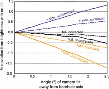
Fig. 8. Reflectance difference for the camera pointing off the borehole axis. Wall reflectance is 80%. Full annulus (black). The camera is pointing toward the + side (blue) and away from the − side (orange). Solid curves have no correction to the processing. Dashed curves improve the processing by re-centering on the darkest point in the image which is interpreted as the borehole center.

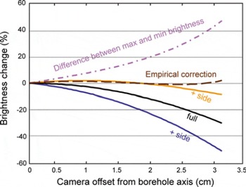
Fig. 9. Brightness change between a camera offset in the borehole and one centered. The camera is offset toward the + side (blue) and away from the − side (orange). The empirical correction (brown dashed) uses the full annulus brightness and the difference between the maximum and minimum brightness (purple dash dot) of the annulus to find the best estimate of what the brightness would be if the camera were centered in the borehole. See text and Equations (9) and (10) for description of empirical correction.

As the camera tilt increases to 2.5°, the uncorrected half-annulus averages vary relative to the untilted image by up to 1.5% (Fig. 8). Correcting the averaging process by re-centering the annulus reduced this effect by about half. The uncorrected brightness variations of the two sides partly cancel each other for the full-annulus averages, but variations up to 0.5% can persist. Re-centering the annulus on the bottom of the borehole reduced the brightness variations to <0.2%. Simulations with boreholes of 20% and 98% wall reflectance showed similar improvements.

The effect of the camera being offset from the center of the borehole is shown in Figure 9. The variations in brightness are significantly larger than in the tilted-camera case, with a drop in brightness for an offset of 3 cm as large as 35% for the whole annulus, and as large as 55% for the + side. Re-centering the annulus does little to reduce the change in brightness because the center of the borehole does not move significantly due to the camera displacement. A different correction is required for these errors. The smooth shape of the brightness-change vs offset curve allows us to calculate a correction as a function of two values that can be determined for any annulus on any video frame: the mean brightness for the annulus, B ₀, and the difference between the maximum and minimum brightness on the annulus, δB. The corrected brightness, , can be found by

(9)

If the correction were perfect, the corrected brightness would equal the brightness of the same annulus when the camera is centered in the borehole. We used a second-degree polynomial for f,

(10)

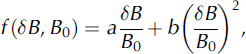
and found the values for a and b that minimized the misfit between and the zero-offset brightness. A third-degree polynomial did not produce a noticeably better correction. For 80% wall reflectance and offsets less than 3 cm, the optimal coefficients were a = 0.51, b = 0.3. This corrected the brightness to within 2.5% of the centered camera case. These same coefficients produced similar improvements for a wall reflectance of 98%. For a wall reflectance of 20%, the corrected brightness still varied from the camera-centered brightness by ∼6%.