


1. INTRODUCTION
The Himalayan region has one of the largest concentrations of glaciers outside of the polar regions with a glacier coverage (including the Karakoram) of ~40 800 km2 (Bolch and others, Reference Bolch2012). Himalayan glaciers are of interest for several reasons. Water discharge from Himalayan glaciers contributes to the overall Himalayan river runoff (Immerzeel and others, Reference Immerzeel, van Beek and Bierkens2010) and the precipitation, along with snow and ice melt, also affect the runoff considerably (Bhambri and others, Reference Bhambri, Bolch, Chaujar and Kulshreshta2011a). Singh and others (Reference Singh, Haritashya and Kumar2008) and Bhambri and others (Reference Bhambri, Bolch, Chaujar and Kulshreshta2011a) reported that on an average, yearly snow and glacier melt contributed ~97% of water, measured at Bhojbasa (~4 km downstream from Gangotri Glacier snout and ~3780 m a.s.l.) to the Ganga Basin near the terminus of Gangotri Glacier. Although far from the terminus of Gangotri Glacier (Kaser and others, Reference Kaser, Großhauser and Marzeion2010), this percentage decreases. In addition water discharge from Himalayan glaciers is also important for irrigation and hydropower generation (Singh and others, Reference Singh, Polglase, Wilson, Jain, Singh, Kumar, Kumar, Singh and Sharma2009). Gangotri Glacier is the largest glacier in terms of length (~30 km) and area (~144 km2) in the Garhwal Himalayas (Srivastava, Reference Srivastava2012). The Bhagirathi River originates from the snout (Gaumukh ~3950 m a.s.l.) of Gangotri Glacier, which is the main source of the River Ganges. The glacier originates from the Chaukhamba group of peaks (~6853–7138 m a.s.l.) and flows northwest towards Gaumukh (Bhambri and others, Reference Bhambri, Bolch and Chaujar2012). Gangotri Glacier is one of the most sacred shrines in India, with immense religious significance. Being the main source of the River Ganges, the most sacred river to the Hindus, it attracts thousands of pilgrims every year.
High resolution multitemporal and multispectral satellite data have abundant potential to study the glaciers in terms of extent, surface properties, surface velocity and temporal mass balance (Bolch and others, Reference Bolch2010). Declassified imagery such as Corona and Hexagon has proven to be especially useful data source for mapping historic extents of glaciers and generation of digital terrain model (DTM) for mass-balance studies (Surazakov and Aizen, Reference Surazakov and Aizen2010; Pieczonka and others, Reference Pieczonka, Bolch and Buchroithner2011; Holzer and others, Reference Holzer2015; Pellicciotti and others, Reference Pellicciotti2015). These declassified imageries can also be used for comparisons with glacier outlines derived from topographic maps (Bhambri and Bolch, Reference Bhambri and Bolch2009).
Various methods have been applied for the on-going mapping and monitoring of the Gangotri Glacier, which have resulted in considerable differences in glacier retreat rates (e.g. Srivastava, Reference Srivastava, Srivastava, Gupta and Mukerji2004; Kumar and others, Reference Kumar, Dumka, Miral, Satyal and Pant2008; Bhambri and Chaujar, Reference Bhambri and Chaujar2009; Bhambri and others, Reference Bhambri, Bolch and Chaujar2012). The snout position of Gangotri Glacier was mapped first by Auden, (Reference Auden1937) in 1935 using a plane table survey at a scale of 1:4800. It was postulated from various geomorphological features that the glacier retreated at a rate of 7.35 m a−1 from 1842 to 1935. Subsequent surveys were conducted by the Geological Survey of India (GSI) to measure the retreat rate of the Gangotri Glacier snout. Inherent inconsistency and uncertainty in different methods are however still major issues. Therefore, regular consistent monitoring is important for improving our knowledge of glacier response to climate change. In-situ measurements of glacier mass balance or glacier velocity for a large debris-covered glacier, such as Gangotri Glacier, are logically difficult and hence hardly feasible due to its size and characteristics. In contrast to glacier mass balance, glacier length change shows only the indirect and delayed response of the glacier to climate change. Given that the response time of large debris-covered Gangotri Glacier is likely much longer than that of smaller glaciers in the Garhwal region (Thayyen, Reference Thayyen2008), the determination of glacier mass balance is needed for precise knowledge of the glacier health. Moreover, to understand the glacier response to climate change, investigations of the seasonal behaviour of glacier surface dynamics are also indispensable. To our knowledge there are no published studies addressing both the temporal mass balance and seasonal variation of glacier surface velocity for this large debris-covered glacier. Thus, the main goals of the present study are (1) determine length and area variation at the snout of the Gangotri and its tributary glaciers from 1965 to 2015 using declassified imageries (KH-4A Corona, KH-9 Hexagon), imageries from Landsat Mission and Advanced Spaceborne Thermal Emission and Reflection Radiometer (ASTER) imageries (2) to assess the geodetic glacier mass budget for the last five decades using DTMs from declassified imageries (KH-4A Corona) and ASTER imageries; and (3) to study the seasonal ice surface velocity for the last two decades.
2. DESCRIPTION OF THE STUDY AREA
Gangotri Glacier is located in Garhwal Himal in Western Himalaya (Fig. 1). It belongs to the Uttarkashi district of the federal state of Uttarakhand in India. The glacier comprises four main tributaries: two tributaries, Kirti Bamak and Ghanohim Bamak, flow from the left and other two tributaries, Swachhand Bamak and Maiandi Bamak, flow from the right with respect to the main glacier flow (Srivastava, Reference Srivastava2012). There are three other tributary glaciers, viz. Meru Glacier (length ~7.55 km) on left side and Chaturangi Glacier (length ~22.45 km) and Raktavarn Glacier (length ~15.90 km) on right side (Srivastava, Reference Srivastava2012), which have been connected with the Gangotri Glacier in the past. Bhambri and others (Reference Bhambri, Bolch, Chaujar and Kulshreshta2011a) estimated that the Gangotri and its tributary glaciers cover a total area of ~210.60 km2, ~29% of which is covered by debris. The average width of the glacier is 1.5 km (Srivastava, Reference Srivastava2012) and the estimated glacier volume vary between ~20 and ~30 km3 (Frey and others, Reference Frey2014). It covers an elevation range of ~4000 to ~7138 m a.s.l. (Srivastava, Reference Srivastava2012).
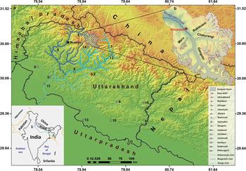
Fig. 1. Location of the study area in Himalaya (a) Bhagirathi Basin with Alaknanda, Bhagirathi and Ganga River System (b) Gangotri and its tributary glaciers. International boundaries are tentative only.
Thayyen and Gergan, (Reference Thayyen and Gergan2010) reported that the Garhwal Himalayan glaciers are usually fed by summer monsoon and winter snow fall. According to the recent study by Maussion and others (Reference Maussion2014), the glaciers in Garhwal Himalaya are fed mainly by winter accumulation. The maximum snowfall due to western disturbances usually occurs from December to March as mentioned by Dobhal and others (Reference Dobhal, Gergan and Thayyen2008). Mean annual air temperature and annual precipitation during 1971–2000 at Mukhim station, (~1900 m a.s.l.; ~70 km from the snout of Gangotri Glacier) shown in Figure 1, were found to be 15.4°C and 1648 mm respectively by Bhambri and others (Reference Bhambri, Bolch, Chaujar and Kulshreshta2011a) using the data recorded by Indian Meteorological Department (IMD) and Snow and Avalanche Study Establishment (SASE). The meteorological observatory at Bhojbasa (~3780 m a.s.l.), which is ~4 km from the snout of Gangotri Glacier (Fig. 1), recorded 11°C, –2.3°C and ~546 mm average annual maximum, minimum temperatures and average winter snowfall respectively as reported by Bhambri and others (Reference Bhambri, Bolch, Chaujar and Kulshreshta2011a). Precipitation data from this also indicated on an average Gangotri and the surrounding areas receives >15 mm of daily rainfall during the summer season (Singh and others, Reference Singh, Haritashya, Ramasastri and Kumar2005).
3. REVIEW OF CURRENT KNOWLEDGE
Gangotri Glacier is one of the best documented glaciers in the Indian Himalaya with regards to the monitoring of its snout position. It has been long observed in different studies that the glacier has been retreating continuously since 1935 (Auden, Reference Auden1937). Based on the estimates reported in articles (Tangari and others, Reference Tangari, Chandra, Yadav, Srivastava, Gupta and Mukerji2004; Bhambri and Chaujar, Reference Bhambri and Chaujar2009; Bahuguna and others, Reference Bahuguna2007), it can be stated that Gangotri glacier retreated at a higher rate from ~1970–2000. The rate of retreat was less both before ~1970 and after ~2000 (Jangpangi, Reference Jangpangi1958; Vohra, Reference Vohra, Lall and Moddie1981; Bhambri and others, Reference Bhambri, Bolch and Chaujar2012; Srivastava, Reference Srivastava2012). For more details of the published results about the terminus retreat of Gangotri Glacier see Figure 2 and Table 1 in the Supplement.
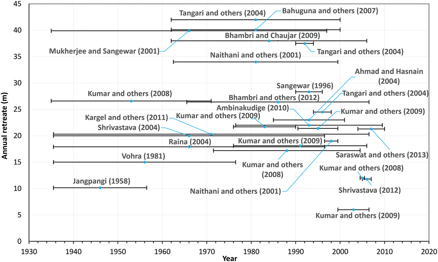
Fig. 2. The annual retreat estimates of the Gangotri Glacier terminus as calculated by various authors. The horizontal bars correspond to the observation period. The mid-point of each bar is marked by a blue point. An artificial shift of 0.1 m was introduced for several bars to improve the legibility. The spread of the retreat values illustrates a large uncertainty of the estimates. For more details see the Table 1 in the Supplements.
The areal extent of the Gangotri Glacier has been studied from 1962 by Negi and others (Reference Negi, Thakur, Ganju and Snehmani2012), and a 6% glacier area loss between 1962 and 2006 was found using SOI map and Cartosat-1 data. A considerable reduction in glacier area was also reported during the period from 1965 to 2006 (Kumar and others, Reference Kumar, Areendran and Rao2009, Bhambri and others, Reference Bhambri, Bolch and Chaujar2012). A 1962 SOI map has been used as a baseline for a number of studies. However, it should be pointed out that the map contains some serious cartographic errors that resulted in an overestimated delineation of glacier outline (Vohra, Reference Vohra1980; Raina and Srivastava, Reference Raina and Srivastava2008; Bhambri and Bolch, Reference Bhambri and Bolch2009; Raina, Reference Raina2009; Bhambri and others, Reference Bhambri, Bolch, Chaujar and Kulshreshta2011a; Reference Bhambri, Bolch and Chaujar2012) In addition, interpretation of debris-cover, shadow areas and seasonal snow on satellite images are known to be some of the major challenges in glacier inventories and glacier change studies (Bolch and others, Reference Bolch2010; Paul and others, Reference Paul2013).
It is evident from the above discussions that despite extensive studies concerning glacier retreat, to the best of our knowledge there are no published studies addressing temporal mass balance and seasonal variation of glacier surface velocity for the Gangotri Glacier in order to understand the glacier's behaviour and its health. We, therefore, present a multi-decadal assessment of the behaviour and response of Gangotri and its tributary glaciers.
4. DATASETS
Remote sensing data were selected that had both complete spatial coverage and suitable snow conditions. We selected KH-4A Corona, KH-9 Hexagon, Terra ASTER, Landsat TM, ETM+ and OLI data for generating a glacier inventory, performing snout monitoring and ice-surface velocity calculations (Fig. 3 and Supplement Table 2). Among these, KH-4A Corona stereo data of 1968 and Terra ASTER data for the year 2006 and 2014 were used for mass-balance studies. In addition, we used SRTM3 dataset as a vertical reference for DTM generation.

Fig. 3. Data coverage of the utilized datasets for glacier delineation, DTM Processing and surface velocity estimation. For more details see the Table 2 in the Supplements.
4.1. KH-4A corona imagery
Corona images, declassified in 1995 and available in digital format from 1996 (McDonald, Reference McDonald1995; Galiatsatos and others, Reference Galiatsatos, Donoghue and Philip2008), were taken with two oblique viewing panoramic cameras: a forward and a backward looking, each with a 15° tilt. This implies a stereo angle of 30° with a b/H ratio of 0.54 (Pieczonka and others, Reference Pieczonka, Bolch and Buchroithner2011). The processing of Corona stereo images for DTM generation has been well described by Altmaier and Kany, (Reference Altmaier and Kany2002) and Lamsal and others (Reference Lamsal, Sawagaki and Watanabe2011). Corona KH-4A stereo-pairs of the study site (acquired on 24 September 1965 and 27 September 1968) were obtained from the USGS in a digital format scanned at 3,600 dpi (7 microns).
4.2. KH-9 hexagon imagery
The KH-9 Mapping Camera (MC) System operated between April 1973 (Mission 1205) and June 1980 (Mission 1216). Nearly ~2 09 000 km2 were recorded in trilap mode, ~60 000 km2 in bilap mode and ~63 000 km2 in mono mode (Burnett, Reference Burnett2012; Pieczonka and Bolch, Reference Pieczonka and Bolch2015). An area of ~250 × 125 km2 is covered by one KH-9 scene with a film resolution of about 85 lp mm−1 (line pairs per mm) (Surazakov and Aizen, Reference Surazakov and Aizen2010). The data with a scan resolution of 14 µm (1800 dpi) were used. The data were scanned by USGS Earth Resources Observation and Science (EROS) Centre. Two KH-9 MC stereo pairs from the mission 1216 (8 September 1980) and 1207 (24 November 1973) were used for glacier mapping.
4.3. Landsat and terra ASTER
Data from the Landsat Mission provide a unique archive of satellite imagery since the 1970s. For this study, the best available cloud-free Landsat TM, ETM+ and Landsat 8 scenes from the period 1993 to 2014 were downloaded from the USGS GLOVIS website (glovis.usgs.gov).
ASTER imagery has been used for global observation of land and ice since 2000 (e.g. Kääb and others, Reference Kääb2002). ASTER Scenes from 2001 to 2014 with minimum cloud cover were obtained under the umbrella of the Global Land Ice Measurement from Space program (Kargel and others, 2005) and were used for mapping, DTM generation and surface velocity calculation.
4.4. SRTM DTM
The SRTM3 dataset (Farr and Kobrick, Reference Farr and Kobrick2000), with a reported absolute horizontal accuracy of 20 m and a vertical accuracy of up to 10 m (Rodriguez and others, Reference Rodriguez, Morris and Belz2006), was chosen as the vertical reference for collection of GCPs (Ground Control Points). In order to overcome the radar-related data gaps in the original DTM, a gap-filled SRTM3 DTM from the Consultative Group on International Agricultural Research (CGIAR) Version 4.1 (Jarvis and others, Reference Jarvis, Reuter, Nelson and Guevara2008) was used.
5. METHODOLOGY
5.1. Glacier mapping
Glacier outlines for the year 2014 were generated based on orthorectified ASTER data. The Band ratio NIR/SWIR was used for mapping clean glacier ice. Thermal band information of the ASTER data was also used for mapping thin debris-covered region. Most of the debris-covered regions were delineated manually using the slope gradient and curvature information derived from ASTER DEM. Additionally, shaded relief ASTER DEM was also used to visually inspect and manually adjusted the glacier boundaries (Bolch and others, Reference Bolch, Buchroithner, Kunert and Kamp2007; Racoviteanu and others, Reference Racoviteanu, Arnaud, Williams and Ordonez2008; Bhambri and others, Reference Bhambri, Bolch and Chaujar2011b). The 2014 ASTER outlines served as a basis for the manual adjustment for the other periods.
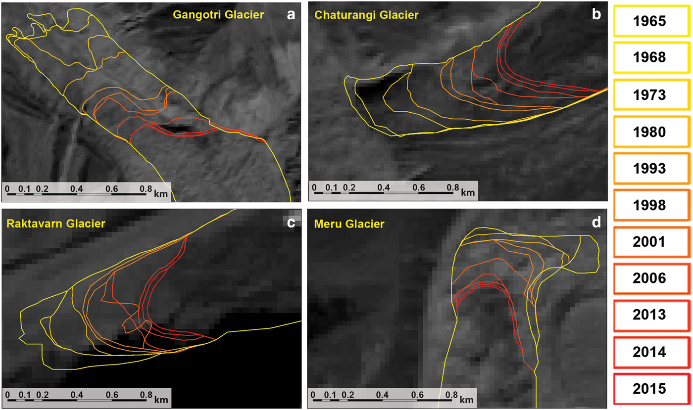
Fig. 4. Gangotri and its tributary glaciers outlines derived from different high-resolution satellite data overlay on Landsat 8 (2013) imagery. Image shows retreat of glacier termini up to ~890, ~678, ~394 and ~378 m for Gangotri, Chaturangi, Raktavarn and Meru glaciers respectively during 1965–2015.
5.2. Glacier length change calculation
Lines with 50 m separation, parallel to the main flow direction of the glacier, were drawn to calculate the length change of Gangotri and its tributary glaciers (Koblet and others, Reference Koblet2010; Bhambri and others, Reference Bhambri, Bolch and Chaujar2012). Length change was calculated as the average change in distance between two consecutive glacier outlines measured from the intersections of the lines with the glacier outlines. We also calculated length changes in terms of the retreat along the central flow line in order to compare with results derived from average length change from the intersection of the lines with the glacier outlines. Based on the outlines of the different years, the area vacated near the snout for Gangotri and its tributary glaciers were calculated (Fig. 4).
5.3. KH-4A Corona DTM processing
A KH-4A Corona DTM for the year 1968 was generated using the Remote Sensing Software Package Graz (RSG) with a fixed focal length of 609.60 mm. Four combinations of forward and aft looking subsets were processed separately in order to accommodate the entire Gangotri and its tributary glaciers. GCPs were collected from terrain corrected Landsat 7 ETM+ imagery (15 m panchromatic band, dated 15 and 22 October 1999) with SRTM3 as vertical reference. In order to improve the sensor model, on average ~ 225 automatically selected tie points (TPs) for each pair of strips were also used (Supplement Table 3). The stereo pairs of all the strips were processed with a RMS of triangulation of <~4 Pixels (Supplement Table 3).
In order to assess glacier changes the DTMs should be carefully co-registered so that all the pixels in the DTMs represent the same location and the elevation deviations of the stable terrain are minimized (Pieczonka and others, Reference Pieczonka, Bolch, Wie and Liu2013). We chose 2006 ASTER as the master/reference DTM. KH-4A DTM (slave) was co-registered following the approach described by Nuth and Kääb (Reference Nuth and Kääb2011) and corrected using global trend surface analysis over gently inclined non-glaciarized terrain using the method described by Bolch and others (Reference Bolch, Buchroithner, Pieczonka and Kunert2008a) and, Pieczonka and others (Reference Pieczonka, Bolch, Wie and Liu2013). The KH-4A DTM was resampled bilinearly to the pixel size of the ASTER DTM (30 m) in order to reduce the effect of different resolutions (Paul, Reference Paul2008; Gardelle and others, Reference Gardelle, Berthier, Arnaud and Kääb2013). After co-registration all the DTM strips were then mosaicked for mass-budget estimation. Before mosaicing, the histograms of the overlapped regions were examined visually and statistically by performing a statistical significance test. For all the overlapping regions the shape of the histograms, mean and SD values were similar and differences between the height values estimated from different corona strips were also statistically insignificant (p = 0.18, 0.21 and 0.02 respectively for three overlapping regions from North). The mosaic operation has been performed in ArcGIS 10.1.
5.4. Terra ASTER DTM processing
ASTER DTMs for the year 2006 and 2014 were generated using PCI Geomatica Orthoengine 2014 selecting the Toutin's model (Toutin, Reference Toutin2002). A sufficient number of well distributed GCPs were selected in a similar way as mentioned in Corona DTM processing (47 and 55 for 2006 and 2014 respectively). All stereo pairs were processed with an RMS of triangulation of <~1 Pixel (Supplementary Table 3). A total of 70 and 65 TPs were used to improve the sensor models for the 2006 and 2014 DTMs respectively. The 2014 ASTER DTM was co-registered with the 2006 ASTER DTM using the same approach described above. The overall quality of the generated raw DTMs appeared promising as most of the glacier parts were almost fully represented. Data gaps mainly occur due to snow cover, cloud cover and cast shadows. The difference images of the DTMs of Gangotri and its tributary glaciers are shown in Figure 5. Elevation differences of the off glacier terrain with ±50 scale of the study area are provided in Supplementary Figure 1.
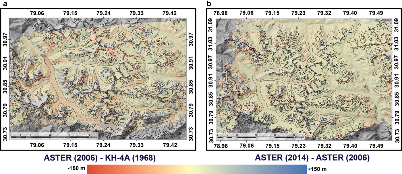
Fig. 5. Total glacier thinning shown as difference image of respective DTMs during the period (a) 2006–1968 and (b) 2014–2006.
5.5. Data gaps and outlier handling
Data gaps in DTMs mainly occur for optical images in the areas with less image contrast. In high-mountain areas this is mainly related to the snow-covered accumulation regions, areas with cast shadows and areas with cloud cover. Therefore, outlier filtering for non-glacierized and glacierized terrain is essential. For the non-glacierized terrain, outliers are defined by the 1.5-fold interquartile range. The 68.3% quantile of the absolute elevation differences over stable terrain was also calculated (Pieczonka and others, Reference Pieczonka, Bolch, Wie and Liu2013) in order to take non-normality into account. The statistics for non-glacierized terrain are shown in Table 1.
Table 1. Stable terrain statistics before and after co-registration (co-registration by Nuth and Kääb, Reference Nuth and Kääb2011; Pieczonka and others, Reference Pieczonka, Bolch, Wie and Liu2013)
NMAD, normalized median absolute deviation; SD, standard deviation; Q68.3, 68.3% quantile.
The thickness changes over the entire glaciers were not homogeneous. It is well-known fact that there is lowest surface elevation change at higher altitude accumulation part of the glacier and maximum lowering in the glacier front for retreating glaciers (Schwitter and Raymond, Reference Schwitter and Raymond1993; Huss and others, Reference Huss, Jouvet, Farinotti and Bauder2010). Therefore, it is not suitable to apply same threshold value for accumulation and ablation region in order to identify the outliers (Pieczonka and Bolch, Reference Pieczonka and Bolch2015). Keeping this in mind, the outliers for glacierized terrain were removed by using an elevation dependent sigmoid function considering the nonlinear behaviour of glacier thickness change. The maximum allowable thickness change (Δh MAX ) corresponding to a certain glacier elevation (E glacier) was calculated by using the following equation as mentioned by Pieczonka and Bolch (Reference Pieczonka and Bolch2015).
 $$\Delta h_{MAX} = \left[ {5 - 5\tanh \left\{ {2\pi - 5\left( {\displaystyle{{E_{MAX} - E_{MIN}} \over {E_{GLACIER}}}} \right)} \right\}} \right] \times STD_{GLACIER}.$$
Where, E MAX and E MIN are the maximum and minimum elevation respectively, E GLACIER is the glacier elevation and STD GLACIER is the overall standard deviation of the glacier elevation differences. All values outside this range have been filtered out as erroneous elevations. Finally, all data gaps in the ablation and accumulation regions were filled by means of ordinary kriging. We have used ordinary kriging because it is more logical to assume a constant mean in the local neighbourhood of each estimation point rather than a constant mean for entire region. Moreover, we also assumed an isotropic nature of the data with stationary variance in order to simplify the model fitting (Li and Heap, Reference Li and Heap2008).
5.6. Mapping uncertainty
Glacier outlines derived from various satellite datasets with different spatial resolutions, acquired at different times with varying snow cover, cloud and shadow conditions have different levels of accuracy. Uncertainty was therefore estimated for all pairs of data used for length estimation. In this study, orthorectified KH-4A Corona (1965 and 1968) and KH-9 Hexagon data (1973 and 1980) were generated using the GCPs collected from terrain corrected Landsat 7 ETM+ imageries (15–10–1999 and 22–10–1999, 15 m panchromatic band) with SRTM3 as vertical reference in RSG and ERDAS LPS Photogrammetry software respectively. Sufficient numbers of GCPs were collected (Supplementary Table 3) and same GCPs were used if they were identifiable in both images. Similarly, ASTER data (2006 and 2014) were orthorectified in PCI Geomatica Orthoengine 2014 using the same GCPs and SRTM3 DTM. The length uncertainty (U L) of each pair of data was calculated from the following formula (Hall and others, Reference Hall, Bayr, Schöner, Bindschadler and Chien2003).
 $$U_{\rm L} = \sqrt {{\left( {R_1} \right)}^2 + {\left( {R_2} \right)}^2} + {\rm RE}$$
where, R 1 and R 2 are the spatial resolution of the image 1 and image 2 respectively and RE is the rectification uncertainty. All the imageries were rectified with KH-4 Corona (1965) image. The uncertainties estimated for all data pairs are given in Table 2.
Table 2. Overall mapping uncertainty determined in this study (Hall and others, Reference Hall, Bayr, Schöner, Bindschadler and Chien2003)
A mapping inaccuracy of 2 pixels was assumed for the outlines derived from KH-4A Corona data (~4 m spatial resolution), mapping inaccuracy of 1 pixel was assumed for KH-9 data (~8 m spatial resolution), ASTER (~15 m spatial resolution) and Landsat OLI (~15 m spatial resolution) and mapping inaccuracy of half a pixel was assumed for Landsat TM data (30 m spatial resolution). This led to an uncertainty of 2.5% for the 1965 KH-4A Corona imagery and 3.1% for the 2015 Landsat 8 data. The overall uncertainty for the area change was 4.0% considering the law of error propagation (Pieczonka and Bolch, Reference Pieczonka and Bolch2015).
5.7. Mass-budget uncertainty
The overall mass-budget uncertainty was estimated by assessing the quality of the elevation products over glacierized as well as non-glacierized terrain. Due to the presence of outliers, normalized median absolute deviation (NMAD) was considered instead of standard deviation (SD) for the quality criteria. However, the NMAD values for all cases (Table 1) over stable terrain differ significantly with the 68.3% quantile. Therefore, considering the non-normality of the elevation differences, the 68.3% quantile was used as the quality criterion for glacier thickness change measurements. Finally, the overall mass budget uncertainty (U M) was calculated using Eq. 3 (Pieczonka and Bolch, Reference Pieczonka and Bolch2015).
 $$U_{\rm M} = \sqrt {{\left( {\displaystyle{{\Delta h} \over t} \times \displaystyle{{\Delta \rho} \over {\rho _{\rm w}}}} \right)}^2 + {\left( {\displaystyle{{U_{DTM}} \over t} \times \displaystyle{{\rho _I} \over {\rho _{\rm w}}}} \right)}^2}. $$
where, Δh is the measured glacier thickness change, t is the observation period, ρw is the density of water (999.972 kg m−3). U DTM is the overall thickness change uncertainty which was assumed to be the 68.3% quantile value. The ice density (ρI) and ice density uncertainty (Δρ) were considered as 850 and 60 kg m−3 respectively (cf. Huss, Reference Huss2013).
5.8. Multitemporal velocity estimation
Surface velocities of the Gangotri Glacier were calculated from multi-temporal Landsat (TM, ETM+, OLI) and ASTER 3N data from 1993 to 2014 using Cosi-Corr (Leprince and others, Reference Leprince, Barbot, Ayoub and Avouac2007). Cosi-Corr is widely used to measure glacier surface velocity for pushbroom sensors like SPOT and ASTER. Landsat data have some advantages over ASTER. For example, it covers an area ~9 times bigger than ASTER and is available from early 1970s, whereas ASTER data is only available from 2000. Landsat data are however, affected by sub-pixel noise created by unknown attitude variation of the satellites and imaging systems (Scherler and others, Reference Scherler, Leprince and Strecker2008). Nevertheless, image to image registration accuracy of ~5 m for ETM+ sensor and ~6 m for TM sensor have been obtained by Lee and others (Reference Lee, Storey, Choate and Hayes2004) and Storey and Choate, (Reference Storey and Choate2004) respectively, which can be considered within an acceptable limit because in most cases the displacements of the glaciological features exceed this noise level (Heid and Kääb, Reference Heid and Kääb2012). Moreover, to compare the results obtained in Cosi-Corr, glacier surface velocity was also estimated using another normalized cross-correlation (NCC) algorithm implemented on Correlation Image Analysis Software (CIAS) (Kääb and Vollmer, Reference Kääb and Vollmer2000) for the period 1993/94 (Fig. 6). Surface velocity along the central flow line estimated from both the software was quite similar (p = 0.44). Therefore, glacier surface velocities were estimated using Cosi-Corr for the remaining dataset.
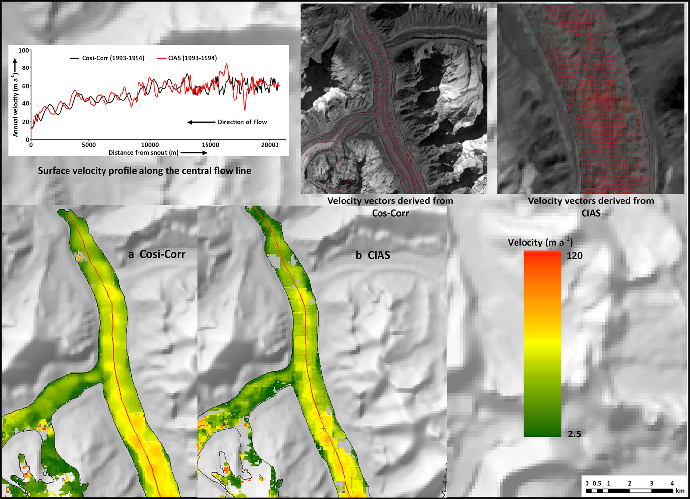
Fig. 6. Velocity image of Gangotri Glacier System derived from images acquired on 29 October 1993 and 17 November 1994 based on correlation of ortho images in Cosi-Corr and in CIAS software. Graph shows the velocity profile along the central flow line (Red line marked in the image). The arrow lengths for both the images are not in the same scale.
The correlation analysis was performed using different window sizes and steps for different datasets. Initially a rough pixel-wise displacement was estimated using bigger window size followed by the sub-pixel displacement determination using smaller window size (Leprince and others, Reference Leprince, Barbot, Ayoub and Avouac2007). Initial and final window sizes of 64 and 32 pixels with a step of 2 pixels were used for Landsat TM and ETM+ data whereas a window size of 128 and 32 pixels with a step of 4 pixels were used for ASTER 3N and Landsat 8 dataset to achieve an ice flow velocity map sampled at every 60 m.
The correlation images were filtered to exclude miscorrelation using three filtering steps. Initially low SNR pixels (SNR ≤ 0.90) were excluded from the displacement map. Then the pixels whose velocity direction deviated ± 200 from the glacier flow direction were removed by using a directional filter (Kääb, Reference Kääb2005; Kääb and others, Reference Kääb, Lefauconnier and Melvold2005). Finally, a magnitude filter was also used, considering the fact that the velocities do not change abruptly, but rather, gradually (Scherler and others, Reference Scherler, Leprince and Strecker2008).
6. RESULTS
6.1. Length and area vacated near snout
This study revealed that Gangotri Glacier retreated ~889.4 ± 23.2 m with an average rate of 17.9 ± 0.5 m a−1 from 1965 to 2015 (Table 3). Variable retreat rates can be observed during the entire observational period for the Gangotri Glacier. The retreat rate was considerably lower between 1965 and 1968 but then increased during 1968–1973. However, in recent years (2006–15) the retreat rate was lower (~9.0 ± 3.5 m a−1) as compared with the period 1965–2006 (~19.7 ± 0.6 m a−1). Mean annual retreat of 0.9% could be observed during recent years (2006–15) whereas the rate was significantly higher (~2.2%) between 1965 and 2006. Fluctuation of snout position was also estimated along the central flow line and found to be higher than that measured by averaging along the front. Slightly lower average retreats were estimated for the tributary glaciers (Table 3).
Table 3. Total and average recession of Gangotri and its selected tributary glaciers length
The area of Gangotri Glacier near its snout, considering areas upto ~2 km from the snout position, delineated from the year 1965, shrank by 0.47 ± 0.07 km2 with an average of 0.01 ± 0.001 km2 a−1 (0.33 ± 0.02%) between 1965 and 2015 (Table 4). Similar to the measured retreat rate, the rate of area loss near the snout of Gangotri Glacier decreased during the period of 2006–15 and was found to be 0.006 ± 0.002 km2 a−1 (0.04 ± 0.01%), whereas from 1965 to 2006 the area shrinkage rate was 0.01 ± 0.001 km2 a−1 (0.3 ± 0.02%). The total debris-covered area was 25.5 ± 1.0 km2 (~17.9 ± 0.7% of the whole ice cover) in 1965 which increased to 38.7 ± 2.9 km2 (~27.3 ± 2.0% of the whole ice cover) in 2015. Debris cover significantly increased during recent time. During 1965–2006 and 2006–15 overall debris cover increased by ~4.4 ± 0.9% (~0.15 ± 0.03 km2 a−1) and ~4.9 ± 1.2% (0.8 ± 0.2 km2 a−1) respectively.
Table 4. Total and average area vacated near snout of Gangotri and its selected tributary glaciers
6.2. Glacier mass budget
Gangotri and its tributary glaciers experienced predominant downwasting between 1968 and 2014 with an average thickness decrease of 10.5 ± 7.2 m resulting in an average mass loss of 0.19 ± 0.12 m w.e. a−1 (Table 5). The highest mass loss could be observed during the period 2006–14 with an average mass budget of −0.29 ± 0.19 m w.e. a−1. However, the mass loss rate during the period 1968–2006 was less as compared with the recent period and found to be 0.17 ± 0.12 m w.e. a−1. Average surface lowering along longitudinal profiles with normalized length for Gangotri and its tributary glaciers are shown in Figure 7. The profiles are generated by applying a moving average with a bandwidth of 150 m. Our results indicate an increased surface lowering rate of Gangotri and its tributary glaciers could be found during 2006–14 period (0.34 ± 0.2 m a−1) as compared with 1968–2006 period (0.20 ± 0.1 m a−1). However, the differences are not significant. Significant surface lowering in the debris-covered glacier part only could be observed for the Gangotri Glacier main trunk (Fig. 8). The average surface lowering rate in the debris-covered part of the Gangotri main trunk were 0.54 ± 0.3 m a−1 (1968–2006) and 0.8 ± 0.6 m a−1 (2006–14), clearly indicating that significant thickness loss occurred despite thick debris cover. Our results indicate that the debris-free region also thinned during the investigated time. A slight thickening, especially in the accumulation region of Gangotri and Raktavarn glaciers (Fig. 7) in recent years (2006–14) is observed, possibly caused by an increase in the amount of precipitation. However considering the high uncertainty, detailed analyses of meteorological data are required to validate the statement, which are not available with us.
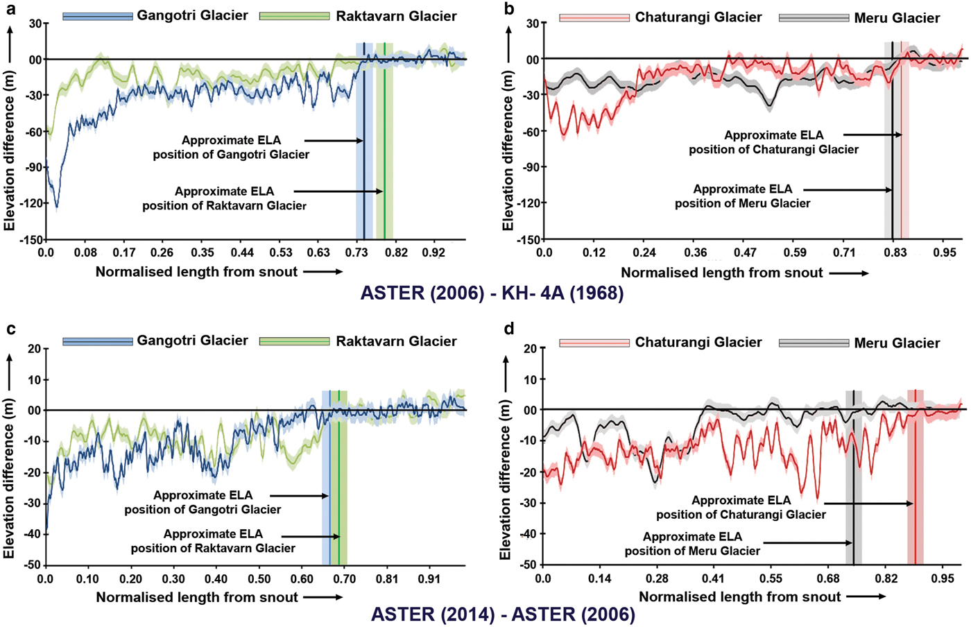
Fig. 7. Thickness change along longitudinal profile with normalized length. During 2006–1968 (a) Gangotri and Raktavarn Glaciers (b) Chaturangi and Meru Glaciers, and during 2014–2006 (c) Gangotri and Raktavarn Glaciers (d) Chaturangi and Meru Glaciers. The profiles are generated applying a moving average with a bandwidth of 150 m. Light colour seam along the profile lines indicate 68.3% quantile of the absolute elevation difference.
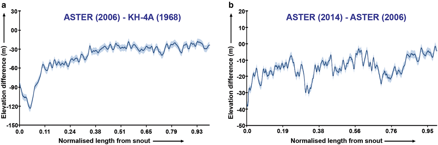
Fig. 8. Thickness change of debris cover region along longitudinal profile of Gangotri Glacier main trunk during (a) 2006–1968 (b) 2014–2006. The profiles are generated applying a moving average with a bandwidth of 150 m. Light colour seam along the profile lines indicate 68.3% quantile of the absolute elevation difference.
Table 5. Mass loss and surface lowering during 1968–2014 of Gangotri and its selected tributary glaciers
6.3. Glacier surface velocity
The velocity measurements using Cosi-Corr show that Gangotri Glacier is active throughout the tongue but the velocity varied slightly from 1993 to 2014 (Fig. 9). We picked a profile along the central flow line of the Gangotri Glacier main trunk and plotted the annual velocity (Fig. 10). We extracted the displacement data along a profile that extends from the accumulation zone, down to the toe of the glacier. Due to the lack of visible surface features in the snow covered region the correlation was not satisfactory. However, annual displacement profiles in the lower regions were consistent and the standard deviation among data points from different displacement profiles were ~7 m a−1, except the 1996/97 displacement (~11 m a−1).
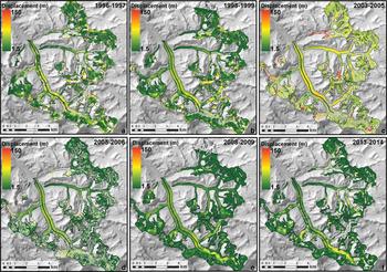
Fig. 9. Displacement image of Gangotri Glacier System derived from correlation of ortho images acquired on (a) 14 October 1996–22 September 1997 (b) 11 October 1998–15 October 1998 (c) 10 October 2003–15 October 2005 (d) 15 October 2005–9 October 2006 (e) 23 November 2008–26 November 2009 and (f) 29 October 2013–17 November 2014.
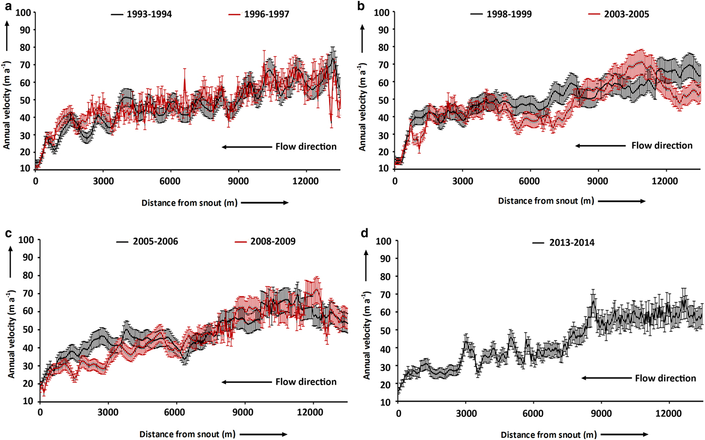
Fig. 10. Comparison of annual velocity profile in different years along the central flow line of Gangotri Glacier main trunk.
Annual surface velocities during 1998/99 (average velocity ~50 ± 7.2 m a−1) were slightly higher compared with the 1993/94 period (average velocity ~46 ± 7.5 m a−1). It can be assumed that higher surface velocities are probably associated with higher temperatures during that period or more precipitation in the previous years. No significant annual velocity trends were visible in most parts of the central flow line, except some portion of the ablation region during 1996/97 (Fig. 9). The average surface velocity after the October 1999 (~46 ± 5.5 m a−1) was found to be slightly less than before.
Velocity differences in the debris-covered region between 2003–05 and 2005/06 were insignificant (p = 0.1) and almost indistinguishable. The differences during the years 2008/09 and 2013/14 were also insignificant (p = 0.1). However, significant differences (p = 0.001) in the debris-covered region can be observed by comparing 2003–05 and 2005/06 with 2008/09 and 2013/14.
The annual surface velocity between 2008 and 2009 (~48 ± 4.8 m a−1) was slightly higher compared with the 2013/14 period (~43 ± 5.1 m a−1) and that in the 2003–06 period was slightly higher (~48 ± 6.1 m a−1) than in the 2008–14 period (~42 ± 4.9 m a−1) (Fig. 10). The average velocity during 2006–14 (~44.7 ± 4.9 m a−1) decreased by ~6.7% as compared with that during 1993–2006 (~48.1 ± 7.2 m a−1). Our results provide an indication that the glacier velocity might have slightly decreased but the differences are not significant.
7. DISCUSSION
7.1. Glacier length and area change near snout
Gangotri Glacier has been studied extensively in terms of its retreat rates. Estimated retreat rate and associated uncertainty vary considerably in most of the studies due to inconsistencies of the methods used. The majority of remote sensing-based studies have used topographic maps provided by the Survey of India (SOI) or coarse-resolution satellite data. The retreat rate of the Gangotri Glacier is significantly lower as compared with some previous estimation where 1962 topography map was used. For instance, an average retreat rate of ~38 m a−1 (total ~1651 m) between 1962 and 2006 was reported by Bhambri and Chaujar, (Reference Bhambri and Chaujar2009) using topography map (1962) and ASTER data (2006). Similarly, Tangari and others (Reference Tangari, Chandra, Yadav, Srivastava, Gupta and Mukerji2004) reported ~1600 m (~42 m a−1) recession of Gangotri Glacier using 1962 topography map and IRS-1D data between 1962 and 2000. 1962 SOI topography map and IRS-1C data (2000) were also used by Bahuguna and others (Reference Bahuguna2007) to estimate recession of Gangotri Glacier and it was found to be ~1510 m (~40 m a−1). Several studies highlighted overestimated delineation of glacier outline in 1962 SOI topographic map (Vohra, Reference Vohra1980; Raina and Srivastava, Reference Raina and Srivastava2008; Raina, Reference Raina2009 etc.). Therefore, it can be assumed that the higher retreat of Gangotri Glacier is probably associated with the inconsistency of the SOI map.
On the contrary, our estimated retreat rate is in good agreement with several other published results, where mainly satellite data were used for retreat estimation. An average retreat rate (~20 m a−1) similar to this study (~17.9 ± 0.5 m a−1) was reported (Fig. 2 and Supplementary Table 1) in literatures during different time periods (Kumar and others, Reference Kumar, Areendran and Rao2009; Kargel and others, Reference Kargel, Cogley, Leonard, Haritashya and Byers2011; Saraswat and others, Reference Saraswat2013 etc.). Moreover, total and average retreat (~739.7 ± 27.5 m and ~22.4 ± 0.8 m a−1) of Gangotri Glacier during 1968–001 using low resolution ASTER data was supported by the results obtained by using high resolution IRS-1C PAN data (~764 ± 19 m and ~23.2 ± 0.6 m a−1) by Bhambri and others (Reference Bhambri, Bolch and Chaujar2012). An overestimated recession of Gangotri Glacier along the central flow line (~1057.1 ± 23.2 m) could be observed during the entire observation period as compared with the retreat calculated from the intersection of the glacier outlines with the lines drawn parallel to the central flow line (~889.4 ± 23.2 m). Thus, measurements based along the centre flow line might not provide clear evidence of overall retreat of the glacier tongue. Therefore, averaging along the front is a more robust method, which was already mentioned by Bhambri and others (Reference Bhambri, Bolch and Chaujar2012), and provides more reliable estimations. The centre portion of the terminus of Gangotri Glacier advanced slightly during 1968, but the averaging along the entire glacier front during the period between 1965 and 1968 clearly indicated significant retreat (−6.7 ± 3.7 m a−1).
This study demonstrated that Gangotri Glacier lost an area of 0.47 ± 0.03 km2 (~0.01 ± 0.001 km2 a−1) between 1965 and 2015 from its front. These results match well with the remote sensing based study by Bhambri and others (Reference Bhambri, Bolch and Chaujar2012) and also with the study conducted by GSI using in-situ field surveys by Srivastava (Reference Srivastava, Srivastava, Gupta and Mukerji2004). Observation was taken from 1965 to 2006 by Bhambri and others (Reference Bhambri, Bolch and Chaujar2012) using high-resolution satellite imageries (KH-4, KH-9, IRS-1C and Cartosat-1) and it was found that 0.41 ± 0.03 km2 (~0.01 km2 a−1) area was vacated near the snout of Gangotri Glacier. GSI study suggested 0.58 km2 (~0.01 km2 a−1) area lost near the snout from 1935 to 1996. Moreover, during 1968–2006 the area vacated near snout of Gangotri Glacier (0.39 ± 0.03 km2 and ~0.01 ± 0.007 km2 a−1) estimated from our study was also supported by Bhambri and others (Reference Bhambri, Bolch, Chaujar and Kulshreshta2011a) during the same observation period (0.38 ± 0.03 km2 and 0.01 km2 a−1) by using KH-4 and Cartosat-1 data. However, the area loss during 2001–06 found in our study is slightly higher (~0.007 ± 0.003 km2 a−1) as compared with the findings of Bhambri and others (Reference Bhambri, Bolch and Chaujar2012) (0.003 ± 0.002 km2 a−1). The difference is probably due to the use of coarser resolution ASTER data compared with IRS PAN and Cartosat-1 data. However, the results are within the uncertainty range. Compared with other parts of Garhwal Himalaya, the shrink rate of Gangotri Glacier from this study was slightly higher (~0.01 ± 0.001 km2 a−1) during 1965–2015. For instance, Satopanth Glacier and Bhagirathi Kharak Glacier shrank by 0.314 km2 (~0.007 km2 a−1) and 0.129 km2 (~0.002 km2 a−1) near their snouts between 1962 and 2006 (Nainwal and others, Reference Nainwal, Negi, Chaudhary, Sajwan and Gaurav2008). Similar values for Satopanth Glacier and Bhagirathi Kharak Glacier were also estimated by Bhambri and others (Reference Bhambri, Bolch, Chaujar and Kulshreshta2011a) based on Corona and ASTER imagery during 1968–2006. In addition, Pindari Glacier, Uttarakhand, lost 0.111 km2 (~0.0026 km2 a−1) at its front during 1958–2001 determined by Oberoi and others (Reference Oberoi, Maruthi and Siddiqui2000).
Several other studies have reported that debris cover increased over time in the Himalaya (Iwata and others, Reference Iwata, Aoki, Kadota, Seko, Yamaguchi, Nakawo, Raymond and Fountain2000; Bolch and others, Reference Bolch, Buchroithner, Pieczonka and Kunert2008a; Kamp and others, Reference Kamp, Byrne and Bolch2011). Our study also estimated that the debris cover area of the Gangotri Glacier main trunk increased significantly by 13.1 ± 2.1 km2 or 9.2 ± 1.2% (~0.2 ± 0.03% a−1) between 1965 and 2014, which is similar to Bhambri and others (Reference Bhambri, Bolch, Chaujar and Kulshreshta2011a) who found that an area in upper Bhagirathi Basin increased by 11.8 ± 3.0% (~0.31 ± 0.08% a−1) during 1968–2006. Bhambri and others (Reference Bhambri, Bolch, Chaujar and Kulshreshta2011a) also estimated that ~ 83% of the upper Bhagirathi Basin is covered by three large debris covered glaciers: Gangotri, Raktavarn and Chaturangi. This study also supports the above mentioned findings for the Gangotri Glacier during 1965–2014.
7.2. Glacier mass change
The mass-balance patterns in the Hindu Kush Himalayan (HKH) region are highly variable due to the wide variation of climatic conditions, different glacier features and different geographic regions (Bolch and others, Reference Bolch2012; Gardelle and others, Reference Gardelle, Berthier, Arnaud and Kääb2013; Kääb and others, Reference Kääb, Treichler, Nuth and Berthier2015). For instance, a slight mass gain or balanced mass budget was observed in the central Karakoram region, whereas moderate to high-mass loss were observed in the Central/Eastern Himalaya and Western Himalaya respectively during the recent decade (Azam and others, Reference Azam2012; Gardelle and others, Reference Gardelle, Berthier, Arnaud and Kääb2013; Vincent and others, Reference Vincent2013). However, to our knowledge no mass-balance study has been published in peer-reviewed literature for Gangotri Glacier to date and mass-balance data in the Himalayan region become sparser as we go back in time (Bolch and others, Reference Bolch2012). Thus, the rate at which these glaciers are changing remains poorly understood. This study presents the longest mass-balance study using remote sensing techniques for Gangotri Glacier and indicates that the mass loss of Gangotri and its tributary glaciers (0.19 ± 0.12 m w.e. a−1) from 1968 to 2014 is slightly less than reported for other debris-covered glaciers in Himalayan regions. For instance, in-situ measurements by Dobhal and others (Reference Dobhal, Gergan and Thayyen2008) for Dokriani Glacier (area ~7 km2, length ~5 km and ~20% debris cover) in the Garhwal Himalaya, from 1992 to 2000 revealed a mass loss of 0.32 m w.e. a−1. Gautam and Mukherjee (Reference Gautam and Mukherjee1989) estimated mass lost of 0.24 m w.e. a−1 during 1981–88 for Tipra Glacier (area ~7.5 km2, length ~7 km, thick debris cover). Moreover, various mass-balance studies were also conducted for nearly debris-free Chhota Shigri Glacier (area ~15.7 km2, length ~9 km) in Himachal Pradesh using different techniques. For example, Azam and others (Reference Azam2012) estimated mass loss of 0.67 ± 0.40 m w.e. a−1 during 2002–10 using glaciological method and field investigation. Later on, Vincent and others (Reference Vincent2013) compared these results with geodetic measurements and found a lower mass loss rate of 0.44 ± 0.16 m w.e. a−1 during 1999/–10.
Geodetic assessments showed a mass loss of 0.33 ± 0.18 m w.e. a−1 for the heavily debris covered glaciers (Lirung Glacier, area ~6.4 km2; Shalbachum Glacier, area ~11.5 km2; Langtang Glacier, area ~53.5 km2 and Langshisha glacier, area ~23.5 km2) in the upper Langtang valley, central Himalaya, Nepal, during 1974–99 (Pellicciotti and others, Reference Pellicciotti2015). A similar value during 1970–2007 (0.32 ± 0.08 m w.e. a−1) was also observed by Bolch and others (Reference Bolch, Pieczonka and Benn2011) for ten glaciers (nine out of them were heavily debris covered having debris area ~36.3 km2), south and west of Mount Everest using stereo Corona imageries, aerial images and high-resolution Cartosat-1 data. However, the debris covered Khumbu Glacier (length ~12 km) in this region lost 0.27 ± 0.08 m w.e. a−1 during the same period (Bolch and others, Reference Bolch, Pieczonka and Benn2011). It is worth mentioning that, in spite of the lower overall mass budget during the observation period of Gangotri and its tributary glaciers, significant surface lowering could be observed in the debris-covered part only.
Our study also estimated slope variations of Gangotri and its tributary glaciers (Fig. 11) to interpret the thinning characteristics, as mentioned by several researchers (Nuimura and others, Reference Nuimura, Fujita, Yamaguchi and Sharma2012; Pellicciotti and others, Reference Pellicciotti2015). Five length profiles parallel to the central flow line were drawn and the mean values were considered in order to avoid the ambiguous selection of the central flow line (Pellicciotti and others, Reference Pellicciotti2015). Nuimura and others (Reference Nuimura, Fujita, Yamaguchi and Sharma2012) observed higher surface lowering of debris cover part in lower mean slope for large glaciers and vice-versa for small glaciers in the Khumbu region. They also mentioned that the debris covered glacier can absorb large amounts of energy (Sakai and others, Reference Sakai, Nakawo and Fujita2002) due to the presence of supraglacial ponds and ice cliffs, which may increase melting rate (Pellicciotti and others, Reference Pellicciotti2015). Very rough topography (Fig. 11) and the presence of numerous supraglacial ponds on the debris covered portion of the Gangotri Glacier were also confirmed by Bhambri and others (Reference Bhambri, Bolch, Chaujar and Kulshreshta2011a). Nuimura and others (Reference Nuimura, Fujita, Yamaguchi and Sharma2012) also observed that the higher mass loss rate in debris covered region occurred in moderate slope as compared with steep slopes. A similar conclusion was also drawn by Pellicciotti and others (Reference Pellicciotti2015) from their analysis of the glaciers in the upper Langtang valley. It is also evident from our study that for all glaciers, thinning is stronger for the gentler slopes, especially in the lower sections of the tongues.
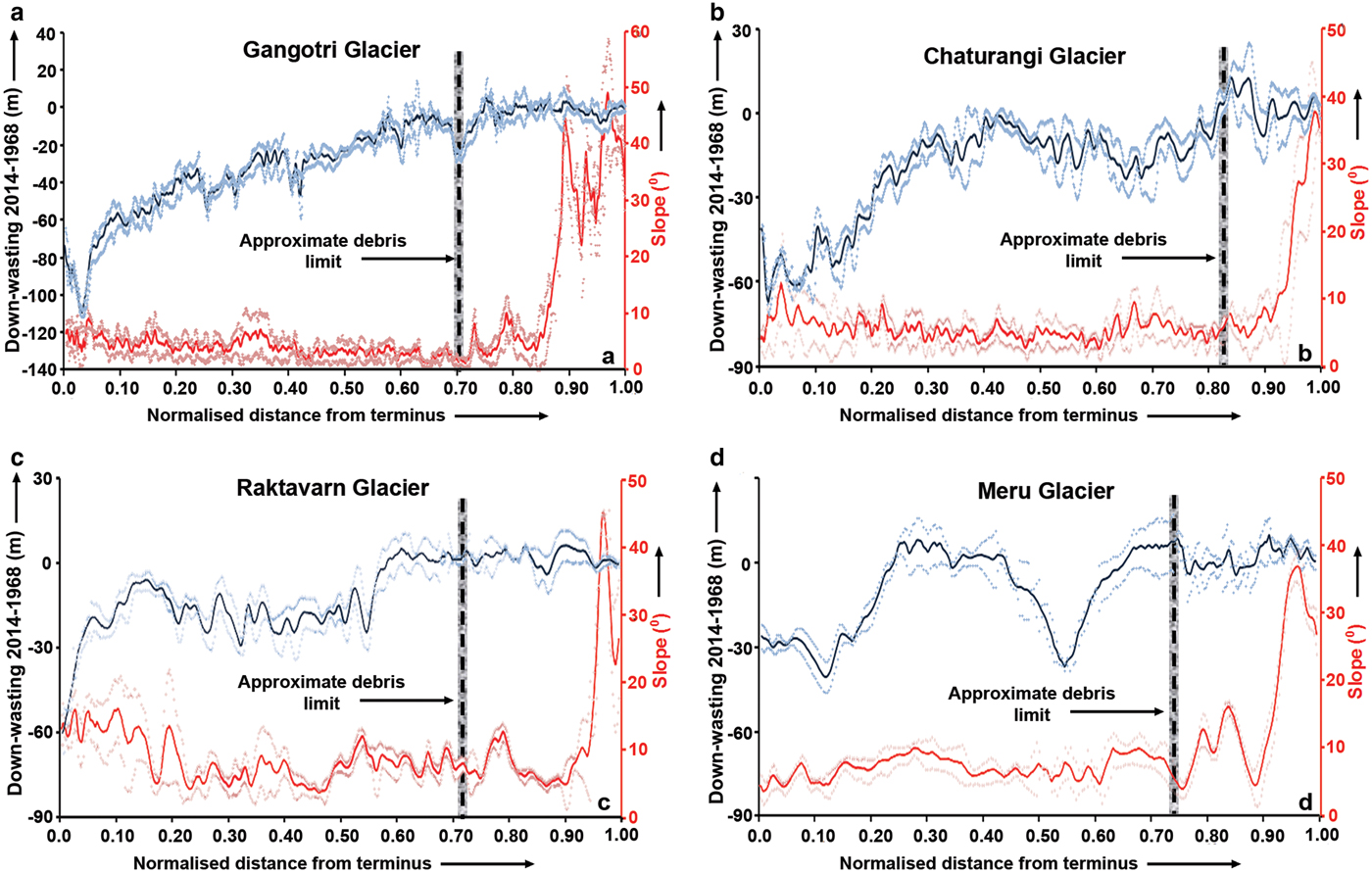
Fig. 11. Normalized length profiles with average elevation difference during the period 2014–1968 (blue) and average slope estimated from SRTM (orange), where the average results are from five parallel length profiles for each of the four glaciers: (a) Gangotri Glacier (b) Chaturangi Glacier (c) Raktavarn Glacier and (d) Meru Glacier. Uncertainty range is the standard deviation (dotted); approximate debris limits (vertical line). Curves of both elevation changes and slope were smoothed with a five-window moving average.
7.3. Glacier surface velocity
So far, few studies have investigated the velocity of the Gangotri Glacier in different time periods. Scherler and others (Reference Scherler, Leprince and Strecker2008) observed an increasing glacier surface flow velocity with distance upstream from the terminus of the debris-covered Gangotri Glacier using normalized cross-correlation of optical imageries. Gantayat and others (Reference Gantayat, Kulkarni and Srinivasan2014) reported that the maximum velocity varied from ~61 to ~85 m a−1, whereas minimum velocity varied from ~5 to ~15 m a−1 for the Gangotri Glacier main trunk during 2009/10 using Landsat TM data. Similar results were also reported for Gangotri Glacier using ASTER data by Saraswat and others (Reference Saraswat2013). They reported that the velocity decreased from ~70.2 ± 2.3 m a−1 to <~30 ± 2.3 m a−1 from the accumulation to the ablation region during 2009/10. Our analysis during 2008/09 also produced similar values (maximum ~71 m a−1 and minimum ~13 m a−1). Glacier surface velocities were also estimated in different parts of the Himalayan region. For instance, Müller (Reference Müller1968) estimated the surface velocity of the Khumbu Glacier during April 1956 to November 1956 at the Everest Base Camp (EBC) and found ~58 m a−1 whereas surface velocity was ~28 m a−1 at the transition between clean ice and debris-covered ice. Bolch and others (Reference Bolch, Buchroithner, Peters, Baessler and Bajracharya2008b) also estimated glacier surface velocity of the Khumbu Glacier based on the Ikonos (2000/01) and ASTER (2001–03) data. The glacier surface velocity varied from >50 m a−1 to <30 m a−1 in the upper debris-free zone and decreased gradually towards the terminus. Glacier surface velocities of the same glacier were also estimated by Luckman and others (Reference Luckman, Quincey and Bevan2007) using ERS data during 1992–2002 and it was found as ~50 m a−1 at the EBC and <~20 m a−1 south of the transition between clean ice and debris-covered ice.
The glacier surface velocity among the investigated glaciers was also estimated during recent years (2008/09). The average velocity of the Gangotri Glacier was significantly higher (~48 ± 4.8 m a−1) than the Chaturangi Glacier (~20.1 ± 3.7 m a−1) and Raktavarn Glacier (~17.9 ± 4.0 m a−1) whereas, the average velocity of Meru Glacier was in between (~33.6 ± 5.3 m a−1). Gangotri Glacier flow velocity was also monitored during the late 70s using glaciological methods (Srivastava, Reference Srivastava2012). During 1977, average flow velocity near the snout of Gangotri Glacier was estimated as ~44 m a−1 whereas ~33 m a−1 flow velocity was reported at the junction point between Gangotri and Chaturangi Glacier. However, measurements based on one point of the glacier are not representative for the entire glacier.
The processing errors were also examined for the locations of stable ground near the snout of the Gangotri Glacier where the slope conditions were nearly the same as the glacier (Saraswat and others, Reference Saraswat2013). The location of the stable ground and the errors associated with the processing for all pairs of data are shown in the Supplementary Figure 2. The mean bias varies from 1.43 m a−1 (2013/14) to 5.77 m a−1 (2003–05) and the standard deviation varies from 0.63 m a−1 (2013/14) to 3.01 m a−1 (1996/97), which were quite similar to the reported values estimated by Saraswat and others (Reference Saraswat2013) using ASTER dataset from 2005 to 2011 for Gangotri Glacier.
A relationship similar to Pellicciotti and others (Reference Pellicciotti2015) and Holzer and others (Reference Holzer2015) between recent surface velocity (2008/09) and down-wasting during the entire observation period (1968–2014) was also estimated through a profile along the central glacial flow line for all investigated glaciers (Fig. 12). The maximum down-wasting for most of the investigated glaciers in this study can be observed corresponding to lower surface velocities, particularly within few kilometres upward from their respective tongues. Sakai and others (Reference Sakai, Takeuchi, Fujita and Nakawo2000) investigated the importance of supraglacial ponds in ablation process of the debris-covered Lirung Glacier in Langtang valley, Nepal Himalayas. They have reported that the heat absorption rate of a supraglacial pond is ~7 times higher than the average heat absorption of the entire debris-covered region and more than half of the heat is released through the water flow from the supraglacial pond. Heat contained in the water expands the englacial conduit and hence enhance internal ablation. Therefore, it may be inferred from our study also that the considerable down-wasting occurred due to the presence of supraglacial ponds in the tongue, which may absorb large amount of incoming electromagnetic energy (Holzer and others, Reference Holzer2015). Despite strong down-wasting together with lower surface velocity in the lower portion of the glaciers, our study estimated significant retreat rate, though the rate is less in recent time (Table 3). Hence, Gangotri Glacier behaves in this regard differently than other debris-covered glaciers such as Khumbu, Nuptse and Lhotse glaciers at Mount Everest, Nepal (Bolch and others, Reference Bolch, Pieczonka and Benn2011), Fedchenko Glacier in Pamir, Tajikistan (Lambrecht and others, Reference Lambrecht, Mayer, Aizen, Floricioiu and Surazakov2014), and Muztag Ata Glacier in eastern Pamir (Holzer and others, Reference Holzer2015), which appeared to have stagnant debris-covered tongues.
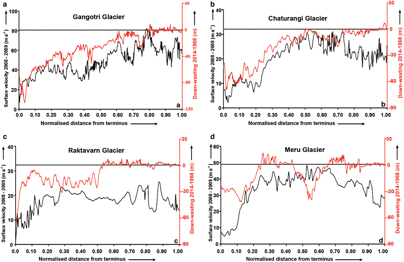
Fig. 12. The profile shows the surface velocities during 2008/09 (black) and corresponding down-wasting during 1968–2014 (red) for each of the four glaciers: (a) Gangotri Glacier (b) Chaturangi Glacier (c) Raktavarn Glacier and (d) Meru Glacier. Flow velocity was measured in upstream direction.
The velocity profile along the central flow line of Gangotri Glacier was critically examined during 2008–10. Significant annual velocity differences along the profile can be observed from October 2008 to July 2009 and from July 2009 to October 2010 (Fig. 13a). Earlier annual velocities along the profile were faster than the most recent. However, it was not clear from the results whether this velocity difference is a true decrease over entire time period or only a seasonal effect. Therefore, seasonal effect was also studied similar to the study mentioned by Scherler and others (Reference Scherler, Leprince and Strecker2008).
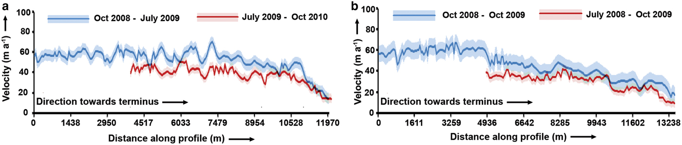
Fig. 13. Annual surface velocity derived from the correlation of ortho-images (Landsat TM L1 T) during (a) October 2008–October 10 and (b) October 2008–October 09. Light blue and light red seam along the profile lines indicate one sigma error. Figure shows the high contribution to the displacement during the summer period. In the upper part of the glacier the red line is missing due to fresh snow cover.
Several studies demonstrated that glacier flow velocities can vary significantly throughout the year (Anderson and others, Reference Anderson2004; Bartholomaus and others, Reference Bartholomaus, Anderson and Anderson2008). Harper and others (Reference Harper, Humphrey, Pfeffer and Lazar2007) mentioned that highest surface velocity for many mountain glaciers can be observed during spring to early summer. In order to examine the seasonal effect of Gangotri Glacier we investigated annual surface velocities along the central flow lines over different periods of 2008–10 as described by Scherler and others (Reference Scherler, Leprince and Strecker2008). A difference in annual surface velocity in lower parts of the glacier along the profile can be observed between the time period starting in July 2008 and in October 2008. The velocity estimated during October 2008/09 was relatively faster than the velocity from July 2008 to October 2009 (Fig. 13b). This difference of surface velocities can be attributed due to the addition of the slow surface velocity period during July–October (Scherler and others, Reference Scherler, Leprince and Strecker2008), when the flow velocity is relatively slower as compared with the average annual velocity. Therefore, it can be assumed that the velocity difference during October 2008 to July 2009 and July 2009 to October 2010 (Fig. 13a) as compared with October 2008 to October 2009 and July 2008 to October 2009 (Fig. 13b) may be due to the effect of slower velocities. Thus it can be concluded from this study that the higher melting and consequent higher surface velocity may occur due to high temperatures during the early summer. Such observations are also reported by meteorological and hydrological studies (Singh and others, Reference Singh, Haritashya, Kumar and Singh2006, Reference Singh, Haritashya and Kumar2007) and remote sensing-based studies (e.g. Scherler and others, Reference Scherler, Leprince and Strecker2008).
8. CONCLUSIONS
We have examined glacier length, area and elevation changes for the Gangotri Glacier and its three major tributaries – Chaturangi Glacier, Raktavarn Glacier and Meru Glacier, Garhwal Himalaya, India – for the last five decades. All four glaciers are heavily debris-covered on their tongues. The seasonal variations of ice surface velocity for the last two decades also have been investigated in this study. Our main conclusions are as follows:
-
(1) The average retreat rate of the Gangotri Glacier during the observed period (1965–2015) was found to be consistent with the other reported values, which used satellite data for comparisons. The retreat rate of Gangotri Glacier declined from 19.7 ± 0.6 m a−1 during 1965–2006 to 9.0 ± 3.5 m a−1 during 2006–15. Rate of retreat in this study, however, estimates less recession as compared with the measurement obtained from 1962 SOI map.
-
(2) This study also demonstrated that significant areas were vacated near the front of Gangotri Glacier during the investigated time. Our study also estimated that the debris cover area of the Gangotri Glacier main trunk increased significantly (~0.2 ± 0.03% a−1) in 2014 as compared to 1965. Maximum average increase could be found during the most recent period of study (2006–15).
-
(3) The mass loss for Gangotri and its tributary glaciers (0.19 ± 0.12 m w.e. a−1) during the observation period was slightly less than those reported for other debris covered glaciers in Himalayan regions. Our observation also revealed that the recent down-wasting (2006–14) was significantly higher than the previous period (1968–2006). Despite the lower overall mass budget during the observation period for Gangotri and its tributary glaciers, significant surface lowering could be observed in debris-covered part. It was also observed that even though the debris-free regions also possibly thinned during the investigated time, there might be a slight thickening in the accumulation region, especially in Gangotri Glacier and Raktavarn Glacier in recent years (2006–14). Our study on Gangotri and its tributary glaciers also support earlier findings in the sense that for debris-covered glaciers thinning is stronger for the gentler slopes, especially in the lower sections of the tongues.
-
(4) Gangotri Glacier loses significantly mass despite thick debris-cover. However, retreat rates in recent years (2006–15) are less as compared with previous years (1965–2006).
-
(5) Our study found a slightly lower surface velocity for Gangotri Glacier after the year 2000 as compared with mid ‘90s. Analysis of surface velocities also revealed that there was a clear reduction in velocities from the accumulation to the ablation region during the entire observation period. The surface velocity of the Gangotri Glacier during 2008/09 was found to be consistent with the other reported values. The maximum down-wasting occurred corresponding to the region of lower surface velocities particularly within 1–2 km upward from their respective tongues. It was also observed that the tongue is active throughout, in contrast to other Himalayan debris-covered glaciers.
SUPPLEMENTARY MATERIAL
To view supplementary material for this article, please visit http://dx.doi.org/10.1017/jog.2016.96.
ACKNOWLEDGEMENTS
A. Bhattacharya acknowledges research funding through Alexander von Humboldt (AvH) foundation and T. Bolch acknowledges funding through the German Research Foundation (DFG, code BO 3199/2–1) and the European Space Agency (Glaciers_cci project. code 400010177810IAM). ASTER data were provided at no cost by NASA/US Geological Survey under the umbrella of the Global Land Ice Measurements from Space (GLIMS) project. The authors acknowledge the USGS Earth Resources Observation and Science Center (EROS) for providing the Landsat imageries. Special thanks are due to two anonymous referees and the scientific editor of the paper for their careful and constructive comments.
AUTHOR CONTRIBUTIONS
A.B. and T.B. designed the study and discussed the results. T.P. and K.M. supported the DTM generation and J.K. the velocity calculation. A.B. performed all analysis, generated the figures and wrote the draft of the manuscript. All authors contributed to the final form of the article.


 Open access