


INTRODUCTION
The majority of the ice in the Antarctic ice-sheet drains from the continent to the ocean through fast-flowing ice streams and outlet glaciers (e.g. Bamber and others, Reference Bamber, Vaughan and Joughin2000; Rignot and others, Reference Rignot, Mouginot and Scheuchl2011). The high velocities of these features are thought to be sustained by the presence of meltwater at the bed, which reduces frictional resistance (e.g. Engelhardt and Kamb, Reference Engelhardt and Kamb1997; Tulaczyk and others, Reference Tulaczyk, Kamb and Engelhardt2000). Thermodynamic ice stream models suggest, however, that in downstream regions of fast flow, where driving stresses are low and ice is thin, the basal temperature regime favors freezing of subglacial water (e.g. Hulbe and MacAyeal, Reference Hulbe and MacAyeal1999). Therefore, sustaining fast ice flow in areas where basal freezing is predicted requires transport of large quantities of subglacial water from upstream areas of basal melt to these downstream regions (e.g. Kamb, Reference Kamb, Alley and Bindschadler2001; Joughin and others, Reference Joughin, Tulaczyk, MacAyeal and Engelhardt2004). This implies that both the location and movement of water at the ice–bed interface are first-order controls on the mass balance of Antarctica.
The movement of water from the upstream melt zones to downstream regions of fast flow has long been thought of as a steady-state process over short timescales (e.g. Parizek and others, Reference Parizek, Alley, Anandakrishnan and Conway2002; Christoffersen and Tulaczyk, Reference Christoffersen and Tulaczyk2003; Joughin and others, Reference Joughin, Tulaczyk, MacAyeal and Engelhardt2004) that could play a fundamental role in large-scale ice-flow reorganizations over longer time periods (e.g. Alley and others, Reference Alley, Anandakrishnan, Bentley and Lord1994; Anandakrishnan and Alley, Reference Anandakrishnan and Alley1997; Vaughan and others, Reference Vaughan, Corr, Smith, Pritchard and Shepherd2008). More recently, however, satellite measurements have indicated, that the movement of subglacial water through the basal drainage system on short timescales may be episodic rather than steady (Gray and others, Reference Gray2005; Wingham and others, Reference Wingham, Siegert, Shepherd and Muir2006b; Fricker and others, Reference Fricker, Scambos, Bindschadler and Padman2007). These studies used observations of ice-surface height change derived from satellite radar interferometry and satellite radar and laser altimetry over months to years to map spatially coherent (over ones to tens of km) height anomalies, which were interpreted as the surface expression of water moving into and out of ‘active’ subglacial lakes. While the hypothesis of lakes beneath thick Antarctic ice was already well established by radio-echo sounding (RES) (e.g. Robin and others, Reference Robin, Swithinbank and Smith1970; Oswald and Robin, Reference Oswald and Robin1973), previously mapped subglacial lakes (red in Fig. 1) were mainly located beneath slow-moving interior of the ice sheet and thought to be in relative steady state, with only local impacts on ice flow (e.g. Siegert and others, Reference Siegert, Carter, Tabacco, Popov and Blankenship2005). The new category of active lakes showed that many were located beneath fast-flowing ice streams and outlet glaciers (blue, cyan, and purple lakes in Fig. 1); therefore, they could potentially alter Antarctic mass balance on sub-decadal timescales by temporally starving major ice-drainage routes of subglacial water.

Fig. 1. Distribution of subglacial lakes in Antarctica. Lakes studied by RES shown as red circles with their size proportional to their inferred volume (Wright and Siegert, Reference Wright and Siegert2012), except upper Recovery Ice Stream lakes and Subglacial Lake Vostok, whose actual outlines are drawn (Studinger and others, Reference Studinger2003; Bell and others, Reference Bell, Studinger, Shuman, Fahnestock and Joughin2007, respectively). The complete inventory of active subglacial lakes includes those with outlines defined by ICESat (blue; Smith and others, Reference Smith, Joughin, Tulaczyk and Fricker2012), ICESat and MODIS (cyan; Fricker and Scambos, Reference Fricker and Scambos2009; Fricker and others, Reference Fricker2010, Reference Fricker, Carter, Bell and Scambos2014), and CryoSat-2 (purple; Kim and others, Reference Kim, Lee, Seo, Lee and Scambos2016; Smith and others, Reference Smith, Gourmelen, Huth and Joughin2017). Background is a map of InSAR-derived ice velocity (Rignot and others, Reference Rignot, Mouginot and Scheuchl2011) and the extent of CryoSat-2 SARIn-mode data coverage for Jan.–Mar. 2014 is shown in yellow. Modified from Fricker and others (Reference Fricker, Siegfried, Carter and Scambos2015).
After the discovery of active subglacial lakes, Smith and others (Reference Smith, Fricker, Joughin and Tulaczyk2009) used 4.5 years (September 2003–March 2008) of data from NASA's Ice, Cloud, and land Elevation Satellite (ICESat) mission to map 124 of these features across Antarctica. This continent-wide survey was performed before the mission ended (October 2009) and used an early release of ICESat data (likely Release 428, although it is not directly stated) and significant improvements to ICESat data quality have since been made, including an updated precise orbit determination algorithm and the identification of a waveform-processing error (Borsa and others, Reference Borsa, Moholdt, Fricker and Brunt2014).
A link between subglacial lake activity and ice dynamics has been investigated in four regions of Antarctica between 2004 and 2013, with temporary accelerations in ice-flow rates coinciding with lake drainage events in three cases. At Byrd Glacier, East Antarctica, Stearns and others (Reference Stearns, Smith and Hamilton2008) found a velocity increase of ~10% sustained over 14 months (December 2005–February 2007) that correlated to the release of about 1.7 km3 of water from two large subglacial lakes. At Crane Glacier, Antarctic Peninsula, Scambos and others (Reference Scambos, Berthier and Shuman2011) used optical-image feature-tracking to show a fourfold increase in ice velocity that was coincident with the release of ~0.2 km3 of water from a small subglacial lake between September 2004 and September 2005. Due to on-going changes in this system related to the collapse of Larsen B Ice Shelf, the precise impact of subglacial lake drainage on ice dynamics is difficult to assess; however, this event suggests that subglacial hydrological events can unexpectedly amplify regional dynamic accelerations. At Mercer and Whillans ice streams, West Antarctica, three episodic acceleration events were observed over two years (2012–2013) related to two discharges of ~0.7 and 1.3 km3 from subglacial lakes, with velocity peaks of nearly 4% above background (Siegfried and others, Reference Siegfried, Fricker, Carter and Tulaczyk2016). Finally, in the Amundsen Sea Embayment, West Antarctica, subglacial lake drainage events upstream on Thwaites Glacier may have caused a minor speedup of the glacier near the grounding line in 2013, though this velocity perturbation may be linked to other dynamic changes in the region (Smith and others, Reference Smith, Gourmelen, Huth and Joughin2017), while drainage events near the grounding line of Pine Island Glacier had no observable impact on ice flow (Joughin and others, Reference Joughin, Shean, Smith and Dutrieux2016).
Only a small subset of active subglacial lakes identified in the Smith and others (Reference Smith, Fricker, Joughin and Tulaczyk2009) inventory have had their record of surface anomalies extended beyond the original length of 4.5 years, and analysis of the longer time series has led to new interpretations of the regional subglacial hydrological systems. On lower Whillans and Mercer ice streams, West Antarctica, the original ICESat-based methods were updated and extended to the end of the ICESat mission (October 2009) by Fricker and Scambos (Reference Fricker and Scambos2009), Fricker and others (Reference Fricker, Siegert, Kennicutt and Bindschadler2011), and Carter and others (Reference Carter, Fricker and Siegfried2013). This subset of lakes was instrumented with GPS receivers and then was used by Siegfried and others (Reference Siegfried, Fricker, Roberts, Scambos and Tulaczyk2014) for developing new methods to monitor subglacial lake activity with data from the CryoSat-2 radar altimetry mission (July 2010 to present); Siegfried and others (Reference Siegfried, Fricker, Carter and Tulaczyk2016) extended the surface-height anomaly record until the end of 2014, yielding a >11-year time series. This work established that some active subglacial lakes in the Mercer/Whillans region are stationary features that undergo cyclic fill–drain events. The hydrologic gradients in this region, however, are low and are sensitive to changes in surface topography, such that small variations can cause periods of water piracy that can isolate a subglacial lake from its upstream source (Carter and others, Reference Carter, Fricker and Siegfried2013), indicating that some subglacial lakes may be ephemeral. One lake in this system, Subglacial Lake Whillans, was directly drilled into and sampled, verifying the interpretation that these surface anomalies relate to hydrologic features at the bed (Tulaczyk and others, Reference Tulaczyk2014). However, the actual transfer function between basal processes (i.e. the volume of water moving at the bed) and their surface expression (i.e. the volume of ice displaced as estimated from altimetry) remains poorly quantified as the movement of subglacial water can simultaneously cause dynamic changes in ice thickness (e.g. Sergienko and others, Reference Sergienko, MacAyeal and Bindschadler2007).
On Recovery Ice Stream, East Antarctica, Fricker and others (Reference Fricker, Carter, Bell and Scambos2014, Reference Fricker, Siegfried, Carter and Scambos2015) reanalyzed ICESat data for all of the lakes in the catchment with improved data processing and extended the record for three lakes until the end of 2012 with airborne laser altimetry acquired by NASA's Operation IceBridge (OIB) mission in 2011 and 2012. This led to a reinterpretation of the configuration of lakes in the system: (1) two separate lakes identified in the Smith and others (Reference Smith, Fricker, Joughin and Tulaczyk2009) inventory were actually one lake; and (2) another lake further upstream showed no evidence of surface anomalies in the new analysis and probably was not a lake. It is unlikely that this new interpretation resulted from a change in water routing, as occurred on lower Mercer/Whillans ice stream, because the Recovery Ice Stream subglacial lakes lie in a narrow, deep (>2000 m at some locations) trough. The steep bedrock gradients of the trough, rather than ice-surface slopes, provide the first-order control on hydropotential gradients in this system, suggesting that this lake system is a more stable than the Mercer/Whillans subglacial lakes.
New subglacial lakes have also been discovered with CryoSat-2 data. On Thwaites Glacier, four large subglacial lakes simultaneously drained between June 2013 and January 2014; an examination of the regional hydrological system suggests that these lakes should have fill/drain recurrence intervals ranging from 5 to 83 years (Smith and others, Reference Smith, Gourmelen, Huth and Joughin2017). Analysis of CryoSat-2 data over downstream Kamb Ice Stream revealed two new, small active subglacial lakes and continued activity of one of the lakes from the Smith inventory, all of which are part of a system hypothesized to feed a subglacial ‘estuary’ near the grounding line (Kim and others, Reference Kim, Lee, Seo, Lee and Scambos2016).
Other studies have investigated the nature of active subglacial lakes using radio-echo sounding (RES), which has been used to identify subglacial lakes since the 1970s (Wright and Siegert, Reference Wright and Siegert2012). Subglacial lakes typically appear as flat, bright reflectors (both in absolute terms and relative to surrounding areas) at the ice–bed interface in RES images (Carter and others, Reference Carter2007). Recent RES surveying of active subglacial lakes with relatively low-amplitude signals in ICESat analysis under Byrd Glacier (Wright and others, Reference Wright2014), Institute Ice Stream (Siegert and others, Reference Siegert2014, Reference Siegert2016) and Totten Glacier (Wright and others, Reference Wright2012), however, showed no such reflector beneath the locations of surface-height anomalies measured by ICESat, concluding that these features are likely not deep-water lakes and probably are ephemeral.
After more than a decade of investigation, important aspects of the physical nature of active subglacial lakes remain uncertain, yet their potential impact on ice flow is unequivocal. The existing height-change record of known active subglacial lakes is short (4.5 years) compared with typical timescales considered important for ice streams (decades to centuries), inhibiting our understanding of their spatial and temporal variability within the larger ice-sheet context. To develop a better understanding of active subglacial lakes, we need to extend and refine our current time series. Here, we develop methods to extend the subglacial lake activity time series for all known active lakes for which recent satellite altimetry data are available. We then use the extended records to assess how variable these features are, both in terms of lake location and lake activity, providing new data for investigating the role of active subglacial lakes in Antarctica.
DATA AND METHODS
We constructed ice-surface height anomalies over existing Antarctic subglacial lake outlines by combining two satellite altimetry datsets using a three-step approach: in step 1, we generated a new inventory of subglacial lake outlines as no up-to-date, comprehensive list of published active subglacial exists; in step 2, we created a DEM of each region containing an active subglacial lake to use as a reference surface for calculating height anomalies; and in step 3, we estimated height-anomaly time series from available satellite altimetry data. In this section, we detail the data sets we analyzed followed by the methods we used for each step of our approach.
Satellite altimetry datasets
We used data from the ICESat laser altimetry and CryoSat-2 radar altimetry missions. These two altimeters have successfully been used for both identifying surface-height anomalies (e.g. Fricker and others, Reference Fricker, Scambos, Bindschadler and Padman2007; Smith and others, Reference Smith, Fricker, Joughin and Tulaczyk2009; Kim and others, Reference Kim, Lee, Seo, Lee and Scambos2016) and constructing time series for known dynamic regions (e.g. Fricker and Scambos, Reference Fricker and Scambos2009; Siegfried and others, Reference Siegfried, Fricker, Carter and Tulaczyk2016). While earlier satellite radar altimeters have been used for investigating height anomalies on the high plateau of Antarctica (e.g. Wingham and others, Reference Wingham, Siegert, Shepherd and Muir2006b), other work has suggested these instruments have limited utility for observing dynamic features on fast-moving ice (where most active subglacial lakes are located) due to topography on the scale of the altimeter's beam-limited footprint (Fricker and others, Reference Fricker2010). Therefore, we limited our analysis to ICESat and CryoSat-2 data.
The ICESat mission acquired data to ± 86° latitude over near-repeat tracks during 17 33-day campaigns between September 2003 and October 2009. ICESat laser altimetry had small (~70 m) footprints with 172 m sampling along-track and high precision (<0.1 m) height retrievals (Schutz and others, Reference Schutz, Zwally, Shuman, Hancock and DiMarzio2005; Schröder and others, Reference Schröder2017). We used ICESat data product GLA12, Release 633, applying saturation correction (Sun and others, Reference Sun2017) and the ‘gaussian–centroid’ bias (Borsa and others, Reference Borsa, Moholdt, Fricker and Brunt2014). The 1064 nm wavelength laser was sensitive to forward scattering due to clouds; we used an initial gain filter (removing data with gain >150 counts) as a simple and approximate cloud filter (e.g. Fricker and Padman, Reference Fricker and Padman2006).
The CryoSat-2 mission collected data to ± 88° latitude in a drifting (i.e. nonrepeat) 369-day orbit and operated in three data collection modes: low resolution mode (LRM), synthetic aperature radar (SAR) mode, and SAR-interferometric (SARIn) mode. LRM, which is a typical pulse-limited altimeter mode using a single receive antenna (similar to previous radar altimeters), operated over interior parts of the ice sheet. While we do not use LRM data due to topography on the scale of the beam-limited footprint in regions with active subglacial lakes, LRM data may be useful for observing larger lakes in the interior of the ice sheet (Wingham and others, Reference Wingham, Siegert, Shepherd and Muir2006b), which can be considered in future work. SAR mode is used for sea-ice and is not active over grounded ice. SARIn mode uses the phase difference between two on-board receive antennas to precisely determine the across-track location of the return echo within a SAR footprint (Wingham and others, Reference Wingham2006a). SARIn-mode data have ‘wandering’ ground tracks because it effectively tracks the point of closest approach (i.e. topographic highs) within the pulse-limited footprint. While laser signals reflect off a horizon near or at the air-firn interface, radar signals can penetrate into the firn column, resulting in a height retrieval from radar altimetry that is biased low (e.g. Michel and others, Reference Michel, Flament and Rémy2014). Figure 1 shows the extent of CryoSat-2 SARIn-mode between Jan. 2014 and Mar. 2014, relative to locations of known subglacial lakes. CryoSat-2's mode mask was dynamic over the duration of the mission (Fig. 1), resulting in data limited to only a subset of the 2010–16 period for lakes near the boundary of the mask.
We used the Baseline C release of level 2 CryoSat-2 SARIn-mode data and employed an initial filter for height retrievals with anomalously high backscatter (>30 dB; Siegfried and others, Reference Siegfried, Fricker, Roberts, Scambos and Tulaczyk2014). We did not unwrap the phase of SARIn-mode data, a method other studies have used in areas of steep surface topography (e.g. Hawley and others, Reference Hawley, Shepherd, Cullen, Helm and Wingham2009; Gray and others, Reference Gray2013; Smith and others, Reference Smith, Gourmelen, Huth and Joughin2017).
Step 1: active subglacial lake outlines
We used lake outlines from Smith and others (Reference Smith, Fricker, Joughin and Tulaczyk2009) (available at the National Snow and Ice Data Center; Smith and others, Reference Smith, Joughin, Tulaczyk and Fricker2012) as the initial basis of our updated inventory. The Smith and others (Reference Smith, Joughin, Tulaczyk and Fricker2012) dataset contains outlines (and time series of water volume changes) for 124 lakes detected during the first 4.5 years of the ICESat mission (August 2003–March 2008) and was included in the fourth inventory of Antarctic subglacial lakes (Wright and Siegert, Reference Wright and Siegert2012). We note that naming conventions occasionally differ between the published inventory (i.e. Smith and others, Reference Smith, Fricker, Joughin and Tulaczyk2009) and the NSIDC inventory (i.e. Smith and others, Reference Smith, Joughin, Tulaczyk and Fricker2012). For geographic accuracy, we use the names from Smith and others (Reference Smith, Fricker, Joughin and Tulaczyk2009) and point to any inconsistencies between the datasets as a parenthetical statement.
Smith and others (Reference Smith, Joughin, Tulaczyk and Fricker2012) determined subglacial lake outlines by drawing a polygon around a spatially coherent height anomaly greater than ~0.1 m that was identified on multiple ICESat groundtracks. In three regions, we replaced Smith and others (Reference Smith, Joughin, Tulaczyk and Fricker2012) outlines for lakes that have been further analyzed with optical-image differencing, a more precise technique for mapping surface-slope changes: Mercer and Whillans ice streams (Fricker and Scambos (Reference Fricker and Scambos2009), updated by Carter and others (Reference Carter, Fricker and Siegfried2013) to suggest that Lake7 and Lake8 should be classified as one lake named Lake78), MacAyeal Ice Stream (Fricker and others, Reference Fricker2010), and Recovery Ice Stream (Fricker and others, Reference Fricker, Carter, Bell and Scambos2014). We added boundaries of new lakes discovered with CryoSat-2 altimetry on Kamb Ice Stream (Kim and others, Reference Kim, Lee, Seo, Lee and Scambos2016) and Thwaites Glacier (Smith and others, Reference Smith, Gourmelen, Huth and Joughin2017). We do not include the grounding-line-proximal lakes on Pine Island Glacier (Joughin and others, Reference Joughin, Shean, Smith and Dutrieux2016), as formal outlines were not published.
Step 2: DEM generation
Following the methods of Siegfried and others (Reference Siegfried, Fricker, Roberts, Scambos and Tulaczyk2014, Reference Siegfried, Fricker, Carter and Tulaczyk2016), we first created a DEM in the region of each known subglacial lake to use as a reference surface. For this step, we used both ICESat laser altimetry and CryoSat-2 SARIn-mode data. For each available subglacial lake outline (Fricker and Scambos, Reference Fricker and Scambos2009; Fricker and others, Reference Fricker2010; Smith and others, Reference Smith, Joughin, Tulaczyk and Fricker2012; Kim and others, Reference Kim, Lee, Seo, Lee and Scambos2016; Smith and others, Reference Smith, Gourmelen, Huth and Joughin2017), we subsetted all altimetry data for a box twice the lake length and width, centered in the middle of the lake outline. We then filtered the data using an iterative (95% convergence threshold) three-sigma filter for outliers and made a DEM over the region posted at 125 m. Due to large surface-height ranges in the region near some active subglacial lakes, instead of applying the three-sigma filter over the entire region at once as performed in Siegfried and others (Reference Siegfried, Fricker, Roberts, Scambos and Tulaczyk2014) (which would produce a large sigma due to the large height-range), we applied it over 10 km × 10 km subsections and concatenated the results. We filtered the DEM using a 2 km median filter.
Step 3: generating height-anomaly time series
Differences between orbit geometry and instrument characteristics of the ICESat and CryoSat-2 missions required us to use different methods for each dataset. In general, we generated time series of ice-surface height anomalies by comparing the mean ice-surface height anomaly within a subglacial lake outline to the mean height anomaly in the region surrounding the lake. We employed this strategy for two reasons: (1) it removed the contribution of regional surface-height trends, isolating the dynamic signal in which we are interested (Siegfried and others, Reference Siegfried, Fricker, Roberts, Scambos and Tulaczyk2014, Reference Siegfried, Fricker, Carter and Tulaczyk2016), and (2) it minimized the impact of regional-scale (but not local-scale) penetration variability of the radar signal into the near-surface firn as any changes in penetration depth should be coherent across small (10 s of km) regions. This process resulted in a 13 year, self-consistent time series of surface-height anomalies from ICESat and CryoSat-2.
Previous studies have multiplied height-change values by the area over which the anomaly is detected to derive volume-change values (e.g. Smith and others, Reference Smith, Fricker, Joughin and Tulaczyk2009; Carter and others, Reference Carter, Fricker and Siegfried2013); instead, we present values as height changes, since this result highlights the magnitude of the original observation rather than the magnitude of the interpretation (i.e. a low-magnitude signal of 0.5 m over an area of 1000 km2 can lead to an interpreted volume of moderate magnitude – 0.5 km3).
ICESat
We developed a method based on Carter and others (Reference Carter, Fricker and Siegfried2013) to generate surface-height change time series from ICESat laser altimetry, with two major changes: (1) we referenced all heights to the CryoSat-2/ICESat DEM, (2) we subtracted the mean height of the region surrounding the subglacial lake outline from the mean height within the outline. While Carter and others (Reference Carter, Fricker and Siegfried2013) identified only the ICESat tracks that crossed subglacial lake outlines, we identified all ICESat tracks within the lake region defined during DEM processing. We then subtracted the DEM height interpolated at the location of each ICESat measurement point, and separated points inside and outside of the lake outline.
For points outside the lake outline (“off lake” points), we compiled data from all tracks for each ICESat campaign. Sufficient spatial sampling is required for estimating an unbiased ice-surface height in the region surrounding the lake outline; we therefore removed any campaign that had <80% of the number of data points in the campaign with the most complete coverage. For remaining campaigns, we calculated the mean height anomaly of off-lake points, dh isout(t). For campaigns with an insufficient number of data points, we linearly interpolated our dh isout(t) time series to the epoch of the campaign.
For points inside the lake outline (“on-lake” points), we analyzed the data on a track-by-track basis. For each repeat of each track, we applied a more stringent threshold of 90% of the data acquired during that campaign with maximum data volume to ensure appropriate coverage, calculated the anomaly relative to the DEM, and determined the mean height anomaly for each campaign for each track. This process resulted in an m × n matrix of dh values, where each of the m rows represents a campaign, t, and each of the n columns represents a track, x.
Because of clouds and our data-editing steps, this matrix contained gaps, across which we interpolated values. We assumed that the surface-height anomaly within each boundary changes in a predictable manner, such that the ratios of height changes between tracks remains constant. For each gap in the matrix, dh(t 0, x 0), we calculated matrix, r, of height-change ratios between the track we are interpolating to, x 0, and all other tracks for all available pairs of campaigns, where entry r(a, b) is given by:
 $$\eqalign{r\lpar a\comma \,b\rpar = {\left \langle \displaystyle{{dh\lpar t_a\comma \,x_0\rpar -dh\lpar t_c\comma \, x_0\rpar} \over {dh\lpar t_a\comma \,x_b\rpar -dh\lpar t_c\comma \,x_b\rpar}} \right \rangle}_{c=1\comma 2\comma \ldots\comma m}\comma}$$
and 〈·〉c=1,2,…,m represents the median of the values of the expression evaluated for campaigns 1 through m. We used the median operator instead of the mean as small values in the denominator (i.e. minimal change in height between campaigns) would have amplified noise producing unphysically large ratios which contaminate the mean value; for lakes with a small number of campaigns (e.g. frequently cloudy areas) and small height-anomalies, this step can result in a poor interpolation.
We calculated a similar m × n matrix, d, of height differences between the campaign we were interpolating to, t 0, and all other campaigns for each track, where entry d(a, b) is given by:
 $$ d\lpar a\comma b\rpar =dh\lpar t_a\comma x_b\rpar - dh\lpar t_0\comma x_b\rpar.$$
We then generated a sample of up to m interpolated height-anomaly values, dh c(t 0, x 0), for each campaign, c = 1, …, m:
 $$ dh_c\lpar t_0\comma \, x_0\rpar =dh\lpar t_c\comma \,x_0\rpar - \langle r\lpar t_c\comma \, x_z\rpar d\lpar t_c\comma \,x_z\rpar \rangle_{z=1\comma 2\comma \ldots\comma n} \comma $$
with the corresponding uncertainty, s c:
 $$ s_c=\langle \vert dh\lpar t_c\comma x_0\rpar - r\lpar t_c\comma x_z\rpar d\lpar t_c\comma x_z\rpar - dh_c\lpar t_0\comma x_0\rpar \vert \rangle_{z=1\comma 2\comma \ldots\comma n}.$$
We determined the final interpolated value for dh(t 0, x 0) as the mean of the dh c values weighted by the median absolute deviation, s c.
Finally, we determined the mean height anomaly for each campaign, dh isin(t), by taking a length–weighted average of track-by-track height anomalies. We report the difference of on-lake and off-lake height anomalies, dh isin(t) − dh isout(t), as the lake-averaged surface-height anomaly independent of regional trends.
CryoSat-2
Our method for generating lake activity time series from CryoSat-2 data was described in Siegfried and others (Reference Siegfried, Fricker, Roberts, Scambos and Tulaczyk2014, Reference Siegfried, Fricker, Carter and Tulaczyk2016). After DEM creation, we processed the CryoSat-2 data relative to the DEM to generate a time series of lake-averaged surface-height anomalies over 3-month intervals, centered every month for Aug. 2010 to Dec. 2016. For each data point within the 3-month interval, we subtracted the DEM-height interpolated at the footprint location to estimate a ‘topography-free’ height anomaly. Finally, we calculated the mean height anomaly within the subglacial lake boundary, a value that contains height changes due to both subglacial water movement and regional ice dynamics. To isolate the hydrology-driven height change, we also calculated the mean height anomaly outside the boundary to provide an estimate of regional, dynamic height changes. We report the difference of the two, dh cs2in(t) − dh cs2out(t), as the lake-averaged surface-height anomaly independent of regional trends and penetration variability. We note that the individual on-lake and off-lake time series remain uncorrected for radar penetration.
RESULTS
Our initial compilation contained 132 active subglacial lake outlines in Antarctica, of which 20 were not sampled by CryoSat-2 SARIn mode and 66 only had 1 month of data (June 2013) from when the SARIn mask was extended south, or only a few CryoSat-2 observations per month. Therefore, we limited our analysis to the remaining 46 active subglacial lake boundaries, which are distributed across Antarctica. We first present results for West Antarctic lakes, and then for East Antarctic lakes.
West Antarctic subglacial lakes
Mercer/Whillans lakes
CryoSat-2 sampled 10 active subglacial lakes beneath the Mercer and Whillans ice streams (Fig. 2). Eight of these (all except Lake10 and Lake12) already had their lake activity time series extended to the end of the ICESat mission (2009) by Carter and others (Reference Carter, Fricker and Siegfried2013), while the larger lakes on lower Mercer and Whillans ice streams (subglacial lakes Engelhardt, Whillans, Conway, Mercer, and Lake 78; SLE, SLW, SLC, SLM, and L78, respectively) were the model lakes used to develop the method used in this study (Siegfried and others, Reference Siegfried, Fricker, Roberts, Scambos and Tulaczyk2014) and were later updated until the end of 2014 (Siegfried and others, Reference Siegfried, Fricker, Carter and Tulaczyk2016). The 13-year height-change records over these lakes showed continued subglacial lake activity at SLW, SLC, SLM, and L78 during the CryoSat-2 mission, while ice-surface height at SLE continued to increase at rates similar to those observed during the ICESat mission (generally 0.3–0.5 m a−1 with short durations of up to 2 m a−1).
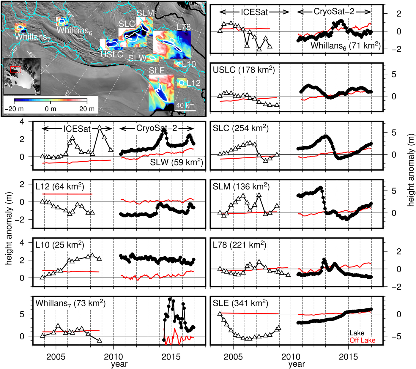
Fig. 2. Subglacial lakes of Mercer and Whillans ice streams. Map shows MODIS visual imagery (Scambos and others, Reference Scambos, Haran, Fahnestock, Painter and Bohlander2007) and the DEM for each lake region with the mean elevation for the region removed. Cyan lines are subglacial water flow paths based on Bedmap2 (Fretwell and others, Reference Fretwell2013) hydropotential gradients assuming uniform effective pressure and a standard sink-filling water routing algorithm (e.g. Le Brocq and others, Reference Le Brocq, Payne, Siegert and Alley2009); black line is the grounding line (Depoorter and others, Reference Depoorter2013). Inset shows location relative to ice velocity (Rignot and others, Reference Rignot, Mouginot and Scheuchl2011) using the same greyscale as Fig. 1. The extended time series of subglacial lake height anomaly corrected for regional height-changes is shown in black, while the regional height changes are shown in red. Triangles are derived from ICESat laser altimetry; circles are derived from CryoSat-2 radar altimetry.
Lake10 (25 km2), Lake12 (64 km2), Upper Subglacial Lake Conway (USLC; 178 km2), Whillans6 (71 km2), and Whillans7 (73 km2) were also sampled by CryoSat-2 SARIn mode. Ice-surface height over Lake10 increased by 2.5 m from late 2003 to early 2008. The surface height of the lake remained constant until the end of the CryoSat-2 period, but the region surrounding Lake10 increased in height by ~0.1 m a−1, resulting in a relative surface lowering across Lake10, after accounting for the regional trend.
At Lake12, surface height decreased by 1.4 m between the start of the mission in late 2003 and early 2006, increased by 1.1 m over the next 8 months, and decreased again by 1.0 m over the subsequent year. Surface height across Lake12 remained constant until late 2014 when it rapidly increased by 1.1 m over 4 months. The mean surface height over Lake12 slowly decreased back to the late 2014 level over the subsequent two years, at which point it increased again by 1.0 m over 4 months. Both of these rapid height-change events coincided with height-change events at SLW.
USLC is located on the southern shear margin of Whillans Ice Stream, and due to the rough ice surface, ICESat data were noisy. The overall trend for the ICESat period was surface lowering, with a total lowering signal of 2.5 m between mid 2004 and early 2008. During the CryoSat-2 period, height over USLC peaked in July 2011 at 4.5 m above the early 2008 low stand, and then decreased by 2.8 m over the subsequent 22 months. The cycle started again, with a 2.75-year period of increasing height (2.3 m) followed by surface lowering that continued to the end of the time series. During the CryoSat-2 period, four and a half years elapsed between successive peaks in surface height.
Further upstream, total height change at Whillans6 was −2.6 m between early 2004 and early 2008. During the CryoSat-2 period, height steadily increased from mid-2010 to mid-2013 at a rate of 0.23 m a−1. Between mid-2013 and the end of 2014, ice-surface height increased by 1.1 m over 2 months, were sustained at the anomalously high level for 8 months, and then decreased by 1.3 m over the next 7 months; the ice-surface height remained around this value from 2015 until the end of 2016. Whillans7 exhibited two periods of increasing height followed by decreasing height with an amplitude of 1–2 m during the ICESat mission. Situated at the edge of the SARIn-mode region after the mode mask was altered in 2014, this lake had sparse CryoSat-2 data, resulting in a time series of mostly noise during the CryoSat-2 period.
Kamb Ice Stream lakes
We analyzed three subglacial lakes on lower Kamb Ice Stream: KT1 (43 km2), KT2 (32 km2), and KT3 (39 km2) (Fig. 3). KT1 is at the same location as KambTrunk1 from Smith and others (Reference Smith, Joughin, Tulaczyk and Fricker2012), but its outline was refined by Kim and others (Reference Kim, Lee, Seo, Lee and Scambos2016). KT2 and KT2 were discovered by Kim and others (Reference Kim, Lee, Seo, Lee and Scambos2016), who derived activity time series with CryoSat-2 data, but did not assess any of the three regions during the ICESat period. Our results show that KT1 was the only lake of the three to exhibit dynamic behavior between 2003 and 2009, with height on the lake decreasing by 0.23 m a−1 after accounting for the 0.10 m a−1 regional thickening signal. All three lakes showed dynamic height changes during 2014, consistent with Kim and others (Reference Kim, Lee, Seo, Lee and Scambos2016). The height changes on these lakes were abrupt: ice-surface height at KT1 and KT3 increased by 2.5 m and 1.7 m over 4 months, while the mean height of KT2 increased by 1.7 m in a single month (equivalent to >20 m a−1). All three lakes exhibited different behavior after rapid height increases: KT1 remained elevated until the end of 2016, KT2's height decreased back to its pre-high-stand height over the subsequent 2.5 years, and KT3 returned to its pre-high-stand height in only 2 months.
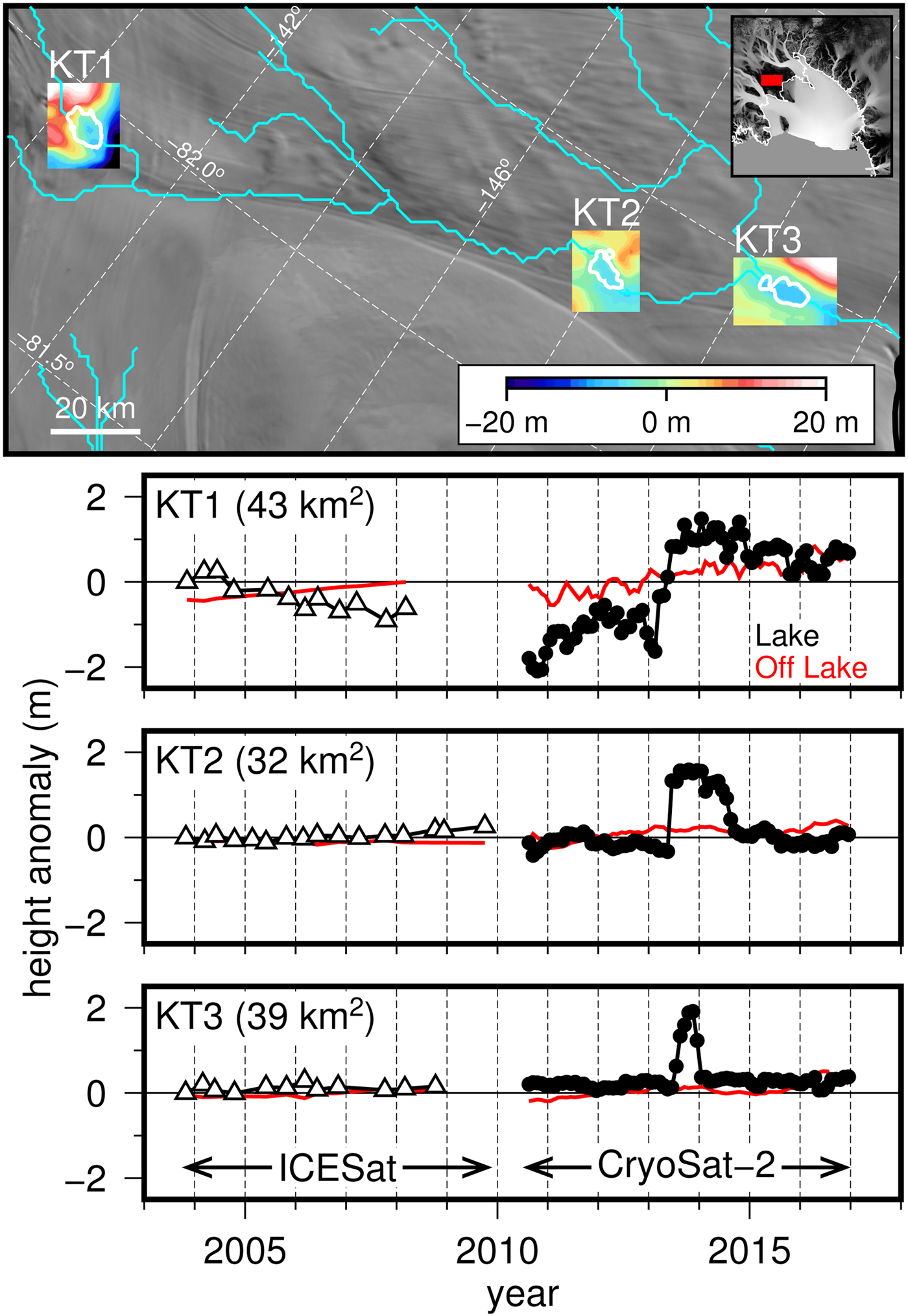
Fig. 3. Lower Kamb Ice Stream subglacial lakes map and extended time series. See caption of Fig. 2 for data sources.
MacAyeal Ice Stream lakes
During the ICESat period, the lakes beneath lower MacAyeal Ice Stream all exhibited periods of rapid height change separated by longer intervals of no change (Fig. 4), which is consistent with previous work (Fricker and others, Reference Fricker2010; Carter and others, Reference Carter2011). Mac1 (150 km2) underwent a height decrease in early 2004 (−5.8 m) and a height increase in mid-2007 (4.5 m). Mac2 (140 km2) only experienced one rapid height change event, with height increasing by 1.4 m over 3 months in 2005. For Mac2, we show mean lake height anomaly both corrected for the regional trend (Fig. 4, black line) and uncorrected for the regional trend (Fig. 4, blue line) as this lake is located a steep-walled surface depression, and the strong regional thinning trend (Fig. 4, red line) may represent dynamics of the (topographically) high regions rather than the low regions. Due to the long and narrow geometry of Mac3 (144 km2), ICESat observations were more limited here, but it appeared to undergo surface-height drawdowns in early 2004 (−1.4 m), early 2006 (−2.4 m) and late 2007/early 2008 (−2.0 m) and a 4 m increase in height in mid-2007.
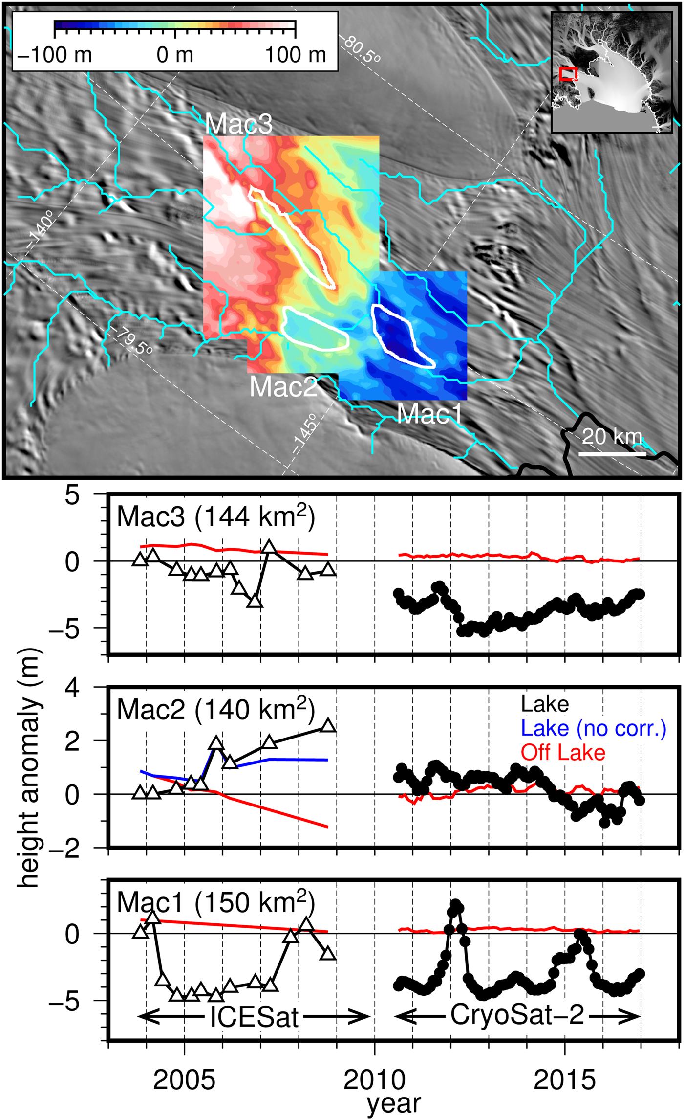
Fig. 4. Lower MacAyeal Ice Stream subglacial lakes map and extended time series. ‘Lake (no corr.)’ indicates the height anomaly on the lake not corrected for regional height-change. See caption of Fig. 2 for data sources.
Analysis of CryoSat-2 data over MacAyeal lakes revealed rapid switches from increasing height to decreasing height, demonstrating the value of this mission's increased temporal resolution. The surface height at Mac3 increased by 1.6 m over 6 months during 2011, sharply followed by a 3.4 m height decrease over 7 months. After this period, height increased by 0.50 m a−1 over the final 5 years of the time series. The surface lowering in late 2011 and early 2012 at Mac3 coincides with a large surface height anomaly at Mac1, located downstream. Here, surface height increased by 6.4 m over 9 months, then decreased to the pre-event height over the following 8 months. There appeared to be similar events, though smaller, which peaked in late 2013 (amplitude of 1–1.5 m) and early 2015 (amplitude of 4.2 m). Mac2, for which the time series is noisier during the CryoSat-2 period, generally experienced decreasing surface heights during 2014 (−1.7 m over 13 months) and also experienced a rapid height increase (1.2 m) in early 2016.
Institute Ice Stream lakes
InstituteE1 (441 km2) and InstituteW1 (81 km2) displayed similar activity during the ICESat period from late 2003 until 2008, both steadily increasing in height (InstituteE1 at 0.27 m a−1; InstituteW1 at 0.12 m a−1; Fig. 5). During 2008, surface height at InstituteE1 decreased by 2.2 m over 9 months, while surface height at InstituteW1 increased by 0.8 m. These two lakes were not covered by SARIn mode until mid-2013, when the mask was adjusted, resulting in a five-year gap between the ICESat and CryoSat-2 time series. Since this time, InstituteE1 showed minimal height variability, with the surface height at approximately the same level as at the end of the ICESat mission. The time series at InstituteW1 suggests a minor surface lowering over the lake until early 2014, followed by increasing surface height until the beginning of 2016, but the data over the small lake were sparse and the amplitude of the signal is small (<1 m).
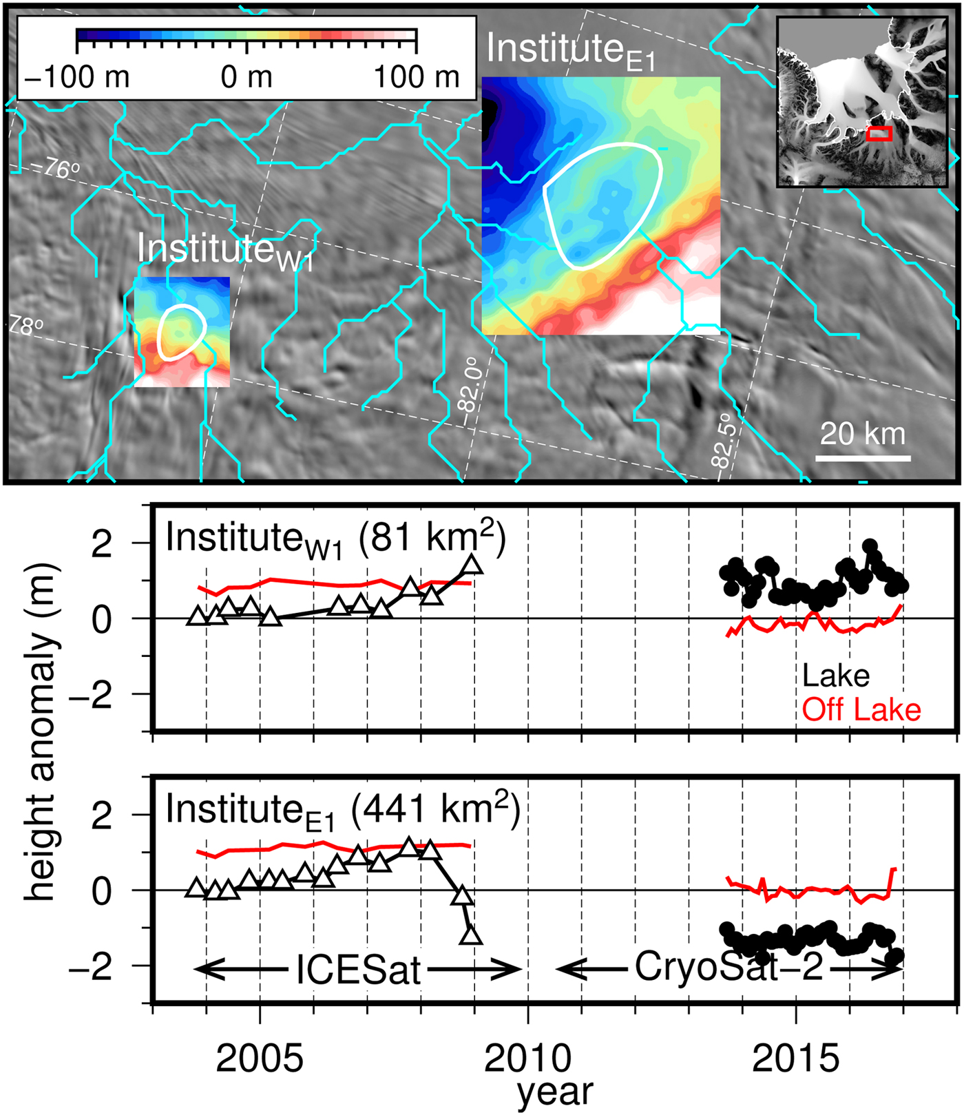
Fig. 5. Lower Institute Ice Stream subglacial lakes map and extended time series. See caption of Fig. 2 for data sources.
Other West Antarctic lakes
Five other lakes in West Antarctica were covered by CryoSat-2 SARIn-mode altimetry: Rutford1 (111 km2) near the grounding line of Rutford Ice Stream, and four lakes on upper Thwaites Glaicer – Thw70 (354 km2), Thw124 (561 km2), Thw142 (156 km2), and Thw170 (189 km2). During the ICESat period, only one ICESat track crossed Rutford1 with multiple repeats, causing our method to fail to produce a time series. As this lake is adjacent to the Ellsworth Mountains to the south, the rough terrain resulted in large uncertainties in the CryoSat-2 data both on and off the lake, failing to produce a time series during the CryoSat-2 period as well.
Time series derived from CryoSat-2 data for the Thwaites lakes during the the period 2010–16 were recently published by Smith and others (Reference Smith, Gourmelen, Huth and Joughin2017); these lakes were not previously analyzed with ICESat data. Because of the low temporal resolution of ICESat (2–3 campaigns per year) coupled with rough terrain in a frequently cloudy area, ICESat data for the Thwaites lakes were sparse: only two ICESat tracks crossed Thw70, which failed to produce a time series with our method due to a lack of coincident observations on both tracks; Thw124 underwent a surface lowering of 0.38 m a−1 through the ICESat period; Thw142 underwent two 2 m surface draw downs (in early 2005 and early 2007), but both only persisted for a single campaign, making it difficult to determine if these events were a real signal, a processing artifact, or noise; and the height of Thw170 steadily increased by a total of 1.7 m from early 2005 to mid-2006, followed by a decrease of 1.1 m until 2009, which were small amplitude signals compared with the 3.3 m decrease over 7 months in 2013 as observed by CryoSat-2 (Smith and others, Reference Smith, Gourmelen, Huth and Joughin2017).
East Antarctic subglacial lakes
LennoxKing1
LennoxKing1 is a small lake (35 km2) in the upstream catchment of the Lennox–King Glacier (Fig. 6). During the ICESat period, the surface height of this lake decreased by 0.9 m over 3.4 years (late 2004 to early 2008), followed by a surface-height increase of 0.4 m over the subsequent 9 months. During the CryoSat-2 period, there were small (<0.5 m), in-phase height fluctuations both on and off the lake, with no clear trend.
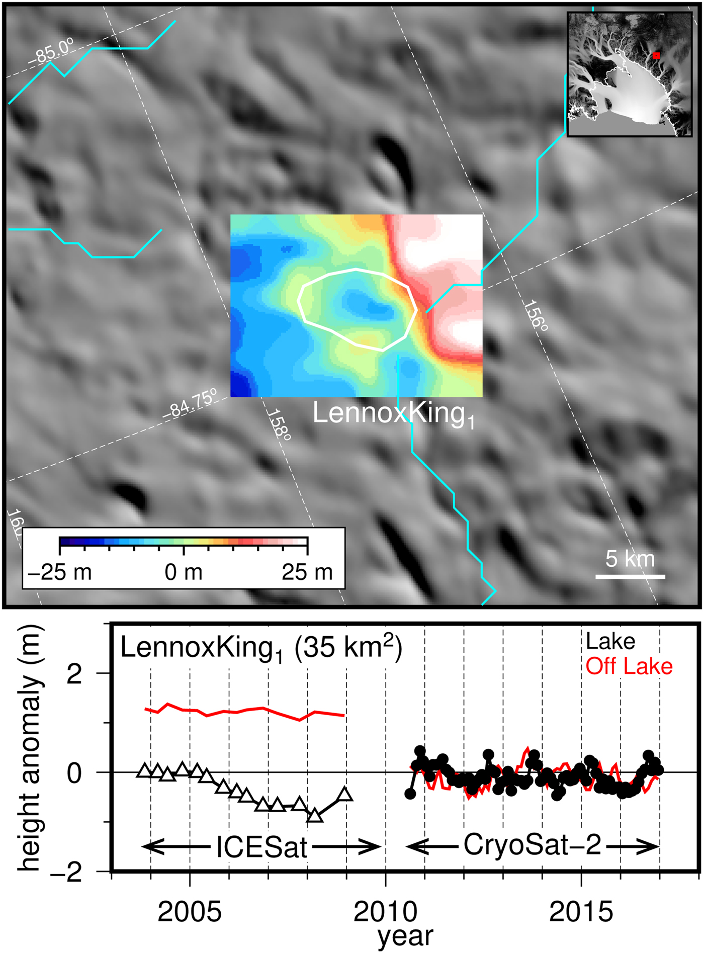
Fig. 6. LennoxKing1 subglacial lake map and extended time series. See the caption of Fig. 2 for data sources.
Cook West lakes
There are two lakes in the western catchment of Cook Ice Shelf, East Antarctica: CookW1 (190 km2; named Ninnis1 in Smith and others (2012); lake named Ninnis1 in Smith and others (Reference Smith, Fricker, Joughin and Tulaczyk2009) was renamed to Mertz1 in Smith and others (Reference Smith, Joughin, Tulaczyk and Fricker2012)) and CookW2 (227 km2; named Ninnis2 in Smith and others (Reference Smith, Fricker, Joughin and Tulaczyk2012)). The surface height decreased by 1.1 m between late 2004 and late 2007 at CookW1 and by 0.5 m between 2003 and 2005 at CookW2, before increasing by 0.3 m over the next 3.6 years of the record (Fig. 7). During the CryoSat-2 period, there was a negative height trend both on and off the lake at CookW1, with the lake-averaged height decreasing at 0.23 m a−1 after correcting for the regional signal. At CookW2, height remained constant over the 6.5-year time period, both on and off the lake.
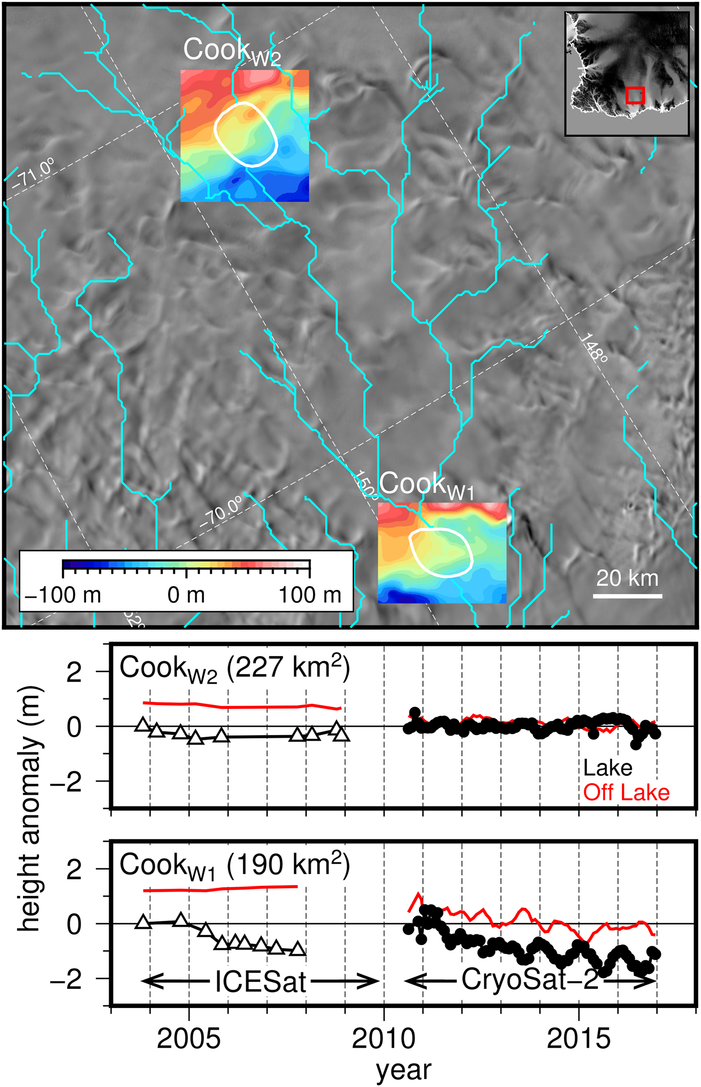
Fig. 7. Cook West subglacial lakes map and extended time series. See caption of Fig. 2 for data sources.
Slessor Glacier lakes
The Smith and others (Reference Smith, Joughin, Tulaczyk and Fricker2012) inventory reported five subglacial lakes on Slessor Glacier, three of which were covered by CryoSat-2 SARIn mode: Slessor1 (245 km2), Slessor2 (137 km2), and Slessor3 (107 km2) (Fig. 8). During the ICESat mission, ice-surface height at Slessor1 decreased from the start of the ICESat period (late 2003) to early 2006 at a rate of −0.33 m a−1 and then increased at 0.15 m a−1 until 2009. Slessor2 and Slessor3, which abut each other, exhibited changes of opposite sign during the ICESat period: height not corrected for regional changes at Slessor2 increased by 7.6 m, while height at Slessor3 decreased by 2.3 m.
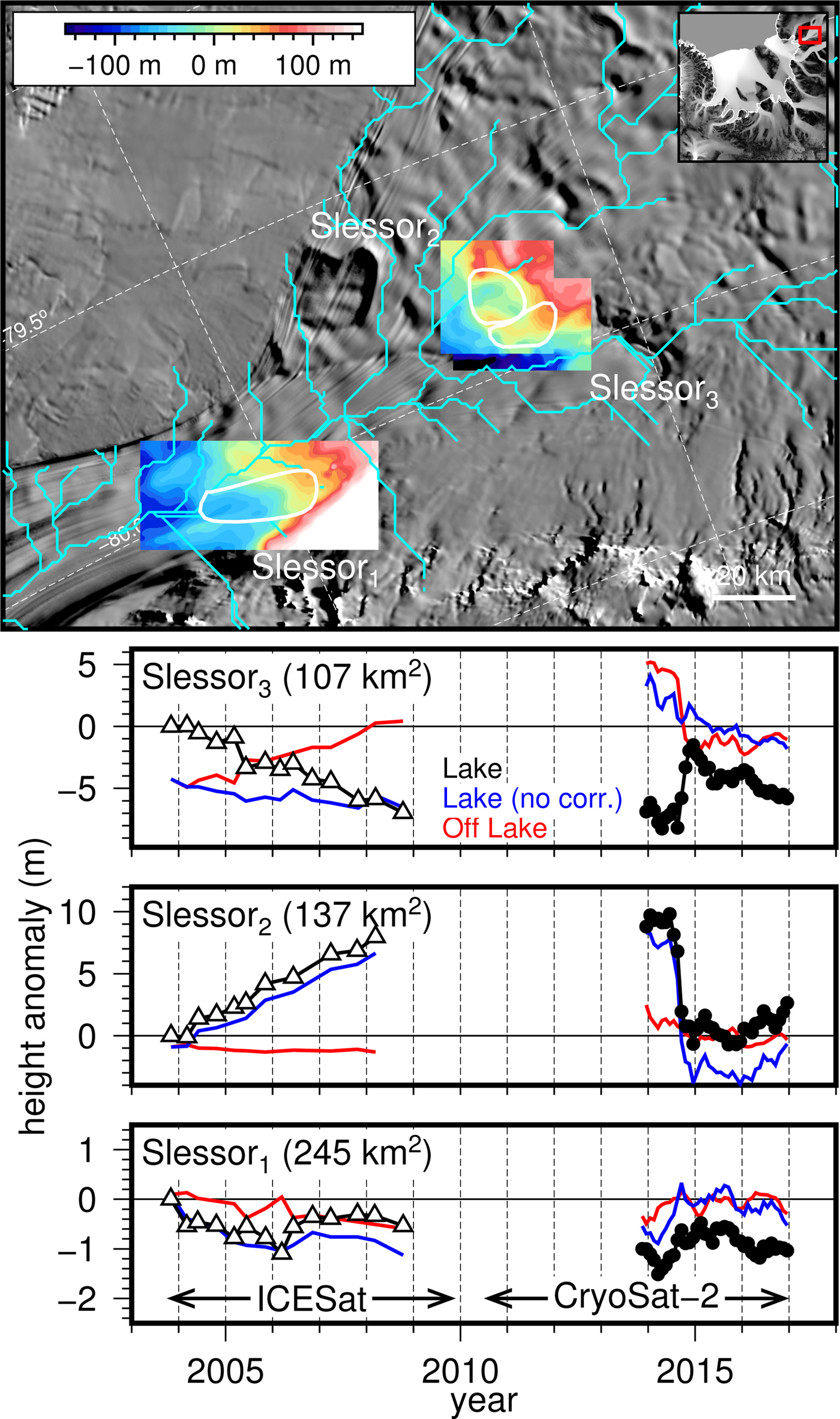
Fig. 8. Slessor Glacier subglacial lakes map and extended time series. ‘Lake (no corr.)’ indicates the height anomaly on the lake not corrected for regional height-change. See caption of Fig. 2 for data sources.
CryoSat-2 SARIn coverage only started in late 2013 for these lakes, providing just over 3 years of additional data. At the beginning of the 2013–2016 period, Slessor2 experienced a rapid height decrease of 10.5 m over 6 months. Because of this large dynamic signal in the region surrounding Slessor3, we could not apply the correction for regional ice dynamics. Data from within the boundary of Slessor3, however, showed a height-change signal that correlated with height changes at Slessor2, although smaller in magnitude. This correlated behavior contrasted with the anti-correlated behavior that occurred during the ICESat period. Data at Slessor1 were noisy with a large data gap in the middle of the lake due to CryoSat-2 SARIn mode preferentially sampling local high points, but there was no indication of a similarly large increase in surface height related to the decrease at Slessor2.
Totten Glacier lakes
Subglacial lakes Totten1 (567 km2) and Totten2 (711 km2) are both large subglacial lakes in the upstream catchment of Totten Glacier, East Antarctica (Fig. 9). From late 2003 to mid-2006, ice-surface height decreased by 1.9 m at Totten1, then increased by 1.3 m from 2006 to early 2009. Height at Totten2 decreased by 1.1 m between late 2004 and mid-2005, increased by 1.1 m over the next 1.8 years, and decreased again by 0.9 m until early 2008. During the CryoSat-2 mission, the surface height at Totten1 fell from the beginning of the CryoSat-2 period until mid-2011, hitting low stand near the same level as during the ICESat period. From this low stand, ice-surface height at Totten1 increased by 0.20 m a−1 until the end of the 2016. Totten2 experienced small height fluctuations, which appear to be in-phase with the regional fluctuations exhibited outside the lake boundaries. The regional time series is noisy due to Totten2's location at the edge of the SARIn-mode mask; we show the lake height-change time series before correcting for the regional trend (blue line) to highlight the minimal changes occurring within the boundary during the CryoSat-2 period.
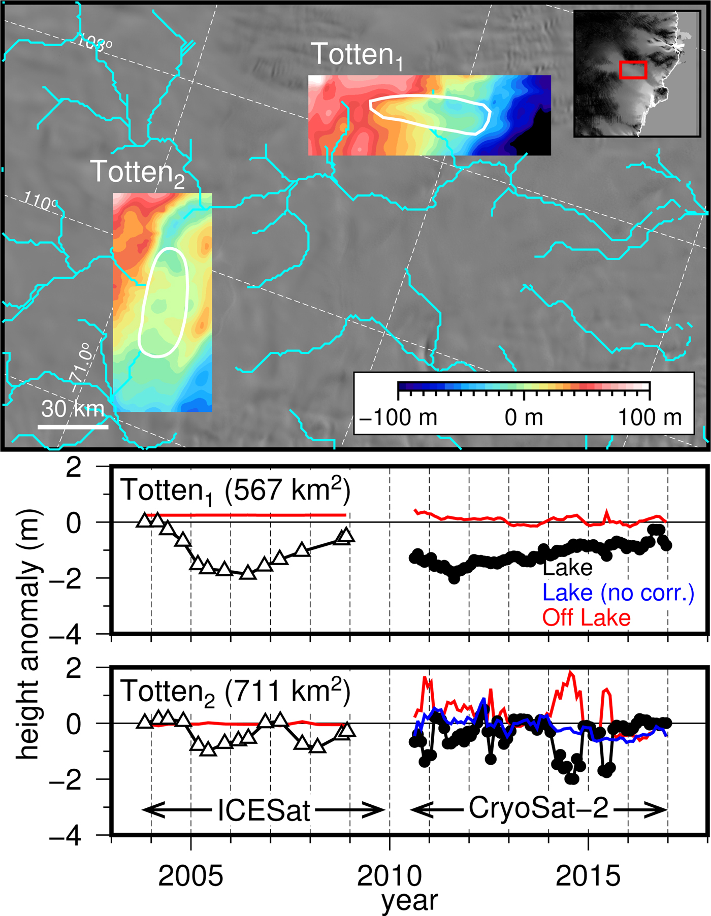
Fig. 9. Totten Glacier subglacial lakes map and extended time series. ‘Lake (no corr.)’ indicates the height anomaly on the lake not corrected for regional height-change. See caption of Fig. 2 for data sources.
Wilkes Land lakes
Wilkes1 (596 km2; Fig. 10) and Wilkes2 (179 km2) both increased in surface height throughout the duration of the ICESat mission (Wilkes1 by 0.5 m and Wilkes2 by 0.6 m). Wilkes1 did not undergo any height changes during the CryoSat-2 mission, remaining constant at 0.5 m above the height it was at the start of the ICESat period in 2003. The smaller Wilkes2 (not shown) experienced variable height changes during the CryoSat-2 period, which were in phase with regional changes.
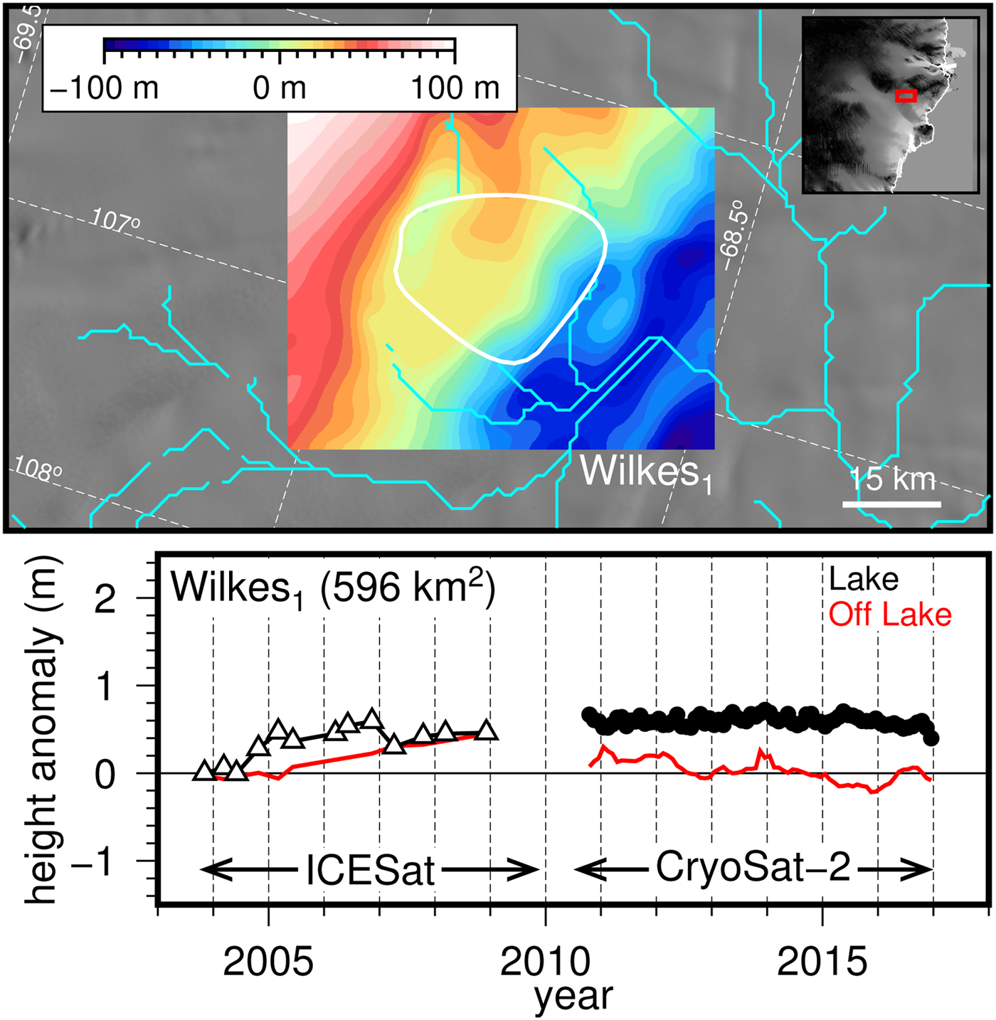
Fig. 10. Wilkes1 subglacial lake map and extended time series. See the caption of Fig. 2 for data sources.
Other East Antarctic lakes
Thirteen other active subglacial lakes in East Antarctica were sampled by CryoSat-2 SARIn mode. Many of these lakes (Byrds1, David1, Davids1, Lambert1) have rough surface topography, resulting in spatially biased sampling and noisy time series. CookE2 in the eastern catchment of Cook Ice Shelf, George V Land, was studied with CryoSat-2 by McMillan and others (Reference McMillan2013), who found a >60 m drawdown in the center of the lake and highlighted that SARIn-mode data tracks the rim of this lake's surface depression, with few observations within the depression itself. This issue with conventionally processed SARIn-mode data prevented us from generating a reliable time series for this lake. Surface height at CookE1 increased by 1.1 m between 2007 and 2008, coincient with the large drawdown of CookE2. Height slightly decreased through the 6.5-year CryoSat-2 period at a rate of −0.06 m a−1. The two Cook lakes were analyzed in detail by Flament and others (Reference Flament, Berthier and Rémy2014) with ICESat laser altimetry, Advanced Spaceborne Thermal Emission and Reflection Radiometer (ASTER) and Satellite Pour l'Observation de la Terre (SPOT) 5 stereo imagery, and Envisat radar altimetry.
CryoSat-2 mode-mask changes in 2013 extended the coverage to include lakes in the Filchner-Ronne Ice Shelf catchment, including Foundation1 and Foundation2 on lower Foundation Ice Stream and Rec1 and Rec2 on lower Recovery Ice Stream. A subsequent mode-mask change in 2016 provided observations over Foundation3, Foundation4, and Foundation5. Although there were an additional 1–3 years of CryoSat-2 data for these subglacial lakes, the data were noisy due to the rugged surface topography of Foundation Ice Stream; this prevented us from generating a reliable time series. The Recovery Ice Stream lakes were investigated by Fricker and others (Reference Fricker, Carter, Bell and Scambos2014). The additional CryoSat-2 data did not reveal any new height-change anomalies over Rec1, and data from Rec2 are limited as the CryoSat-2 mode-switch from SARIn to LRM occurred in the middle of the lake.
NEW INSIGHTS INTO ANTARCTIC SUBGLACIAL HYDROLOGY FROM EXTENDED TIME SERIES
The availability of CryoSat-2 SARIn-mode altimetry data since 2010 has allowed us to successfully generate a 13 year, combined laser-radar altimetry time series for 46 of the 132 active lakes in our new compiled inventory. We recorded large height-change events at 21 of these 46 subglacial lakes, which has provided new and important insights into Antarctica's subglacial hydrologic system that were not available through other means. In this discussion, we highlight three notable aspects of this system revealed by the new, extended active subglacial lake records: (i) the large event on Slessor Glacier, (ii) the inter-connected dynamics of MacAyeal Ice Stream, and (iii) insights into the spatial and temporal variability of active lakes.
(i) Slessor23 subglacial drainage, 2014
One of the main assumptions of our method is that the signal in the region surrounding any individual lake represents long-term, regional height change. In the case of Slessor Glacier, where two lakes abut one another, this assumption was violated; we therefore had to use alternate methods to investigate the large decrease in ice-surface height that occurs over Slessor2. Following the methods of Siegfried and others (Reference Siegfried, Fricker, Roberts, Scambos and Tulaczyk2014), we created a DEM-difference map before and after a surface-height anomaly. The resulting map of height differences (Fig. 11a) showed that the published outlines for both Slessor2 and Slessor3 were slightly offset relative to the location of height changes in the 2014 event and that the two lakes were likely a single larger lake. We traced the −5 m height-change contour to create a new outline for this combined height-anomaly (which we name Slessor23) and reprocessed the ICESat and CryoSat-2 data using the method we have developed in this work to generate a time series of height anomalies with this new outline (Fig. 11b).
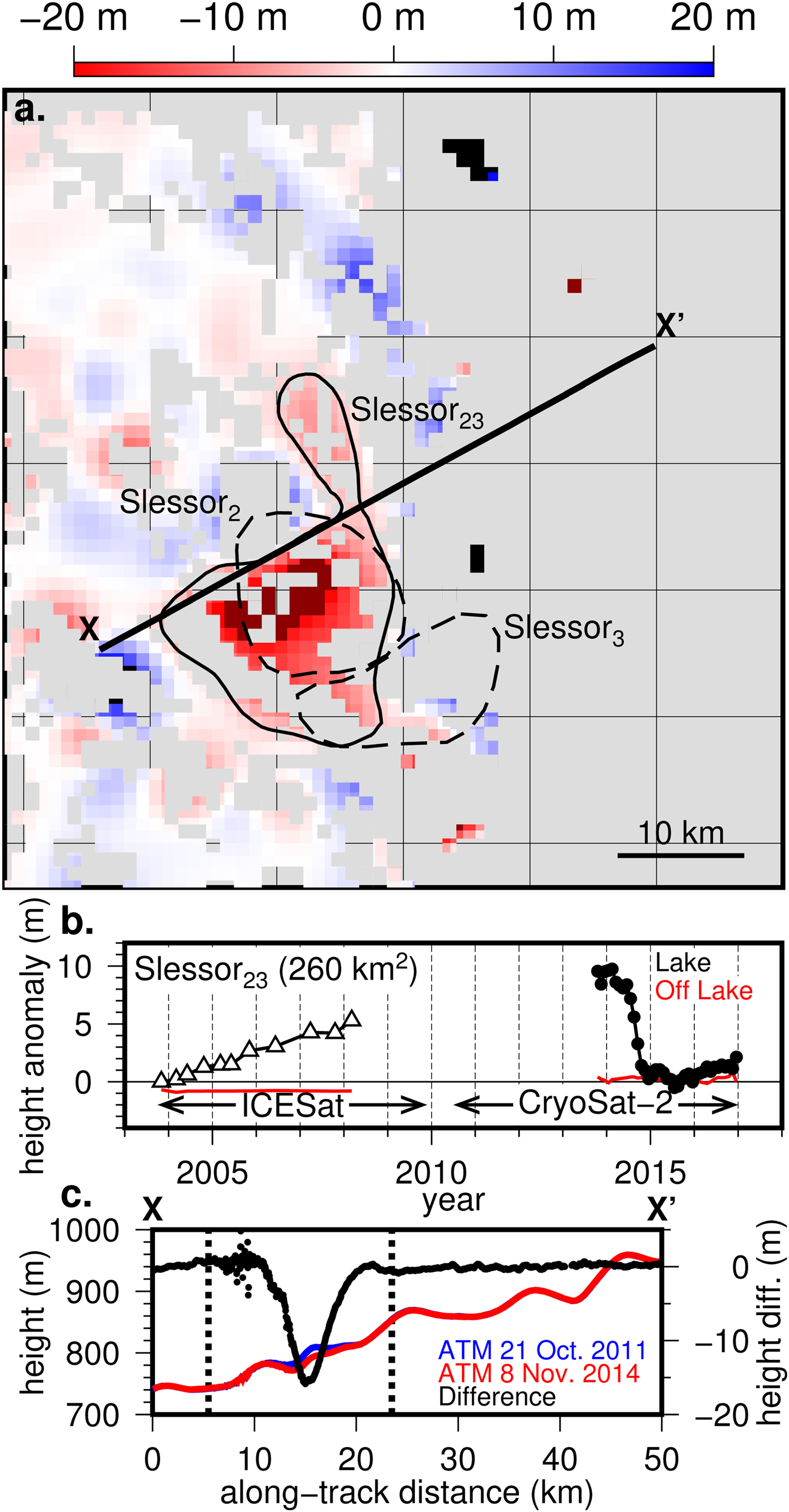
Fig. 11. Reanalysis of Slessor Glacier's height anomalies. (a) Relative height change (in meters) between Dec. 2013–Mar. 2014 and Nov. 2014–Feb. 2015 at Slessor2 and Slessor3, masked to show only locations that had CryoSat-2 observations during both periods. The region corresponding to the large subsidence (solid) is offset from the published lake outlines (dashed; Smith and others, Reference Smith, Joughin, Tulaczyk and Fricker2012). Profile X–X' is a repeat Operation IceBridge flight line, shown in (c). (b) Height-change time series for the new lake outline with the average lake height accounting for regional changes in black and the regional height change shown in red. (c) Nadir heights from ATM laser altimetry on 21 Oct. 2011 and 8 Nov. 2014 along the X–X' profile in (a) and the height difference between the two surveys with the limits of the lake marked by vertical dotted lines, which confirms both the location and magnitude large amplitude surface height anomaly seen in CryoSat-2 observations.
The newly defined lake had an area of 260 km2 and showed an average height change of −9.5 m over 10 months, with a peak 1-month height-change of −2.3 m (equivalent to −27.6 m a−1). We confirmed this anomaly using 2011 and 2014 laser altimetry surveys of Slessor Glacier by NASA Operation IceBridge's Airborne Thematic Mapper (Studinger, Reference Studinger2014), which showed a peak height anomaly of >15 m (Fig. 11c). Combining these lakes into a single lake resulted in our inventory of active subglacial lake boundaries containing 131 features, of which 45 were sampled by CryoSat-2 SARIn mode and 20 demonstrated anomalous height changes between 2008 and 2016.
The anomaly at Slessor23 represents one of the largest observed over all of Antarctica, with over 2.5 km3 of ice displaced over 10 months and 75% of this displacement occurring over a four-month period. The peak rate of ice displacement (−227 m3s−1) exceeds that of the largest subglacial lake drainage event in the inventory at CookE2 (McMillan and others, Reference McMillan2013) by over 40%. The mean rate of volume-change is over 30% larger at Slessor23 (−94 m3s−1) than the peak rate of change of the subglacial lake discharge event at Byrd Glacier, which caused a velocity increase of 10% (Stearns and others, Reference Stearns, Smith and Hamilton2008). Further analysis is needed to understand the dynamics of this large surface-height anomaly, including the underlying cause of anti-correlated height-changes during the ICESat period.
(ii) Connected hydrology on MacAyeal Ice Stream
On MacAyeal Ice Stream, the infrequent sampling by ICESat had prevented us from determining the exact timing of lake activity for the period 2003–09, reducing the ability to identify hydrological connections (Fricker and others, Reference Fricker2010). Our CryoSat-2 analysis revealed a clearer picture of the connectivity between subglacial lakes. The coincident timing between the peak rate of height decrease at Mac3 and the peak height at Mac1 suggests that these two features may be hydrologically linked, with water draining directly from Mac3 into Mac1, bypassing Mac2. This relationship between the displacement rates and height is similar to that inferred through GPS observations of surface heights farther south on the Siple Coast at the Mercer and Whillans ice streams (Siegfried and others, Reference Siegfried, Fricker, Carter and Tulaczyk2016). Moreover, the increased spatial resolution of CryoSat-2 DEMs in the area show a clear path of low hydropotential (i.e. lower elevation given relatively flat basal slopes) for subglacial water drainage from Mac3 to Mac1 (Fig. 4), which represents a different water flow route than that which would be predicted from Bedmap2 (Fretwell and others, Reference Fretwell2013). In future work, these DEMs could be evolved through time with more sophisticated models of subglacial water transport to better understand the connected hydrology and the potential for water route switching (e.g. Carter and others, Reference Carter, Fricker and Siegfried2013), especially in the context of other geophysical observations suggesting dynamic subglacial hydrology (Winberry and others, Reference Winberry, Anandakrishnan and Alley2009).
(iii) Spatial and temporal variability of active lakes
The extended record of surface-height anomalies has demonstrated that several, but not all, locations identified as active subglacial lakes continued to be active after the end of the ICESat mission in 2009. On Whillans, Kamb, MacAyeal, Institute, Thwaites, and Slessor ice streams, there were eight locations that exhibited large (>1 m) surface-height anomalies afor the period 2010–16, in addition to the 12 events previously reported using CryoSat-2 data (McMillan and others, Reference McMillan2013; Siegfried and others, Reference Siegfried, Fricker, Roberts, Scambos and Tulaczyk2014, Reference Siegfried, Fricker, Carter and Tulaczyk2016; Kim and others, Reference Kim, Lee, Seo, Lee and Scambos2016; Smith and others, Reference Smith, Gourmelen, Huth and Joughin2017). Following existing literature (e.g. Fricker and others, Reference Fricker, Scambos, Bindschadler and Padman2007; Smith and others, Reference Smith, Fricker, Joughin and Tulaczyk2009), we interpret these events as the surface expression of moving subglacial water.
For the Siple Coast (Mercer, Whillans, Kamb, and MayAyeal ice streams), active subglacial lakes appeared to be persistent features, as the same locations continued to experience dynamic height changes through the duration of the 13-year time series with fill/drain cycles ranging generally between 1 and 5 years. The event at Slessor23 likely took over a decade to evolve, consistent with three large, previously documented events at SLE (Fricker and others, Reference Fricker, Scambos, Bindschadler and Padman2007), CookE2 (McMillan and others, Reference McMillan2013), and Thw124 (Smith and others, Reference Smith, Gourmelen, Huth and Joughin2017). The distribution of subglacial lakes that are active across this continuum of timescales, but especially those with long-period height changes, remains unknown. These events highlight the need to develop methods for identifying active subglacial lake locations using datasets collected before and after the ICESat mission: our inventory only includes lakes that exhibited change during short time periods (years) relative to the long timescales of ice-sheet variability (decades to centuries).
Some of the subglacial lakes that continued to show dynamic behavior exhibited significant activity punctuated by periods of quiescence (e.g. SLW, L78, Mac1, KT1, and CookE1). These lakes are characterized by similar rates of surface rising and lowering with no extended period of high stand, which is distinct from other lakes in their regional hydrological systems that are characterized long periods of low-magnitude rates of increasing height followed by short, rapid period of surface lowering (e.g. SLM, CookE2). Other lakes in Antarctica appear to inflate and slowly deflate (e.g. L12, KT2). This implies that care must be taken when analyzing any single location: while some subglacial lakes may in fact impound and episodically release water, potentially driving variability in the basal hydrological system, others may passively react to changing basal conditions, potentially throttling the flow of subglacial water downstream. The regional hydrological context is required to understand any individual lake's impact on the larger ice-sheet system.
There is now evidence of large multiple-km3 vertical displacements of surface ice occurring under ice streams across Antarctica: on the Siple Coast (Fricker and Scambos, Reference Fricker and Scambos2009), in the Amundsen Sea Embayment (Smith and others, Reference Smith, Gourmelen, Huth and Joughin2017), on an outlet glacier in the Trans-Antarctic Mountains (Stearns and others, Reference Stearns, Smith and Hamilton2008), in George V Land (McMillan and others, Reference McMillan2013), and now in the eastern Filchner Ice Shelf catchment (Slessor Glacier, this study). These events appear to be widespread, but with only one drainage event captured for each of these four large lakes, it is not possible to determine whether these features will repeat with similar dynamics, or whether such events occur as infrequently as once per glacial cycle. Without additional context, the role of these features in Antarctic ice stream dynamics remains elusive: are these lakes impounding large quantities of subglacial water for decades, with episodic releases that could have long-term impacts on flow, or are the large, rapid height-change anomalies a form of noise within these systems as ice flows over a heterogenous bed?
Many locations identified as active subglacial lakes in the Smith and others (Reference Smith, Joughin, Tulaczyk and Fricker2012) inventory did not exhibit any dynamic behavior between 2010 and the end of 2016. In multiple cases, including on Totten Glacier, in Wilkes Land, and Institute Ice Stream, ICESat had observed small (<1 m) anomalies over large areas (resulting in relatively large volume changes given the low signal-to-noise ratio). This type of lake with fluctuations of tens of cm in surface height during the ICESat mission may be related to basal water features as has been assumed, but also may be related to variability in surface processes, variability in the stress regime, or even noise in the original ICESat data. In some cases, including at Whillans Ice Stream in West Antarctica and David, Totten, and Lennox King glaciers and in the western catchment of Cook Ice Shelf in East Antarctica, CryoSat-2 data, which has higher spatial resolution than ICESat (Siegfried and others, Reference Siegfried, Fricker, Roberts, Scambos and Tulaczyk2014), revealed that the observed small-magnitude height-anomalies on these lakes were in-phase with small height-anomalies in the region outside the lake boundaries. This correlation suggests that these areas reflect regional-scale changes rather than local hydrology. In these areas that were interpreted as lakes based on low-amplitude height-change signals, the original height-change time series must be reassessed as more data become available in order to develop sound interpretations of the underlying glaciological processes.
Finally, many subglacial lakes we investigated, especially those in East Antarctica, were located in areas of steep or rough surface topography, which significantly impacts the effectiveness of conventional CryoSat-2 SARIn-mode altimetry. Previous work has established that, in areas of steep terrain, the SARIn-mode waveform can be unwrapped yielding a swath of height data instead of an individual footprint (e.g. Hawley and others, Reference Hawley, Shepherd, Cullen, Helm and Wingham2009; Gray and others, Reference Gray2013; Smith and others, Reference Smith, Gourmelen, Huth and Joughin2017). Applying swath mapping to this subset of lakes, similar to Smith and others (Reference Smith, Gourmelen, Huth and Joughin2017), will likely provide a more precise time series of subglacial lake activity during the CryoSat-2 period, and future work investigating dynamic hydrology in these individual catchments should revisit these lakes considering SARIn-mode phase data.
SUMMARY
We have used ICESat laser altimetry and CryoSat-2 radar altimetry to produce records of surface-height change from 2003 to 2016 for 46 active subglacial lakes in Antarctica, extending existing time series by 8 years. We found that two previously documented lakes were more likely one single lake (reducing the total to 45), and that 20 lakes experienced significant height-changes between 2008 and 2016. One of these events was located on Slessor Glacier and had one of the highest rate of volume displacement ever recorded in Antarctica, peaking at over 220 m3s−1. Our study has also shown that some of these features may not be the result of dynamic subglacial hydrology, suggesting that our mapping and understanding of active subglacial lakes, a part of the basal water system only discovered in the last decade, are still immature. Our final inventory contains 131 active subglacial lake locations across Antarctica.
Ice-sheet models that predict the future state of Antarctica, and its contribution to global sea-level change, require accurate representation of evolving basal conditions. The basal environment is challenging to observe and active subglacial lakes provide one window into dynamic basal processes that can be routinely monitored on the continent scale. While extending the record of a subset of active subglacial lakes is a first step, our existing knowledge of active lakes remains limited by the short duration and limited spatial coverage of altimeter missions used to monitor them. Future polar altimetry missions, with more advanced instrumentation (e.g. ICESat-2, scheduled for launch in 2018) will provide new insights into the dynamic ice-bed interface. To maximize the scientific value of these new altimetry datasets, we also need rigorous cross–calibration experiments in Antarctica to ensure continuity of our surface-height change time series between missions.
ACKNOWLEDGMENTS
We thank the National Snow and Ice Data Center, NASA, and the European Space Agency for data access; NASA (grants NNX11AQ78H and NNX17AI03G), NSF (grants 0838885 and 1543441), and the George Thompson Postdoctoral Fellowship for funding; Ben Smith, Choon Ki Lee, and Malcolm McMillan for new subglacial lake outlines; Brent Minchew and two anonymous reviewers for comments that improved the manuscript; and Sasha P. Carter for years of fruitful discussion about dynamic subglacial hydrology. Our inventory of subglacial lake outlines and corresponding height-change time series will be available at NSIDC.


 Open access