The collection of MATLAB statements and screen display:
>> x = [1 2 3 4 5 6 7 8 9 10]
x =
1 2 3 4 5 6 7 8 9 10
>> x = [1 2 3 4 5 6 7 8 9 10]; %Note
how the display of result is suppressed
>> x = x'
x =
1
2
3
4
5
6
7
8
9
10
>> x = 1:1:10
x =
1 2 3 4 5 6 7 8 9 10
>> y = 0:0.1:20;
>> size(y)
ans =
1 201
>> a = [1 2 3 ; 4 5 6 ; 7 8 9] %To create a matrix
a =
1 2
3
4 5
6
7 8
9
>> p1=[1 -5 4] %The section on defining and multiplying polynomials
p1 =
1 -5 4
>> p2=[1 0 4]
p2 =
1 0 4
>> p3=[1 -5 0]
p3 =
1 -5 0
>> p4=[1 3];
>> conv(p1,p4)
ans =
1 -2 -11 12
>> conv([1 -5 4],[1 3])
ans =
1 -2 -11 12
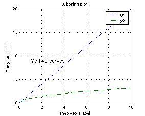
>> y1 = 2*x
y1 =
2 4 6 8 10 12 14 16 18 20
>> y2 = sqrt(x)
y2 =
Columns 1 through 7
1.0000 1.4142 1.7321 2.0000 2.2361 2.4495 2.6458
Columns 8 through 10
2.8284 3.0000 3.1623
>> b = sqrt(a) %Further demonstration of array operation using
>>
%the matrix "a" created earlier
b =
1.0000 1.4142 1.7321
2.0000 2.2361
2.4495
2.6458 2.8284
3.0000
>> y3 = y1 + y2
y3 =
Columns 1 through 7
3.0000 5.4142 7.7321 10.0000 12.2361 14.4495 16.6458
Columns 8 through 10
18.8284 21.0000 23.1623
>> c = a*b
c =
12.9373 14.3716 15.6310
29.8745 33.8078 37.1757
46.8118 53.2439 58.7203
>> d = a.^3
d =
1 8
27
64 125 216
343 512 729
>> a3 = a^3
a3 =
468
576 684
1062
1305 1548
1656
2034 2412
>> e = a.*b
e =
1.0000 2.8284 5.1962
8.0000 11.1803 14.6969
18.5203 22.6274 27.0000
| Note: |
| Please do not be alarmed by the "\" operator; it is just MATLAB's special way to say "solve Ax=b." Like the 3D plots below, it is just an illustration of features available in MATLAB and not what we'll need in later chapters. (We'll clear this up in future editions of the text.) |
>> A = [ 4 -2 -10; 2 10 -12; -4 -6 16];
>> b = [-10; 32; -16];
>> x = A\b
x =
2.0000
4.0000
1.0000
>> C = inv(A);
>> x = C*b
x =
2.0000
4.0000
1.0000
>> %You'd only know what LU decomposition
means if you have taken
>> %a course on numerical methods.
Quickly, it is a method to solve
>> %a linear system of equations.
>> [L,U] = lu(A);
>> x = inv(U)*inv (L)*b
x =
2.0000
4.0000
1.0000
>> [X,D] = eig(A)
X =
0.9317 -0.2882 -0.7844
0.1902 -0.6621 0.6174
0.3095 0.6918
0.0586
D =
0.2703
0 0
0 23.4088
0
0
0 6.3208
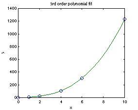
>> x = [ 0 1 2 4 6 10]; %The demonstration
of polynomial fitting
>> y = [ 1 7 23 109 307 1231];
>> c = polyfit(x,y,3)
c =
1.0000 2.0000 3.0000 1.0000
>> xfit=1:0.5:10;
>> yfit=xfit.^3 + 2*xfit.^2 + 3*xfit +1;
>> plot(x,y,'o', xfit,yfit)
>> title('3rd order polynomial fit')
>> xlabel('x'), ylabel('y')
>> % Optional reading from here on -- 3D plotting
for fun
>> % Don't worry about the functions that
we need to use in this segment.
>> % You won't see and use them
again. We just can't help but to
>> % show off some neat MATLAB plotting capabilities.
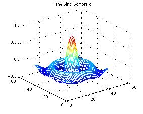
>> x= -10:0.5:10;
>> y=x';
>> x2=ones(size
(y))*x; %ones() generates an array containing all
"1"
>> y2=y*ones(size (x));
>> r=sqrt(x2.^2 + y2.^2) + eps; %The addition of "."
to the operators does
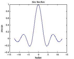
>> z=sin(r)./r; %element-by-element
operation to the arrays.
>> mesh(z)
>> title('The Sinc Sombrero')
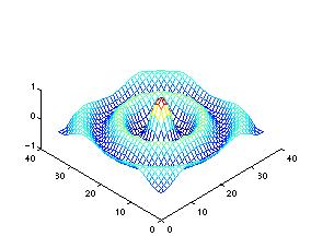
>> %A demonstration of Bessel function calculation
and plotting
>>
>> [x,y]=meshgrid(-12:.7:12, -12:.7:12);
%Generates a 2D array of points
>> r=sqrt(x.^2+y.^2);
>> z= bessel(0,r);
>> csc=[-45 60]; %Defines our own color
scaling vector for mesh()
>> mesh(z,csc)