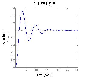
The collection of MATLAB statements and screen display:
>> %Step and impulse response simulations
>> q=1;
>> p=[1 0.4 1];
>> G=tf(q,p)
Transfer function:
1
---------------
s^2 + 0.4 s + 1
>> step(G)
>>%Try "help step" yourself
| New features in MATLAB 6 |
| If you click on a curve, the position is marked by a black square, and a small subwindow will pop out to report the coordinates. If you drag the small black square along the curve, the information in the subwindow will be updated instantaneously. |
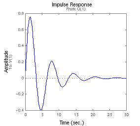
Zero/pole/gain:
2
--------------------
(s+2) (s^2 + 2s + 2)
>> step(G,H)
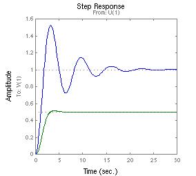
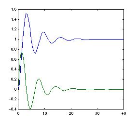
ans =
-0.2000 + 0.9798i
-0.2000 - 0.9798i
>> damp(G)
Eigenvalue Damping Freq. (rad/s)
-2.00e-01 + 9.80e-01i 2.00e-01
1.00e+00
-2.00e-01 - 9.80e-01i 2.00e-01
1.00e+00
>> %Now onto the section doing sinusoidal input
and response
>> q=[2 1];
>> p=conv([4 1],[1 1]);
>> G=tf(q,p)
Transfer function:
2 s + 1
---------------
4 s^2 + 5 s + 1
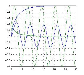
>> t=0:0.5:30;
>> u=sin(t);
>> y=lsim(G,u,t); %Will
calculate the sinusoidal response
>> plot(t,y,t,u,'-.'), grid
>> hold
Current plot held
>> ys=step(G,t);
>> yi=impulse(G,t);
>> plot(t,ys,t,yi)
>> hold off
q =
-1 10
p =
1 10
>> [q,p]=pade(0.2,2)
q =
1 -30 300
p =
1 30 300
Note: For the remindar of Session 3, you will have to try out
the LTI Viewer yourself. The section on Runge-Kutta integration is optional
because we don't really need it in this course. Same with the section on
importing and exporting data.