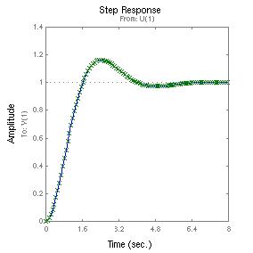
The collection of MATLAB statements and screen display:
>> %Example 4.1
>> z=0.5;
>> wn=1.5;
>> q=wn*wn;
>> p=[1 2*z*wn wn*wn]
p =
1.0000 1.5000 2.2500
>> roots(p)
ans =
-0.7500 + 1.2990i
-0.7500 - 1.2990i
>> [a,b,c,d]=tf2ss(q,p)
a =
-1.5000 -2.2500
1.0000
0
b =
1
0
c =
0
2.2500
d =
0
>> eig(a) %should be identical to the poles
ans =
-0.7500 + 1.2990i
-0.7500 - 1.2990i
>> [q2,p2]=ss2tf(a,b,c,d,1) %Should recover q(s) and p(s)
q2 =
0
0 2.2500
p2 =
1.0000 1.5000 2.2500
>> %Set up according to text
>> a=[0 1; -2.25 -1.5]; b=[0; 2.25]; c=[1 0]; d=0;
>> eig(a) %still
the same!
ans =
-0.7500 + 1.2990i
-0.7500 - 1.2990i
>> [qs,ps]=ss2tf(a,b,c,d,1)
qs =
0
0 2.2500
ps =
1.0000 1.5000 2.2500
>> %Repeat with the object-oriented state-space
models
>> q=2.25;
>> p=[1 1.5 2.25];
>> [a,b,c,d]=tf2ss(q,p);
>> sys_obj=ss(a,b,c,d)
a =
x1 x2
x1
-1.5 -2.25
x2
1 0
b =
u1
x1
1
x2
0
c =
x1 x2
y1
0 2.25
d =
u1
y1
0
Continuous-time model.
>> eig(sys_obj.a) %eigenvalue of state matrix a same as the poles
ans =
-0.7500 + 1.2990i
-0.7500 - 1.2990i
>> tf(sys_obj) %Get the transfer function back
Transfer function:
2.25
------------------
s^2 + 1.5 s + 2.25
>> %Starting from the transfer function
>> sys2=ss(tf(q,p))
a =
x1 x2
x1
-1.5 -1.125
x2
2 0
b =
u1
x1
1
x2
0
c =
x1 x2
y1
0 1.125
d =
u1
y1
0
Continuous-time model.
>> eig(sys2.a) %Another check
ans =
-0.7500 + 1.2990i
-0.7500 - 1.2990i
>> %The minor tidbits
>> printsys(a,b,c,d)
a =
x1 x2
x1
-1.50000 -2.25000
x2
1.00000
0
b =
u1
x1
1.00000
x2
0
c =
x1 x2
y1
0 2.25000
d =
u1
y1
0
>> printsys(q,p,'s')
num/den =
2.25
------------------
s^2 + 1.5 s + 2.25
>> [a,b,c,d]=ord2(wn,z) % good for only q=1
a =
0
1.0000
-2.2500 -1.5000
b =
0
1
c =
1 0
d =
0
>> %Time response simulation
>> %Try using LTI Viewer yourself
>> %We'll do Example 4.1 with plotting statements
here
>> a=[0 1; -2.25 -1.5]; b=[0; 2.25]; c=[1 0]; d=0;
>> sys=ss(a,b,c,d);
>> step(sys)
>> hold
Current plot held
>> G=tf(2.25,[1 1.5 2.25]);
>> step(G,'x')
>> hold off
>> %Transformations
>> %Example 4.6
>> A=[0 1 0; 0 -1 -2; 1 0 -10];
>> rank(A)
ans =
3
>> eig(A)
ans =
-0.2902
-0.6877
-10.0221
>> [P,L] = eig(A)
P =
0.9557 -0.8208 0.0216
-0.2773 0.5644 -0.2164
0.0984 -0.0881 -0.9761
L =
-0.2902
0 0
0 -0.6877
0
0
0 -10.0221
>> a = inv(P)*A*P %Check that we can really diagonalize the matrix
a =
-0.2902 -0.0000 -0.0000
0.0000 -0.6877 -0.0000
-0.0000 0.0000 -10.0221
>> % Second route
>> B=[0; 2; 0];
>> C=[1 0 0];
>> D=[0];
>> S=ss(A,B,C,D);
>> SD=canon(S)
a =
x1 x2
x3
x1
-0.29018
0 0
x2
0 -0.6877
0
x3
0 0
-10.022
b =
u1
x1
5.2524
x2
6.1155
x3
-0.022556
c =
x1 x2
x3
y1
0.95572 -0.82076
0.02159
d =
u1
y1
0
Continuous-time model.
>> %The 3rd alternative
>> SD=ss2ss(S,inv(P))
a = %Numerically, the
algorithm behind this method is not as clean
x1 x2
x3
x1
-0.29018 -1.6646e-16 -3.9409e-15
x2
1.1919e-16 -0.6877 -3.9643e-15
x3
-4.9829e-17 -2.5323e-17 -10.022
b =
u1
x1
5.2524
x2
6.1155
x3
-0.022556
c =
x1 x2
x3
y1
0.95572 -0.82076
0.02159
d =
u1
y1
0
Continuous-time model.
>> %Find the observable canonical form
>> SO=canon(S,'companion')
a =
x1 x2
x3
x1
0 0
-2
x2
1 0
-10
x3
0 1
-11
b =
u1
x1
1
x2
0
x3
0
c =
x1 x2
x3
y1
0 2
-2
d =
u1
y1
0
Continuous-time model.
>> roots([1 11 10 2]) % Check the results
ans =
-10.0221
-0.6877
-0.2902
>> poly(A)
ans =
1.0000 11.0000 10.0000
2.0000
>> %Optional reading, using Appendix of Chapter
4 to find the canonical forms ourselves
>> P=[B A*B A^2*B];
>> inv(P)*A*P
ans =
0 0
-2
1 0 -10
0 1 -11
>> inv(P)*B
ans =
1
0
0
>> poly(A); %just a check
>> M=[10 11 1; 11 1 0; 1 0 0];
>> T=P*M;
>> inv(T)*A*T
ans =
0
1.0000 0
0
0 1.0000
-2.0000 -10.0000 -11.0000
>> inv(T)*B
ans =
0
-0.0000
1.0000
>> %Onto Example 4.8
>> G=zpk([],[-1 -2 -3],1);
>> S=ss(G);
>> eig(S) %Check
ans =
-3
-2
-1
>> [P,L]=eig(S.a)
P =
1.0000 0.5774 -0.4082
0 -0.5774
0.4082
0
0.5774 -0.8165
L =
-3 0
0
0 -2
0
0 0
-1
>> inv(P)*S.a*P % Just a check of L
ans =
-3.0000
0 0
0 -2.0000
0
0
0 -1.0000
>> SD=canon(S) %find the diagonalized system
a =
x1 x2
x3
x1
-3 0
0
x2
0 -2
0
x3
0 0
-1
b =
u1
x1
0.5
x2
-1.7321
x3
-1.2247
c =
x1 x2
x3
y1
1 0.57735 -0.40825
d =
u1
y1
0
Continuous-time model.
>> inv(P)*S.b % Identical to SD.b
ans =
0.5000
-1.7321
-1.2247
>> S.c*P % Identical to SD.c
ans =
1.0000 0.5774 -0.4082
>> SO=canon(S,'companion') %observable canonical form
a =
x1 x2
x3
x1
0 0
-6
x2
1 0
-11
x3
0 1
-6
b =
u1
x1
1
x2
0
x3
0
c =
x1 x2
x3
y1
0 0
1
d =
u1
y1
0
Continuous-time model.