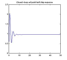
The collection of MATLAB statements and screen display:
>> %Make sure you have a chance to try out Simulink.
>> %You can start with using our sample files.
>> %Here, we'll begin with the section using
control toolbox functions.
>> %Step 1, the PI controller and process functions
>> km=2;
>> kc=10;
>> taui=100;
>> Gc=tf(km*kc*[taui 1], [taui 0])
Transfer function:
2000 s + 20
-----------
100 s
>> kp=1;
>> taup=5;
>> Gp=tf(kp, [taup 1])
Transfer function:
1
-------
5 s + 1
>> %Step 2, the feedback path function
>> taum=1;
>> Gm=tf(1, [taum 1])
Transfer function:
1
-----
s + 1
>> %Step 3, the closed-loop function
>> Gcl=feedback(Gc*Gp,Gm)
Transfer function:
2000 s^2 + 2020 s + 20
-------------------------------
500 s^3 + 600 s^2 + 2100 s + 20
>> %Step 4, check the closed-loop poles
>> pole(Gcl)
ans =
-0.5952 + 1.9581i
-0.5952 - 1.9581i
-0.0095
>> dcgain(Gcl) %With a PI controller, the closed-loop steady state gain should be unity
ans =
1
>> %step(Gcl) default plot is poorly scaled in
this problem.
>> %So we'll do the following to have a better
look:
>> [y,t]=step(Gcl);
>> plot(t,y)
>> axis([0 50 0 2.5])
%"zoom
in" closer
>> %Use our own derivations on a proportional
controller
>> kc=1;
>> kp=0.8;
>> taup=10;
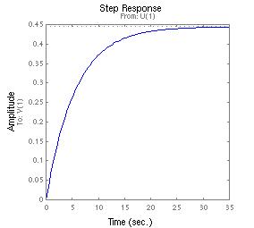
>> Gcl=tf(kc*kp, [taup 1+kc*kp])
Transfer function:
0.8
----------
10 s + 1.8
>> pole(Gcl)
ans =
-0.1800
>> step(Gcl);
ans =
-10.0221
-0.6877
-0.2902
>> G1=tf(1,[1 0]);
>> G2=tf(2,[1 1]);
>> H=tf(1,[1 10]);
>> Gcl=feedback(G1*G2,H);
>> pole(Gcl)
%check that the closed-loop poles are indeed correct
ans =
-10.0221
-0.6877
-0.2902
>> %The eigenvalues of the state-space representation
should be identical to the closed-loop poles
>> ssm=ss(Gcl);
>> eig(ssm.a)
ans =
-10.0221
-0.6877
-0.2902
>> tf(ssm) %We can go backward
Transfer function:
2 s + 20
-----------------------
s^3 + 11 s^2 + 10 s + 2
>> Gcl %Yes, it is the same Gcl as before
Transfer function:
2 s + 20
-----------------------
s^3 + 11 s^2 + 10 s + 2
>> %One final check. Should recover the same eigenvalues
and transfer function
>> a=[0 1 0; 0 -1 -2; 1 0 -10];
>> b=[0; 2; 0];
>> c=[1 0 0];
>> d=0;
>> eig(a)
ans =
-0.2902
-0.6877
-10.0221
>> [q3,p3]=ss2tf(a,b,c,d,1)
q3 =
0
0.0000 2.0000 20.0000
p3 =
1.0000 11.0000 10.0000
2.0000