Matlab Session 6 Results

MATLAB Session 6 Results

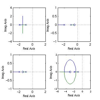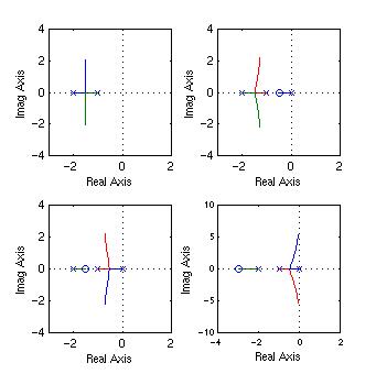
The collection of MATLAB statements and screen display:

>> %Root locus plots
>> p=[1 6 11 6];
>> roots(p)

ans =

   -3.0000
   -2.0000
   -1.0000

New feature in MATLAB 6

If you click right on a locus, the position is marked by a black square, and a small subwindow will pop out, reporting the gain, the pole coordinates, the damping ratio and percent overshoot of the chosen closed-loop pole. If you drag the small black square along the locus, the information in the subwindow will be updated instantaneously.

For all practical purposes, this new feature replaces the need of the sgrid() and rlocfind() functions.

>> G=tf(1,p);
>> rlocus(G)

>> %Adding an open-loop zero to cancel the open-loop pole at -1
>> G=tf([1 1],p);
>> rlocus(G)

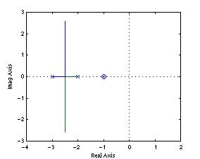
>> %Two more examples
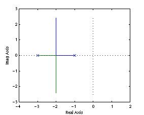
>> G=zpk([],[-1 -3],1) %Second order example

Zero/pole/gain:
1
-----------
(s+1) (s+3)

>> rlocus(G)

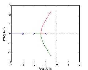
>> G=zpk([],[-1 -2 -3],1) %Third order example

Zero/pole/gain:
1
-----------------
(s+1) (s+2) (s+3)

>> rlocus(G)

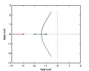
Note: This result is typical. The MATLAB default plot does not necessarily cross the imaginary axis. If you want to find the ultimate gain with rlocfind(), you will need to do the root locus plot with your own gain vector -- what will be illustrated below.

>> %The optional reading section
>> q=[2/3 1];
>> p=[1 6 11 6];
>> poles=roots(p)'

poles =

-3.0000 -2.0000 -1.0000

>> zeros=roots(q)'

zeros =

-1.5000

>> G=tf(q,p)

Transfer function:
0.6667 s + 1
----------------------
s^3 + 6 s^2 + 11 s + 6

>> %Defining our own gain vector. May take some trial-and-error
>> %to get good plotting results.
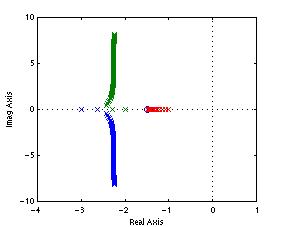
>> k=0:0.5:100;

>> rlocus(G,k);

>> %Alternate route of doing the plot that can be more instructive
>> %at the learning stage
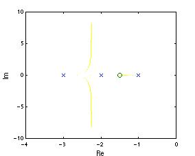
>> r=rlocus(G,k);
>> plot(r,'y.') %Deviation from text. Forcing all dots to be yellow here.
>> hold
Current plot held
>> py=[0 0 0];
>> qy=0;
>> ax=[0 0]; ay=[-4 4];
>> plot(poles,py,'x', zeros,qy,'o', ax,ay,'-')

>> %Another deviation from text. Using our own axis to better
>> %see the open-loop pole at -3.
>> axis([-4 0 -10 10]);

>> xlabel('Re'), ylabel('Im')
>> hold off

>> %Another alternative that will give the same result
>> plot(r,'y.')
>> hold
Current plot held
>> pzmap(G)

>> %Drawing damping ratio and natural frequency grid lines
>> rlocus(G)
>> sgrid(0.7,1)
>> %try rlocfind(G) yourself

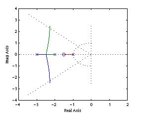
New feature in MATLAB 6

The sisotool has replaced the older rltool.

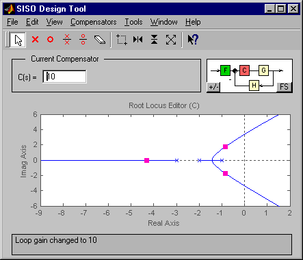
>> %Launching the SISO graphics design
>> %tool (with the root locus view)
>> sisotool(' rlocus')
>> %or if you know ahead of time the plant function to be used already
>> sisotool(' rlocus', G)

What you find is a really nicely desgined panel of tools. Its usage is pretty self-explanantory and point-and-click. When the sisotool is launched, it will ask if you would like to see Help. Say yes if this is the first time you use the tool or if you need on-line help. Here are some brief comments:

By default, the compensator C(s) is a proportional controller, and the root locus computation varies the value of this quantity "Gain" to draw the loci. If you click on the "Current Compensator" panel on the upper left, a dialog box (as shown below) will pop out. With this, we can add open-loop poles and zeros to the compensator function C(s) and this is how we can simulate PI, PD, real PD or lead-lag, and PID controllers.

Another way to do this is to select "Add/Drop poles and zeros" from under the "Edit" pull-down menu.
Or you can click on the "C" block in the small block diagram on the right side. (This works only after you have imported a plant function G.)
Yet another way to modify your controller is to use the buttons below the compensator panel. They are for adding open-loop poles and zeros, relocating them or erasing them. Once an open-loop compensator pole or zero is created, you can simply "drag" them around with the mouse in the root locus plot.

In the block diagram panel on the upper right, it reminds us that we can use our choices of F (filter), G (plant or process) and H (sensor) transfer functions. We can import the transfer functions. (Yes, as LTI objects created by those tf, zpk, and ss functions.). Select "Import Model" under the File pull-down menu.

After that, when you click on the G and H blocks of the little block diagram, a pop up window will inform you of the properties (poles and zeros) of the transfer functions. Clicking on the C and F blocks will allow you to modify their properties.
At the lower left corner of the block diagram is the +/- sign. This is a toggle switch for negative or positive feedback calculations.
At the lower right corner of the block diagram is the "FS" button. This is a toggle which places the compensator to be in either the forward or feedback paths.

You should find a set of little red squares in the root locus diagram. They correspond to the closed-loop poles of the "Gain" that appears in the "Current Compensator" subpanel. To observe how the closed-loop poles change with the Gain, use the mouse to drag one of the little red squares. Or you can enter a new value in the "Gain" textbox in the "Current Compensator" subpanel.
Under the "View" pull-down menu, we can also display concurrently frequency response plots. That will come in handy after you have gone through Chapter 8 or MATLAB Session 7.
When we are designing a system, it helps to see the closed-loop time response simulation. You find find that under the "Tools" pull-down menu and the "Loop Responses" submenu. The time response actually makes use of the LTI Viewer.

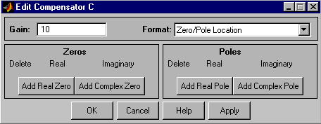
Note: As mentioned in text, you could do all the plotting below using sisotool. But using the statements are much(!) faster and probably more instructive while you are learning the root locus concept the first time.

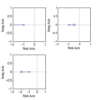
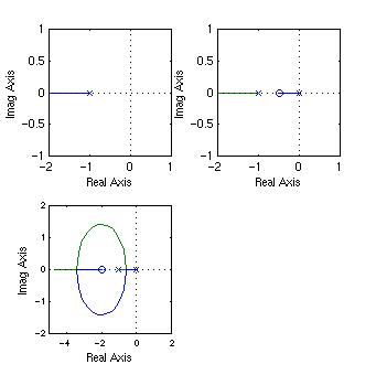
>> %Root locus plots of sample control systems
>> %First, a first order open-loop process and P and PD controllers
>> Gp=tf(1,[1 1]);    % open loop pole at -1, and Gc = Kc
>> subplot(221), rlocus(Gp)
>> taud=2;    % open loop zero at -1/2
>> Gc=tf([taud 1],1);
>> subplot(222), rlocus(Gc*Gp)
>> taud=1/2;    % open loop zero at -2
>> Gc=tf([taud 1],1);
>> subplot(223), rlocus(Gc*Gp)

>> %Plots for PI controllers
>> figure(2)
>> subplot(221), rlocus(Gp) % repeat Gc=Kc
>> taui=2; % open loop zero at -1/2
>> Gc=tf([taui 1],[taui 0]);
>> subplot(222), rlocus(Gc*Gp)
>> taui=1/2; % open loop zero at -2
>> Gc=tf([taui 1],[taui 0]);
>> subplot(223), rlocus(Gc*Gp)

>> %An ideal PID controller
>> figure(3)
>> subplot(221), rlocus(Gp) % repeat Gc = Kc
>> op_pole=[0]; % open loop pole at 0
>> op_zero=[-0.3 -0.8]; % both zeros "less" than -1
>> Gc=zpk(op_zero,op_pole,1);
>> subplot(222), rlocus(Gc*Gp)
>> op_zero=[-1.5 -3]; % both zeros "larger" than -1
>> Gc=zpk(op_zero,op_pole,1);
>> subplot(223), rlocus(Gc*Gp)
>> op_zero=[-0.5 -1.8]; % one zero in each region
>> Gc=zpk(op_zero,op_pole,1);
>> subplot(224), rlocus(Gc*Gp)

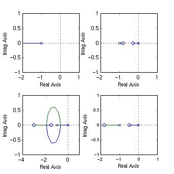
>> %Control systems with a second order overdamped open-loop process
>> %First, P and PD controllers
>> figure(1)
>> p=poly([-1 -2]); % open loop poles -1, -2
>> Gp=tf(1,p);
>> subplot(221), rlocus(Gp) % proportional control
>> taud=2; % open loop zero at -1/2
>> Gc=tf([taud 1],1);
>> subplot(222), rlocus(Gc*Gp)
>> taud=2/3; % open loop zero at -1.5
>> Gc=tf([taud 1],1);
>> subplot(223), rlocus(Gc*Gp)
>> taud=1/3; % open loop zero at -3
>> Gc=tf([taud 1],1);
>> subplot(224), rlocus(Gc*Gp)

>> %PI controllers
>> figure(2)
>> subplot(221), rlocus(Gp) % re-do proportional control
>> taui=2; % open loop zero at -1/2
>> Gc=tf([taui 1],[taui 0]);
>> subplot(222), rlocus(Gc*Gp)
>> taui=2/3; % open loop zero at -1.5
>> Gc=tf([taui 1],[taui 0]);
>> subplot(223), rlocus(Gc*Gp)
>> taui=1/3; % open loop zero at -3
>> Gc=tf([taui 1],[taui 0]);
>> subplot(224), rlocus(Gc*Gp)