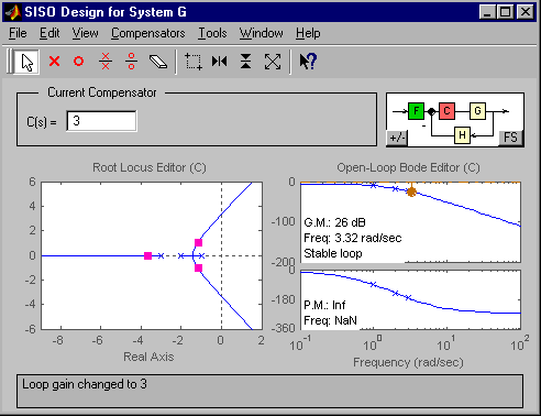
First a reminder following Session 6 about the availability of the nice SISO graphics design tool:
>> sisotool
The default view includes both the root locus and Bode plots. An illustration after importing a third order function is shown below. As you vary the position of the closed-loop poles (the red squares in the root locus plot), the Bode plot will be updated instantaneously (adjusting to the corresponding loop gain and reporting the new gain and phase margins).
We don't need to say more as the graphics tool is well designed and intuitive. Use the on-line Help if in case you have the need to.
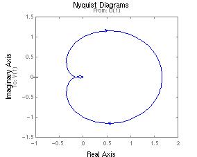
>> %Polar (Nyquist) plots
>> p=poly([-1; -2; -3]);
>> G=tf(10,p);
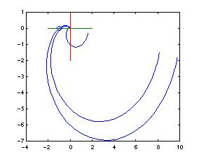
>> nyquist(G);
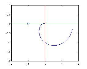
>> %We'll do our own plot, mapping only the positive
imaginary axis
>> [re,im,w]=nyquist(G);
>> plot(re(1,:),im(1,:))
>> w=logspace(-1,1);
>> [re,im]=nyquist(G,w);
>> plot(re(1,:),im(1,:))
>> hold
Current plot held
>> x=-1; y=0; %Add the (-1,0) point and
the axes
>> xh=[-2 2]; yh=[0 0];
>> xv=[0 0]; yv=[-2 1];
>> plot(x,y,'o',xh,yh,'-',xv,yv,'-')
>> %Calculation of gain and phase margins
>> %Option 1
Note: We are still doing calculations
based on G=tf(1,[1 0.4 1]). This is a simple second order system
that will not become unstable. Yes, the MATLAB
result is meaningless. We do it anyway just to underscore the point that
MATLAB won't even give you a warning if you are doing calculations that
are meaningless.
>> [Gm,Pm, Wcg,Wcp]=margin(mag,phase,w)
Gm =
652.8328 %<--meaningless results, and unit is absolute, not dB
Pm =
33.1675
Wcg =
25.4255
Wcp =
1.3573
>> %Option 2
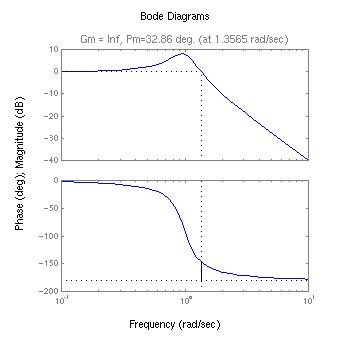
>> [Gm,Pm, Wcg,Wcp]=margin(G)
Gm =
Inf %<--This is a better telltale sign that the system is always stable
Pm =
32.8599
Wcg =
NaN
Wcp =
1.3565
>> %Option 3
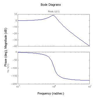
>> margin(G)
>> %To handle systems with dead time:
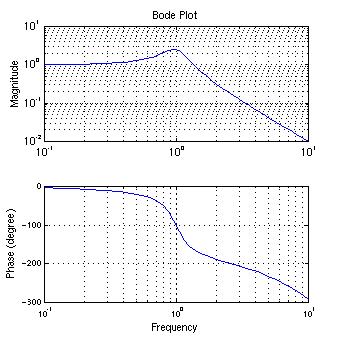
>> G=tf(1,[1 0.4 1]);
>> freq=logspace(-1,1);
>> [mag,phase]=bode(G,freq);
>> mag=mag(1,:);
>> phase=phase(1,:);
>> tdead=0.2;
>> phase = phase - ((180/pi)*tdead*freq); % phase
is in degrees
>>
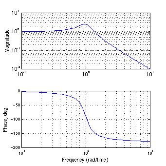
>> subplot(211), loglog(freq,mag)
>> ylabel('Magnitude'),title('Bode
Plot')
>> grid
>> subplot(212), semilogx(freq,phase)
>> ylabel('Phase (degree)'),xlabel('Frequency')
>> grid
Gm =
2.0432 %<--The unit is absolute, not dB
Pm =
17.6017 %<--The phase margin is a bit small, but this system is stable
Wcg =
1.7112
Wcp =
1.3573
>> %Optional reading based on Web Supplement--
redundant calculations to see that
>> %
there is no magic behind those MATLAB functions
>>
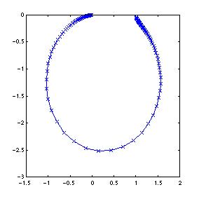
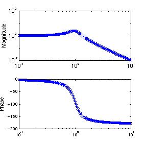
>> G=tf(1,[1 0.4 1]);
>> w=logspace(-1,1,200); %Deviation
from text. Use 200 points for smoother curve
>> gjw=freqresp(G,w); %
does the s=jw calculation for each w
>> [re,im]=nyquist(G,w);
>>
>> plot(re(1,:),im(1,:))
>> hold
Current plot held
>> R=real(gjw(1,:)); %
Real and imaginary parts of gjw are identical to the nyquist() calculation
>> I=imag(gjw(1,:));
>> plot(R,I,'x')
>> hold off
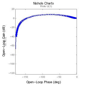
>> %Finally, we show that nichols() is just a
semilog plot of the magnitude versus phase angle
>> plot(phase(1,:),20*log10(mag(1,:)),'x')
>> title('Nichols Plot'),ylabel('Mag'),xlabel('Phase')
>> hold
Current plot held
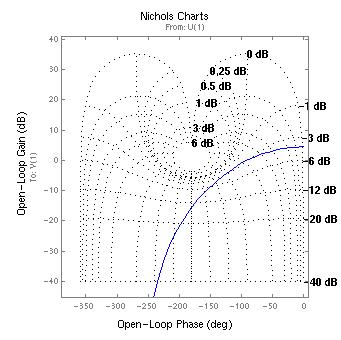
>> nichols(G)