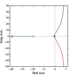
>> Gp=tf(0.8,[2 1])
Transfer function:
0.8
-------
2 s + 1
>> Gv=tf(0.9,[0.1 1])
Transfer function:
0.9
---------
0.1 s + 1
>> taui=0.05; %<--case 1
choice of
integral time constant for the PI controller function, Gi
>> Gi=tf([taui 1],[taui 0])
Transfer function:
0.05 s + 1
----------
0.05 s
>> rlocus(Gi*Gv*Gp) %You may want to zoom in the MATLAB window and get a better look near the origin
Transfer function:
0.5 s + 1
---------
0.5 s
>> rlocus(Gi*Gv*Gp)
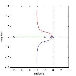
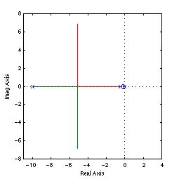
Transfer function:
5 s + 1
-------
5 s
>> rlocus(Gi*Gv*Gp)
>> %Part (e) - Find the ultimate gain
for
system without cascade control
>> taui=0.5;
>> Gi=tf([taui 1],[taui 0])
Transfer function:
0.5 s + 1
---------
0.5 s
>> Gvo=tf(0.5,[1 1]) %<--the valve function without cascade loop
Transfer function:
0.5
-----
s + 1
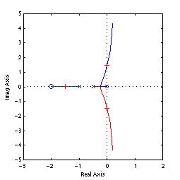
>> rlocus(Gi*Gvo*Gp)
%First we try root locus
>> zoom
>> rlocfind(Gi*Gvo*Gp) %find the ultimate gain
Select a point in the graphics window
selected_point =
0.0051 + 1.4617i
ans =
8.0799 %<--Very, very
sensitive to where you click even if you zoom in.
%
Values easy vary from 7 to 8.
(Analytical solution: should
be 7.5)
>> %Is there a better way? Definitely.
Let's
use a Bode plot.
>> margin(Gi*Gvo*Gp)
>> %MATLAB returns Gm=17.5 dB at 1.414
rad/s, Pm=31.5 deg at 0.5 rad/s
>> %And we know from Chapter 8 that this
so-called Gm is really the ultimate gain.
>> 10^(17.5/20)
ans =
7.4989 %<-- Yes, that's close enough to 7.5
>> %We can confirm that by using the
non-graphic (non-dB) result of the margin() function
>> [Gm,Pm, Wcg,Wcp]=margin(Gi*Gvo*Gp)
Gm =
7.5000
Pm =
31.4975
Wcg =
1.4142
Wcp =
0.5129
The reason why using cascade control stabilizes the system is best illustrated with frequency response analysis. So let's do the Bode plots first.
>> bode(Gi*Gv*Gp) %With cascade control valve function Gv. Blue line in
Bode
plot
>> hold
Current plot held
>> bode(Gi*Gvo*Gp) %Without cascade loop. Green line in Bode plot
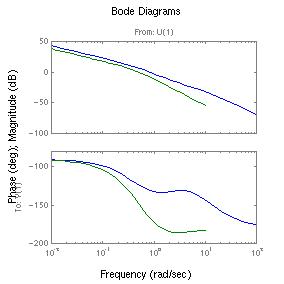
Note: sketch the low and high frequencies asymptotes on a piece of paper first before you read the following comments.
Without cascade control, the corner frequencies of the first order lags (time constants 2 and 1 s) are at 0.5 and 1 [rad/sec]. Together with the integrating function which contributes -90°, we can have a total phase lag of -270°. The PI controller lead term contributes a +90° at high frequencies, but with a corner frequency of 2 (taui = 0.5 s), it comes in too late.
With cascade control, the valve time constant is reduced from 1 to
0.1 s, so the corner frequency is "moved" from 1 out to 10. Now the
phase lead from the PI controller (corner freq 2 rad/s) is able to
cancel the phase lag
of the process function (corner frequency at 0.5) long before the
cascaded valve phase lag kicks in at 10 rad/c. So the total phase lag
never goes below
-180°.
Relative Gain Array Calculation
>> %The steady state gain array
calculation
of the blending problem
>> m1=0.1;
>> m2=10;
>> dum=(m1+m2)^2;
>> k11=m2/dum; %The gains are
calcuated with Eq. (10-30)
>> k12=-m1/dum;
>> k21=1; k22=1;
>> k=[k11 k12; k21 k22]; %The steady
state gains array, K
>> format long
>> k
k =
0.09802960494069 -0.00098029604941
1.00000000000000 1.00000000000000
>> format short
>> %The relative gain array calculation of the blending problem
>> %The numerical values are
based on
Example 10.3
>> %and specific to the blending
example
>> x=m1/(m1+m2);
>> L=[1-x x; x 1-x] %<--Eq.
(E10-6)
L =
0.9901 0.0099 %<--the relative gain array for the blending example
0.0099 0.9901
>> lamda=1-x %<--Eq. (E10-5)
lamda =
0.9901
Note 1: From Eq. (10-37), we should also calculate the relative gain using the more general formula based on steady state gains.
>> 1/(1 - k12*k21/k11/k22) %<--Eq. (10-37)
ans =
0.9901 %Yes,
It
is lamda
Note 2: The footnote mentioned (without proof) that if we know K, we can caluclate the relative gain array using the so-called Hadamard product.
k =
0.0980 -0.0010 %just repeating the result from above
1.0000 1.0000
>> k.*inv(k)' %<--element-by-element product of K with the transpose of its inverse
ans =
0.9901 0.0099 %<--Yes, same relative gain array that we obtained
earlier
0.0099 0.9901
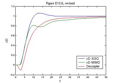
We now try to make Fig. E10.6. The three Simulink files to
generate the three curves are hiding in these links:
- e10_6siso.md,(does the xD-V
loop calculation),
- e10_6mimo.mdl (MIMO
calculation, set point change in xD), and
- e10_6decoup.mdl (adding
decouplers without changing controller settings)
Notes:
1. The PI controller settings that are "hard-wired" into the Simulink
files came from using the ITAE tuning relations (yes, from running
recipe.m).
2. The MIMO Simulink files have a step input to xB, but the numerical
value is set to zero; it is there just so you can experiment with
different changes. So now we are just looking into a set point change
in xD; its effect is a disturbance to xB.
3. We export the results to the Command Window workspace so we can plot
them. FYI, there are fancier ways to handle these calculations in
Simulink, but we decide to stay with the simple (and easy!) stuff.
 |
|
>> %After running the three Simulink
files, the SISO loop results are exported
>> %as
(t1,xd1), MIMO as (t2,xd2), and decoupler as (t,xd).
>> %The
final steps to make the plot are:
>> plot(t1,xd1, t2,xd2, t,xd);
>>
>> legend('xD SISO','xD MIMO','Decoupler')
>> xlabel('t'), ylabel('xD')
>> title('Figure E10.6, revised')