Chapter 2 MATLAB Results

The collection of MATLAB statements and screen display for:

Example 2.3

>> %Example 2.3
>> roots([1 1 -4 -4])

ans =

   -2.0000
    2.0000
   -1.0000

Example 2.4
>> %Example 2.4
>> [a,b,k]=residue([6 0 -12],[1 1 -4 -4])

a =

    1.0000    %Results returned by MATLAB provide no explanations
    3.0000    %That's why we say be careful when you interpret the results in the text
    2.0000
 

b =

    2.0000
   -2.0000
   -1.0000
 

k =

     []

Example 2.5
>> %Example 2.5
>> [a,b,k]=residue([6 0],[1 1 -4 -4])

a =

    1.0000
   -3.0000
    2.0000
 

b =

    2.0000
   -2.0000
   -1.0000
 

k =

     []

Example 2.6
>> %Example 2.6
>> p=poly([-1 -2 -3]);
>> [a,b,k]=residue(6,p)

a =

    3.0000
   -6.0000
    3.0000
 

b =

   -3.0000
   -2.0000
   -1.0000
 

k =

     []

Example 2.7
>> %Example 2.7
>> [a,b,k]=residue([1 5],[1 4 13])

a =

   0.5000 - 0.5000i
   0.5000 + 0.5000i
 

b =

  -2.0000 + 3.0000i
  -2.0000 - 3.0000i
 

k =

     []

Example 2.9
>> %Example 2.9
>> p=poly([-1 -1 -1 -2]);
>> [a,b,k]=residue(2,p)

a =

   -2.0000
    2.0000
   -2.0000
    2.0000
 

b =

   -2.0000
   -1.0000
   -1.0000
   -1.0000
 

k =

     []

Section 2.8

%Section 2.8.1 - See Review Problem 14 below

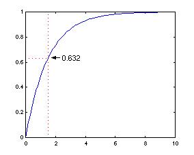
%Section 2.8.2 - We'll do an illustration on the typical unit step response of a first order function
>> t=0:0.1:10;
>> G=tf(1,[1.5 1]);   %We choose a function with steady state gain = 1 and time constant = 1.5
>> y=step(G,t);
>> plot(t,y)
>> hold
Current plot held
%We'll add red dotted lines to remind ourselves that when t = time constant, the step response is at 63.2%
%In the following plot, the time constant is 1.5 as stated above
%
>> plot([1.5 1.5],[0 1],'r:')  %the vertical line at 1.5
>> 1-exp(-1)

ans =

    0.6321

>> plot([0 1.5],[ans ans],'r:') %the horizontal line at 0.6321

Chapter 2 Review Problems

Review Problem 6
>> %Check the analytical results of No. 6
>> [a,b,k]=residue(6,[1 1 -4 -4])

a =

    0.5000
    1.5000
   -2.0000
 

b =

    2.0000
   -2.0000
   -1.0000
 

k =

     []

Review Problem 9
>> %Solve the matrix equation in No. 9,
>> %which is an alternate (and slower!) way of doing Example 2.9
>> a=[1 0 0 1; 4 1 0 3; 5 3 1 3; 2 2 2 1];
>> b=[0; 0; 0; 2];
>> a\b

ans =

    2.0000
   -2.0000
    2.0000
   -2.0000

Review Problem 11
>> %Partial fraction in No. 11
>> p=conv([1 0 0],[1 4 -5]);
>> roots(p)    %Make a habit of checking the roots

ans =

     0
     0
    -5
     1

>> [a,b,k]=residue([1 1],p)

a =

    0.0267
    0.3333
   -0.3600
   -0.2000
 

b =

    -5
     1
     0
     0
 

k =

     []
Review Problem 13 (Section 2.8.1)
>> %Simulations in No. 13
>> tau1=200;
>> G1=tf(1,[tau1 1]);
>> pulselength=10;
>> delt=5;
>> t=0:delt:1000;
>> u=zeros(size(t));
>> u(1:pulselength/delt+1)=5;
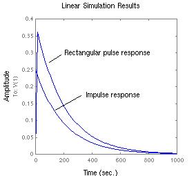
>> lsim(G1,u,t);    %The response of the rectangular pulse
>> hold
Current plot held
>> y=50*impulse(G1,t);   %Add on the impulse response
>> plot(t,y)
Note: if you have trouble, reverse the plotting order of the two curves. With an impulse
input, the response rises to a nonzero value instantaneously and then it decays exponentially.
>> %Now the response of two vessels
>> tau2=150;
>> G2=tf(1,[tau2 1]);
>> G=G1*G2;
>> lsim(G,u,t)
>> y=50*impulse(G,t);
>> hold
Current plot held
>> plot(t,y)
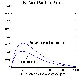
Note: The plot below takes a bit extra work to make it look nicer.