Note: You can use Simulink to do all these simulations too. In
that case, you can use the results here to
check that your block diagram is set up properly.
>> %Example 5.6
>> kc=1; %The two tuning parameters to be varied
>> taui=10;
>>
>> Gc=tf(kc*[taui 1],[taui 0]); %
The PI controller function
>> Gp=tf(0.8,[5 1]); %
The process function
>> Gcl=feedback(Gc*Gp,1) %
Unity feedback loop function GcGp/(1 + GcGp)
Transfer function:
8 s + 0.8
-------------------
50 s^2 + 18 s + 0.8
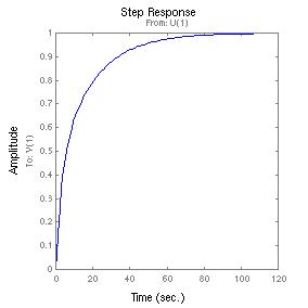
>> step(Gcl);
>> %Not too exciting, but this is the closed-loop
response to a unit step change in set point
>> %Review Problem 4 - decay ratio calculations
using Eqs. (5-17) and (5-18)
>> %Starting with a damping ratio
>> z=0.707;
>> DR=exp(-2*pi*z/sqrt(1-z*z))
%Eq.
(5-17) calculates the decay ratio
DR =
0.0019
>> OS=sqrt(DR)*100 %Percent overshoot
OS =
4.3255
>> dum=(log(DR))^2; %Now
use Eq. (5-18) to go backward and double check
>> z=sqrt(dum/(4*pi*pi+dum))
z =
0.7070
>> %What is the damping ratio when the decay ratio
is 1/4?
>> DR=0.25;
>> dum=(log(DR))^2;
>> z=sqrt(dum/(4*pi*pi+dum))
z =
0.2155
>> %And the percent overshoot when DR=0.25 is
(obviously!)
>> OS=sqrt(DR)*100
OS =
50
>> %Review Problem 7 - Repeat Example 5.6 closed-loop
simulation with a PI controller
>> %We first put the following statements from
Example 5.6 in an M-file named "pic.m"
Gc=tf(kc*[taui 1],[taui 0]);>> %Now we are ready to repeat the calculations with different values
Gp=tf(0.8,[5 1]);
Gcl=feedback(Gc*Gp,1)
step(Gcl);
Transfer function:
8 s + 0.8
-------------------
50 s^2 + 18 s + 0.8
>> hold
Current plot held
>> kc=5;
>> pic
Transfer function:
40 s + 4
-----------------
50 s^2 + 50 s + 4
>> kc=10;
>> pic
Transfer function:
80 s + 8
-----------------
50 s^2 + 90 s + 8
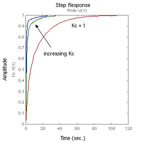
>> %We should get the following plot
>> %See that the system response is overdamped
faster with larger Kc
Transfer function:
8 s + 0.8
-------------------
50 s^2 + 18 s + 0.8
>> hold
Current plot held
>> taui=5; %Now use smaller integral time
constants
>> pic
Transfer function:
4 s + 0.8
------------------
25 s^2 + 9 s + 0.8
>> taui=3;
>> pic
Transfer function:
2.4 s + 0.8
--------------------
15 s^2 + 5.4 s + 0.8
>> taui=1;
>> pic
Transfer function:
0.8 s + 0.8
-------------------
5 s^2 + 1.8 s + 0.8
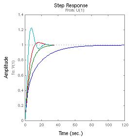
>> %We should get the following plot
>> %See that the system response becomes underdamped
when
>> %the integral time constant is small enough
ans =
-0.1800 + 0.3572i
-0.1800 - 0.3572i
>> damp(Gcl) %Use MATLAB to find the damping ratio of the closed-loop function
Eigenvalue Damping Freq. (rad/s)
-1.80e-01 + 3.57e-01i 4.50e-01
4.00e-01
-1.80e-01 - 3.57e-01i 4.50e-01
4.00e-01
>> z=0.45; %Let's check the
decay ratio and overshoot of the calculation
>> DR=exp(-2*pi*z/sqrt(1-z*z))
DR =
0.0422
>> os=sqrt(DR)*100 %Percent overshoot
os =
20.5346 %This value is
indeed what we see in the plot (the most underdamped curve)