Controller settings based on using
a first order with dead time function
Summary of results for (K, tau, td): (1.25, 4.00, 0.90)
Kc taui taud
------------ -----
---- ---- %Only selected lines of output retained
here...
Cohen-Coon PID 4.94 2.03 0.314
Ziegler-Nichols PID 4.27 1.8 0.45
ITAE(SP) PID 2.76 5.24
0.308
IMC PID
3.39 4.45 0.404
Ciancone (SP) PID 1.18 4.44 0.0737 %These selected lines are used in Examples 5.7A and B
Note on ciancone.m: This M-files is written to calculate the settings of a PI or PID controller based on a first order with dead time process reaction curve function [R. Ciancone and T. Marlin, "Tune controllers to meet plant objectives," Control 5, 50-57 (1992); also in Chapter 5 of Marlin]. This correlation is not in the text because the Ciancone relations are graphical and there is no point in printing that when we can't use it. You can see all the Ciancone tuning relation plots if you enter at the MATLAB prompt, simply:
>> ciancone
All the interpolation calculations are done within ciancone.m for you when you run recipe.m or ciancone.m with input arguments. Can enter "help ciancone" for more details.
You should find the Ciancone tuning relations to be extremely conservative, and the PID controller under most circumstances is really like a PI controller.
Note: You can use Simulink to do all these simulations too. In that case, you can use the results here to check that your block diagram is set up properly. There is a trade off. Simulink can handle the dead time term accurately (don't need the Pade approximation in the M-file below), but of course it runs a lot slower.
>> %Example 5.7C and Review Problem
>> %As suggested in Example 5.7C, we put the following
statements
>> %in an M-file, which we named "ex57.m"
alfa=0.1;>> %We can now do the time response simulations with the controller
Gc=tf(kc*[taui*taud (taui+taud) 1],[alfa*taui*taud taui 0]);
td=0.725;
Gm=tf([-td/2 1],[td/2 1]);
Km=2.6;
Gp=tf(0.8,[4 1]);
Ga=tf(0.6,[0.2 1]);
Gcl=feedback(Km*Gc*Ga*Gp,Gm);
step(Gcl)
>> kc=4.9; taui=2; taud=0.31; %Begin with
the Cohen-Coon tuning
>> ex57
>> hold
Current plot held
>> tspec(Gcl) %tspec is our own M-file which you can download from the
M-file list
Estimated dynamic response characteristics:
Peak time = 1.102
Percent overshoot = 73.54 Rough est. of decay ratio = 0.5408
Rise time = 0.4576
Settling time = 6.084
>> kc=4.3; taui=1.8; taud=0.45; %Ziegler-Nichols
tuning
>> ex57
>> tspec(Gcl)
Estimated dynamic response characteristics:
Peak time = 0.9743
Percent overshoot = 64.39 Rough est. of decay ratio = 0.4147
Rise time = 0.4213
Settling time = 4.279
>> kc=2.8; taui=5.2; taud=0.31; %ITAE
(Set point)
>> ex57
>> tspec(Gcl)
Estimated dynamic response characteristics:
Peak time = 1.84
Percent overshoot = 1.695 Rough est. of decay ratio = 0.0002873
Rise time = 1.505
Settling time = 7.08
>> % IMC with system time constant = 2/3*dead
time, the default setting inside recipe.m
>> kc=3.39; taui=4.45; taud=0.404;
>> ex57
>> tspec(Gcl)
Estimated dynamic response characteristics:
Peak time = 1.187
Percent overshoot = 11.72 Rough est.
of decay ratio = 0.01373
Rise time = 0.7761
Settling time = 3.242
>> kc=1.2; taui=4.4; taud=0.07; %Ciancone
(Set point)
>> ex57
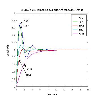
>> %This is the plot that you should see.
>> %Cohen-Coon is the most underdamped, and Ciancone
is the most conservative.