
>> %Example 7.4 - numerical root finding of
the ultimate frequency
>> %As suggested in the example, we put these
two statements in
>> %an M-file named 'f.m'
function y=f(x)>> fzero('f ',0.9)
y = 5*x + tan(2*x);
ans =
0.8953
>> fzero('f
',0.8)
Zero found in the interval: [0.77737, 0.8].
ans =
0.7854
>> pi/4
ans =
0.7854
>> %Example 7.2B - redo Example 7.2 with root
locus
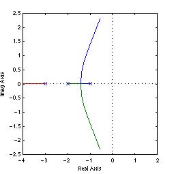
>> G=zpk([],[-1 -2 -3],1);
>> k=0:1:100; %The MATLAB
default won't cross the Im-axis.
>> rlocus(G,k) %We have to use our own gain vector in this example
selected_point =
0.0025 + 3.3099i %<--bit off the Im-axis
ans =
59.7885 %<--that's pretty
close to 60, what we derived in Example 7.3
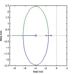
>> %Example 7.3B - back to analysis Example
7.3 with root locus
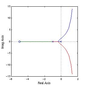
>> taui=0.2; %Open-loop zero at -5
>> G=tf([taui 1],conv([taui 0],[1
2 1]));
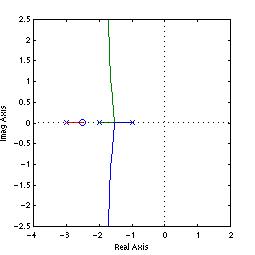
>> rlocus(G)
>> %Reminder: the root locus may look funny.
That's because we
>> %have two repeated open-loop poles at
-1.
| Note on the root locus plot |
| This root locus plot appears to be one continuous
line on the real axis, but it is not. Note the color change.
The result is due to the double pole at -1. We have one locus moving
to the open-loop zero at -5, and another toward the Im-axis to
eventually form the complex loci. |
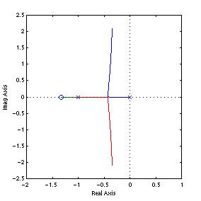
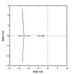
>> %Now pick an integral time larger than
0.5. See if indeed
>> %the system is always stable
>> taui=0.75;
>> G=tf([taui 1],conv([taui 0],[1
2 1]));
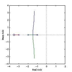
>> rlocus(G)
| Note on the use of rlocfind() |
| There are situations that you'll find
the region around the Im-axis very small and you need to zoom in to get
a better look. Activate zoom by the zoom command or by the
zoom button in the Figure Window. Once zoom is activated, we can left-mouse-click
to zoom in; right-mouse-click zooms out. Of course, we zoom in and toggle
the zoom off (say with the zoom button) before doing the rlocfind().
And with the new MATLAB, we can skip the use of rlocfind() entirely. Just click on a locus and drag the little black square that appears. (See also Post-It comment in MATLAB Session 6.) |
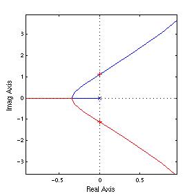
selected_point =
0.0038 + 1.1142i %<--the
selected point is a bit off,
% not exactly on the Im-axis
ans =
0.2490 %<--
that's close enough to 0.25 to say that
% the different
methods give the same results
>> zoom off %<--don't forget to turn zoom off
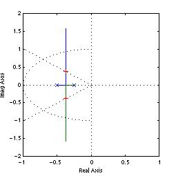
selected_point =
-0.3788 + 0.3770i
kc =
1.2621 %<--not the
same as 1.29 when I first did it in the text.
% You may want to zoom
in when you do it.
cpole =
-0.3750 + 0.3770i
-0.3750 - 0.3770i
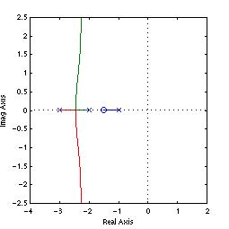
| Warning on the rlocus() interactive feature |
| If we click on a locus and drag the little black
square that appears, MATLAB reports the overshoot. The value is based on
a simple second order function with no zeros. So the value will
not be correct as in the case of Example 7.7 where the closed-loop
function has a zero due to the PD control. In Example 7.7, we should find the OS of the lower gain pair of roots not too different from a pure second order function -- the position of these poles is only slighlty off from a "vertical line" locus expected of a simple 2nd order system. Now the higher gain pair of roots lie far away from the "vertical 2nd order locus" and we expect a much larger error. Indeed, if we do a time response simulation, the system wtih the higher gain has over 10% OS. |
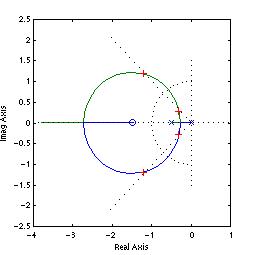
selected_point =
-0.3194 + 0.3155i
kc =
0.5342 %<--bit off
from text when I first did it;
% you may want to zoom
it when you do it
cpole =
-0.3168 + 0.3162i
-0.3168 - 0.3162i
>> [kc,cpole]=rlocfind(G) %clicking point with higher Kc
Select a point in the graphics window
selected_point =
-1.1528 + 1.1621i
kc =
7.1955 %<--bit off from text when I first did it
cpole =
-1.1494 + 1.1735i
-1.1494 - 1.1735i