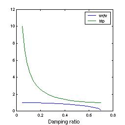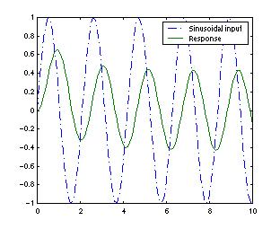
>> %You may wonder how to make Figure 8.1. Here's an illustration.
>> G=tf(2,[1.5 1]) %Just an arbitrary first order function
Transfer function:
2
---------
1.5 s + 1
>> t=0:0.1:10;
>> freq=3;
>> u=sin(freq*t);
%Make a sine function and do the simulation
>> y=lsim(G,u,t);
%as we did once in MATLAB Session 3
>> plot(t,u,'-.', t,y);
>> legend('Sinusoidal input','Response')
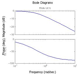
>> %Example 8.2 - First order function
>> kp=1; % Just some arbitrary values
>> tau=2;
>> G=tf(kp,[tau 1]);
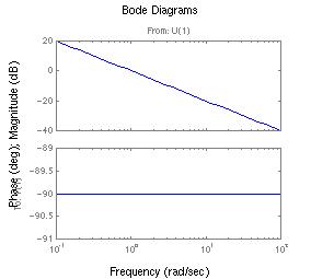
>> figure(1), bode
(G);
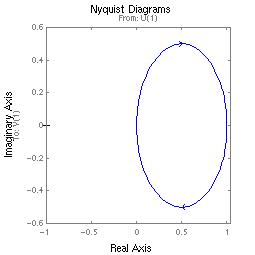
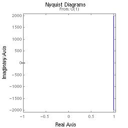
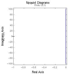
>> figure(2), nyquist
(G);
>> %MATLAB default Nyquist plot maps the entire
Im-axis; hence the circle
| Note on Bode plots |
| --With computer generated plots,
it is never easy to identify the slope of the magnitude asymptote
unless you use a print out. It is much easier to identify the phase
lag at low and high frequencies. --Also, keep in mind that if a function is in pole-zero form, any "gain" is not the steady-state gain. You need the time-constant form for that. |
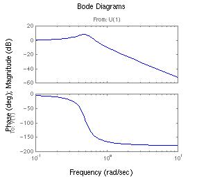
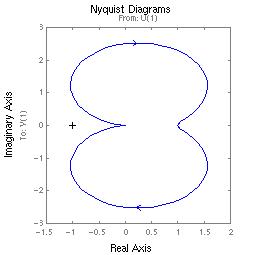
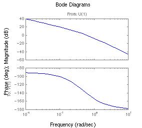
>> %Example 8.3 - Second order underdamped
function
>> k=1;
>> tau=2;
>> zeta=0.2;
>> G=tf(k,[tau*tau 2*zeta*tau 1]);
>> damp(G)
Eigenvalue Damping Freq. (rad/s)
-1.00e-01 + 4.90e-01i 2.00e-01
5.00e-01
-1.00e-01 - 4.90e-01i 2.00e-01
5.00e-01
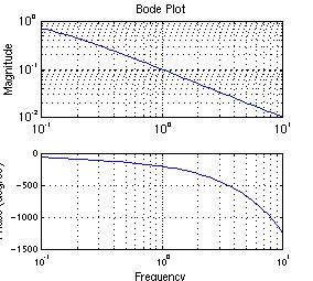
>> figure(1),
bode(G);
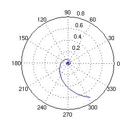
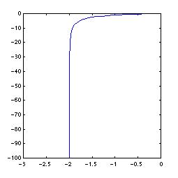
>> figure(2), nyquist
(G);
>> figure(1);
>> subplot(211),
loglog(freq,mag)
>> ylabel('Magnitude'),
title('Bode Plot'), grid
>> subplot(212),
semilogx(freq, phase)
>> ylabel('Phase (degree)'),
xlabel('Frequency'), grid
>> figure(2)
%Use the polar plot function for the Nyquist diagram here
>> phase=phase*pi/180;
>> polar(phase,mag)
>> %Example 8.9 - Bode plot of a complex function
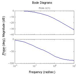
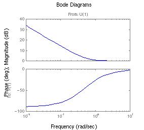
>> G=tf([5 1], conv
([10 1],[2 1]));
>> bode(G);
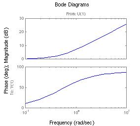
>> %Example 8.11 - Ideal PD versus a real
PD controller
>> kc=1;
>> taud=2;
>> G=tf(kc*[taud 1],1);
%The ideal PD controller
>> figure(1), bode
(G)
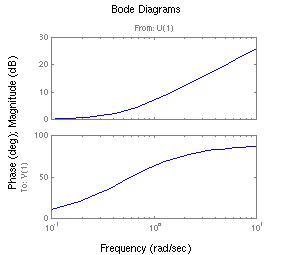
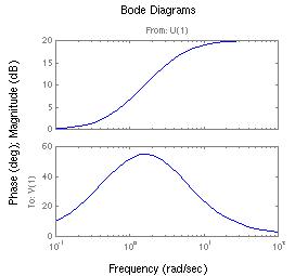
>> G=tf(kc*[taud 1],[0.1*taud 1]) %Now the real PD controller (not in the text example)
Transfer function:
2 s + 1
---------
0.2 s + 1
>> figure(2), bode(G)
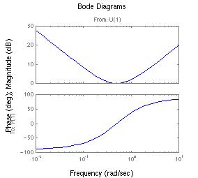
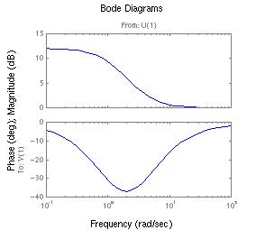
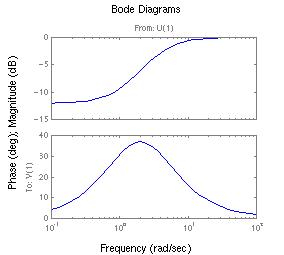
>> %Example 8.13 - Phase-lead versus phase-lag
compensator
>> kc=1;
>> zo=4;
>> po=1;
>> G=zpk(-zo,-po,kc);
%This is the phase-lag compensator
>> figure(1), bode
(G)
>> %Example 8.14 - Choice of phase-lead vs.
phase-lag compensator with a first order process in a system
>> Kp=1;
>> taup=1;
>> Gp=tf(Kp,[taup 1])
%First order function with some arbitrary values
Transfer function:
1
-----
s + 1
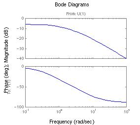
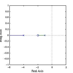
>> %part (a) Phase-lead compensator
>> zo=2;
>> po=4;
>> Gc=zpk(-zo,-po,1)
Zero/pole/gain:
(s+2)
-----
(s+4)
>> figure(1),
bode(Gc*Gp) %Phase-lead with the first order
process function in a system
>> figure(2), rlocus
(Gc*Gp)
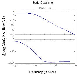
>> %part (b) Phase-lag compensator
>> zo=4;
>> po=2;
>> Gc=zpk(-zo,-po,1)
Zero/pole/gain:
(s+4)
-----
(s+2)
>> figure(1),
bode(Gc*Gp) %Phase-lag with the first order
process function in a system
>> figure(2), rlocus
(Gc*Gp)
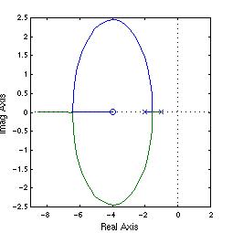
>> %Example 6.2C - repeat Example 6.2 with
frequency response analysis
>> p=poly([-1 -2 -3]);
>> G=tf(1,p);
>> margin(G);
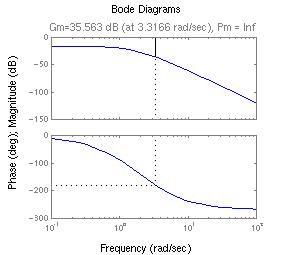
>> %Ultimate gain based on the "Gm" of this
plot
>> 10^(35.56/20)
ans =
59.9791 %<-- that's essentially 60, what we got in Example 6.2
>> kc=60/1.7 %so we round the number up to 60
kc =
35.2941 %That's the proportional gain if we want a GM of 1.7
>> G=tf(kc,p);
%calculations to double check if that it is correct
>> margin(G)
>> %We'll skip the plot here, but it's just like
the one above.
>> %The values returned in the MATLAB figure are
Gm=4.609 dB and Pm=18.8 deg
>> 10^(4.609/20)
ans =
1.7000
>> %The next item is to find better controller
settings using the Ziegler-Nichols relations
>> %And using our own M-file
>> recipe(60,3.32)
(NZ) P only:
Kc = 30
(NZ) PI controller:
Kc = 27.3 taui= 1.58
>> G=tf(30,p);
%First check the case if we use a P controller
>> margin(G)
>> %MATLAB returns Gm=6 dB and Pm=25.4 deg (Note:
6 dB is exactly Gm=2)
>> kc=27.3; taui=1.58; %Now the PI controller
>> p2=conv(p,[taui 0]);
>> G2=tf(kc*[taui 1],p2);
>> margin(G2)
>> %MATLAB returns Gm=3.356 dB, Pm=12.3 deg
>> 10^(3.356/20)
ans =
1.4716
>> %Finally, try to detune the PI controller,
keeping the same integral time constant
>> %First step, find the new ultimate gain with
this PI controller
>> kc=1; taui=1.58;
>> p2=conv(p,[taui 0]);
>> G2=tf(kc*[taui 1],p2);
>> margin(G2);
>> %MATLAB returns Gm=32.08 dB at 2.77 rad/s;
Pm=88.4 deg at 0.11 rad/s
>> 10^(32.08/20)
ans =
40.1791 %<--this is the new ultimate gain
>> kc=40.18/2; %Choosing a gain margin
of 2
>> G2=tf(kc*[taui 1],p2);
%just a double check
>> margin(G2)
>> %MATLAB returns Gm=6 dB, Pm=23.2 deg
tmp =
0.1000 0.1655 -10.4822
...deleted...
1.0826 0.0935 -95.5432
1.3738 0.0735 -113.0399
1.7433 0.0540 -131.3995
%<-- the numbers that we use below
2.2122 0.0371 -149.9648
... rest deleted
>> %Calculations based on the values at 1.74
rad/s
>> kc=1/0.054
kc =
18.5185
>> G=tf(kc,p); %Now repeat the
system calculation
>> margin(G)
>> %MATLAB returns Gm=10.2 dB and Pm=48.6 deg
>> 10^(10.2/20)
ans =
3.2359
>> %Calculations based on the values at 2.21
rad/s
>> kc=1/0.0371
kc =
26.9542
>> G=tf(kc,p);
>> margin(G)
>> %MATLAB returns Gm=6.95 dB, Pm=30.1 deg
>> 10^(6.95/20)
ans =
2.2259
>> %Example 7.4A - redo Example 7.4 with frequency
response technique
>> G=tf(0.8,[5 1]);
>> tdead=2;
>> [Mag,Phase,freq]=bode(G);
>> Mag=Mag(1,:);
>> Phase=Phase(1,:) - ((180/pi)*tdead*freq');
>> [Gm,Pm,Wcg,Wcp]=margin(Mag,Phase,freq)
Gm =
5.7232
note ....other MATLAB printouts deleted
>> %Now to use a gain margin of 1.7
>> kc=Gm/1.7
kc =
3.3666
>> G=tf(kc*0.8,[5 1]);
%And repeat the margin calculations to double check
>> [Mag,Phase,freq]=bode(G);
>> Mag=Mag(1,:);
>> Phase=Phase(1,:) - ((180/pi)*tdead*freq');
>> [Gm,Pm,Wcg,Wcp]=margin(Mag,Phase,freq)
Gm =
1.7000 %<--indeed
note ....other MATLAB printouts deleted
Note: If you hate to retype all these statements when there is dead time in the problem, download from the M-file list ezbo.m. The necessary statements are in there and you can modify it for your own use. We'll skip that in Example 5.7D below just so we see every single MATLAB statements.
>> %Example 5.7D - the real calculations begin
>> %Part (b). Find the gain margin of the approximate
problem when dead time is reduced to 0.725
>> %The calculation here is meant to compare with
Part (a), so we'll use the reduced order model
>> k=5;
>> tdead=1.45/2;
>> taup=4; %The large time constant; dominant
pole is at 1/4
>> G=tf(k,[taup 1])
Transfer function:
5
-------
4 s + 1
>> %MATLAB default is no good, need to force
it to use higher frequencies for margin interpolation later
>> freq=logspace(-1,1)'; %And don't
forgot the transpose '
>> [Mag,Phase]=bode(G,freq);
>> Mag=Mag(1,:);
>> Phase=Phase(1,:) - ((180/pi)*tdead*freq');
>> [Gm,Pm,Wcg,Wcp]=margin(Mag,Phase,freq)
Gm =
1.8611
note ....other MATLAB printouts deleted
>> %Part (c)
>> %We now redo the ultimate gain calculation
properly with the given transfer functions
>> k=0.8*0.6*2.6
k =
1.2480
>> G=tf(k, conv([0.2 1],[4 1]))
Transfer function:
1.248
-------------------
0.8 s^2 + 4.2 s + 1
>> tdead=0.725;
>> freq=logspace(-1,1)';
>> [Mag,Phase]=bode(G,freq);
>> Mag=Mag(1,:);
>> Phase=Phase(1,:) - ((180/pi)*tdead*freq');
>> [Gm,Pm,Wcg,Wcp]=margin(Mag,Phase,freq)
Gm =
6.4153
Pm =
133.4649
Wcg =
1.8592
Wcp =
0.1861
>> Gm/1.7 %To find the proportional gain for a gain margin of 1.7
ans =
3.7737
>> %Part (d). Use the Ziegler-Nichols ultimate-gain
tuning relations
>> recipe(6.42,1.86)
___ The Ziegler-Nichols Ultimate-Gain Method __
(NZ) PID controller for 1/4 decay:
Kc = 3.77 taui= 1.69 taud= 0.422
(NZ) PID controller for slight overshoot:
Kc = 2.14 taui= 1.69 taud= 1.12
(NZ) PID controller for no overshoot:
Kc = 1.28 taui= 1.69 taud= 1.12
>> %We now repeat the time response simulations
in Example 5.7C
>> %We also will re-use the M-file
ex57.m created back then (See Examples in Chapter
6)
>> %We also use, once again, our own M-file
tspec.m
>> kc=3.77; taui=1.69; taud=0.42;
%Z-N 1/4 decay ratio setting
>> ex57
>> tspec(Gcl)
Estimated dynamic response characteristics:
Peak time = 1.154
Percent overshoot = 51.32 Rough est. of decay ratio = 0.2634
>> kc=2.14; taui=1.69; taud=1.12;
%Z-N slight overshoot setting
>> hold
Current plot held
>> ex57
>> tspec(Gcl)
Estimated dynamic response characteristics:
Peak time = 0.8666
Percent overshoot = 27.22 Rough est. of decay ratio = 0.07408
>>
>> kc=1.28; taui=1.69; taud=1.12;
%Z-N no overshoot setting
>> ex57
>> tspec(Gcl)
Estimated dynamic response characteristics:
Peak time = 5.128
Percent overshoot = 8.144 Rough est.
of decay ratio = 0.006632
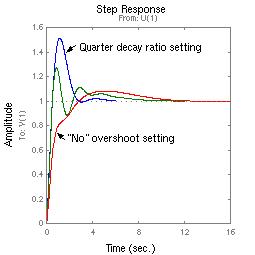
Note: You may wonder why the "no" overshoot setting curve looks
so weird. The hint is in the homework problems back in Chapter 2. The reason
is due to a complex pole which has a larger negative real part than the dominant
pole(s). So this complex pole decays away quickly, but it "exists" long enough
to give us the hump near the beginning.
>> %Final remarks with respect to an example
of a PID controller calculation
>> taui=3;
>> taud=0.5;
>> gc=tf([taui*taud (taui+taud) 1],[taui
0]); %ideal PID without the Kc
>> tdead=0.725;
>> k=0.8*0.6*2.6;
>> G=tf(k, conv
([0.2 1],[4 1]));
>> [Mag,Phase]=bode(gc*G,freq);
%<--note the change here
>> Mag=Mag(1,:);
>> Phase=Phase(1,:) - ((180/pi)*tdead*freq');
>> [Gm,Pm,Wcg,Wcp]=margin(Mag,Phase,freq)
Gm =
5.8697
note ....other MATLAB printouts deleted
>> kc=Gm/1.7 %<--what to use for a gain margin of 1.7
kc =
3.4528
>> ex57 %<--using taui=3, taud=0.5 defined above

>> tspec(Gcl)
Estimated dynamic response characteristics:
Peak time = 0.9796
Percent overshoot = 22.78 Rough est. of decay ratio = 0.05191
Rise time = 0.5714
Settling time = 4.517
Note: This is sufficiently long-winded! I bet you can proceed and try other ideas on your own from here.