Co =
0 0
1
0 1 -6
1 -6 25
>> Co=[B A*B A^2*B] %Compute with the definition itself
Co =
0 0
1
0 1 -6
1 -6 25
>> C=[1 0 0];
>> Ob=obsv(A,C)
%Find the observability matrix
Ob =
1 0
0
0 1
0
0 0
1
>> Ob=[C; C*A; C*A^2] %Compute with the definition itself
Ob =
1 0
0
0 1
0
0 0
1
>> %Example 9.2 - State feedback gain calculation
>> A=[0 1 0; 0 0 1; -6 -11 -6];
>> p1=poly(A)
p1 =
1.0000 6.0000 11.0000 6.0000
>> P=[-3+3j -3-3j -6];
>> p2=poly(P) %the
"alpha" coefficients
p2 =
1 12 54 108
>> p2-p1 %Ki as in Eq. (9-21)
ans =
0 6 43 102
>> %Now re-do using Ackermann's formula
>> B=[0; 0; 1];
>> acker(A,B,P)
ans =
102 43 6
>> %Redo Ackermann's formula using its definitions
>> M=[B A*B A^2*B]; %controllability
matrix
>> ac=polyvalm(p2,A);
%Eq.(9-23)
>> [0 0 1]*inv(M)*ac
%Eq.(9-22)
ans =
102 43 6
>> %Example 4.7B
>> % -- state feedback gain calculation
of the two CSTR-in-series
>> A=[-5 0; 2 -4];
>> B=[4; 0];
>> C=[0 1];
>> D=0;
>> rank(ctrb
(A,B)) %should find rank = 2 for both the
%controllability
observability matrices
ans =
2
>> rank(obsv (A,C))
ans =
2
>> [q,p]=ss2tf(A,B,C,D);
%converts state space to transfer function
>> Gp=tf(q,p);
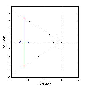
>> rlocus(Gp)
>> sgrid(0.8,1)
>> [kc,P]=rlocfind(Gp)
Select a point in the graphics window
kc =
1.4514 %That's
almost 1.46 used in text
P =
-4.5000 + 3.3706i %These are
the closed-loop poles that
-4.5000 - 3.3706i %
we'll use in the system design
>> K=acker(A,B,P)
K =
0 1.4514
>> %Example 4.7C, adding integral action to the control system
>> kc=1; taui=1/3;
>> Gc=tf(kc*[taui 1],[taui 0]);
>>
>> %Again, we first use root-locus to find us
the closed-loop poles
>> rlocus(Gc*Gp);
>> sgrid(0.8,1)
>> [kc,P]=rlocfind(Gc*Gp)
Select a point in the graphics window
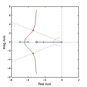
kc =
1.6761 %That's
almost 1.66 used in text
P =
-3.4214 + 2.6347i %These are
the closed-loop poles that
-3.4214 - 2.6347i %we'll use
in the system design
-2.1572
>> Ah=[A zeros(2,1); -C 0];
%Eq. (9-29)
>> Bh=[B; 0];
>> Kh=acker(Ah,Bh,P)
Kh =
0 1.6761
-5.0284
>> %Try the time-domain simulation to see
that there is no offset
>> Asys=Ah-Bh*Kh;
>> eig(Asys)
%Check the eigenvalues
ans =
-3.4214 + 2.6347i %Yes,
they are the same as the poles
-3.4214 - 2.6347i
-2.1572
>> Bsys=[0; 0; 1]; %Follows (9-28)
>> Csys=[C 0];
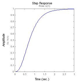
>> step(Asys, Bsys,Csys,0)
>> %Indeed the plot shows that the system has
no offset
>> %Example 7.5B - Do Example 7.5A (root locus
design) with state feedback
>> %First, make the state space object from the
transfer function
>> G=tf(1,conv
([2 1],[4 1]));
>> S=ss(G)
a =
x1 x2
x1
-0.75 -0.25
x2
0.5 0
b =
u1
x1
0.5
x2
0
c =
x1 x2
y1
0 0.5
%<--that's S.c, output matrix in reverse
indexing and
% not normalized as [0 1]
d =
u1
y1
0
Continuous-time model.
>> scale=S.c(2); %<--rescale
B and C as explained in MATLAB Session 4
>> S.c=S.c/scale;
>> S.b=S.b*scale
a =
x1 x2
x1
-0.75 -0.25
x2
0.5 0
b =
u1
x1
0.25
x2
0
c =
x1 x2
y1
0 1
%<-- S.c is now [0 1] and we are ready to
do find the feedback gains
d =
u1
y1
0
Continuous-time model.
>> P=[-0.375+0.382j -0.375-0.382j]; %Define
the closed-loop poles
>> K=acker(S.a,S.b,P)
K =
0 1.2924
%<-- We had obtained 1.29 with root locus in Example
7.5A
Example 7.5B. Time response simulation (as requested in Review Problems)
>> %To do the system response simulation,
we need the system matrices
>> %That's Eq. (9-25), except MATLAB reverses
the indexes
>> A = S.a - S.b*K
A =
-0.7500 -0.5731
0.5000
0
>> B = S.b*K(2) %MATLAB reversed the indexing
B =
0.3231
0
>> C = S.c
C =
0 1
>> D=0;
>> % Slight deviation in plotting steps so
we can overlay two curves nicely
>> [y,t]=step(A,B,C,D);
>>
>> Gcl=feedback(1.29*G,1);
%Kc=1.29 was the proportional gain obtained
>>
%in Example 7.5A
>> [y1,t1]=step(Gcl);
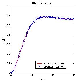
>> plot(t,y,'r', t1,y1,'x') %Here, both design
techniques are the same!
Ke =
21
106
-144
>> %Now check the eigenvalues
>> K=[102 43 6]; %Feeback gains calculated from
Example 9.2
>> A11=A-B*K; %Submatrices in Eq. (9-42)
>> A12=B*K;
>> A21=zeros(3,3);
>> A22=A-Ke*C;
>> BIGA=[A11 A12; A21 A22];
>> eig(BIGA)
ans =
-3.0000 + 3.0000i
-3.0000 - 3.0000i
-6.0000
-9.0000 + 0.0000i
-9.0000 - 0.0000i
-9.0000
Ker =
12
-2
Review Problem
>> %Adding integral action to Example 7.5B to eliminate the offset
>> G=tf(1,conv
([2 1],[4 1])); %Repeat
making the plant state space object
>> S=ss(G);
>> scale=S.c(2); %<--rescale B
and C
>> S.c=S.c/scale;
>> S.b=S.b*scale;
>> %We now make the integral control system
matrices as defined in Eq. (9-29)
>> Ah=[S.a zeros(2,1); -S.c 0]
%A-head in (9-29)
Ah =
-0.7500 -0.2500
0
0.5000
0 0
0 -0.5000
0
>> Bh=[S.b; 0] %B-head in (9-29)
Bh =
0.2500
0
0
>> %Define the closed-loop poles.
>> %We now add a faster (less dominant) pole at
-1 to the
>> %two desired complex poles in Example 7.5B
>> P=[-0.375+0.382j -0.375-0.382j -1];
>> kh=acker(Ah,Bh,P) %K-head in (9-29)
kh =
4.0000 7.2924 -2.2924
>>
>> %The last value kh(2) is -Kn+1 in text
introduced by the "integrator"
>>
>>
>> %Finally! Do the time response simulation to confirm that
>> %we have no steady state error
>> Asys=Ah-Bh*kh %Make the entire system matrix as in (9-29)
Asys =
-1.7500 -2.0731 0.5731
0.5000
0 0
0 -1.0000
0
>> eig(Asys) %Check the eigenvalues of Asys with both eig() and damp()
ans =
-1.0000
-0.3750 + 0.3820i %<--indeed
same as P that we defined above
-0.3750 - 0.3820i
>> damp(Asys)
Eigenvalue Damping Freq. (rad/s)
-3.75e-01 + 3.82e-01i 7.01e-01
5.35e-01
-3.75e-01 - 3.82e-01i 7.01e-01
5.35e-01
-1.00e+00
1.00e+00 1.00e+00
>> Bsys=[0; 0; 1] %Follows (9-28). The system B is NOT B-head.
Bsys =
0
0
1
>> Csys=[S.c 0] %Need be consistent with S.a and S.b
Csys =
0 1 0
>> step(Asys, Bsys,Csys,0)
>> %Yes, the steady state error is eliminated.
