If you do not need an introduction, this is the list of Simulink mdl files that we can provide as examples. Otherwise, jump to the introduction farther down the page.

Save these links as a file. You can open them from within a Simulink Window or by simply entering their name (without the ".mdl" extension) inside the Command Window.
• Simple loop example - A simple exercise
• PID - A simple SISO system using the ideal PID controller.
• PID2 - Another simple SISO system, but we build our own real PID controller with derivative action on the controlled variable. Added dead time in the feedback path too.
• Cascade - A simple system with the primary and secondary loops.
• Feedforward - A very simple loop with nothing but a feedforward controller. Should find that such a system is not too useful and meaningful.
• Feedforward-feedback - What we want is feedback trim to a feedforward controller. This is a simple set up for that.
• Simple loop with large dead time - Example used in the notes on Nyquist Stability Criterion listed on the Supplementary Notes page. It is a unity feedback loop that has an extremely large dead time.

>> simulink

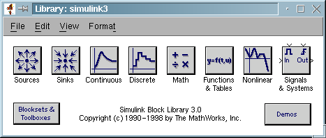
The Simulink Block Library window will pop up as shown below. The handy tools (models) are hiding in each of the icons. Double-click an icon will open up additional windows for each category of models.

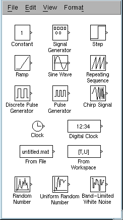
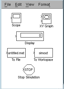
The first important question is: where can we find the models to build a block diagram that we usually use? We'll go through some of the more important icons in the main Block Library window. First are the Sources and Sinks.

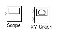
From the Sources (in the left panel) the most useful ones are the Constant, Step input, and the Clock for the time variable. In the Sinks (the right panel), we can use the "Scope" or the the "XY Graph" for plotting and "To Workspace" which can export a variable as an array into the workspace for analysis or plotting. The other features? Ignore them for now. Don't let them distract you.

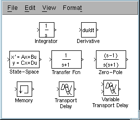
Just to the right of Sources and Sinks are the Continuous and Math icons. Double-click on them to open up their libraries.

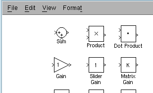
In the Continuous panel (on the left) are the very important transfer functions in either the polynomial or pole-zero forms. A model can also be built in state space representation. Many control engineers prefer to built differential equation models based on the 1/s integrator. We'll use the transfer functions instead; they are less flexible but they are cleaner and follow closer to the analyses in the text. Also availabe is transport Delay, which is what we use for dead time or time delay. In the Math panel (only top part shown on the right), we find the very important summing point, sum. Also handy are the Gain and Slider Gain for changing values between simulation runs.

 
We will not show them, but inside the Nonlinear icon of the Block Library, we can find Saturation and Dead Zone models. They can be handy to apply to the controller and actuating elements to simulate more real-life behavior.

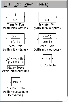
And you may ask: is there a PID controller? Yes. Double-click the Blocksets & Toolboxes icon in the main Block Library, then find the icon Simulink Extras, and finally Additional Linear. Near the bottom of this panel is the ideal PID Controller, and the (real) PID controller with approximate derivative.

Now that we know where things are hiding. How do we make use of them? Go under the File pull-down menu of any of the Simulink windows and open a new model. A blank "untitled" window will appear.

To build a block diagram, you go to the proper block library winow, click on the model, and drag-and drop the icon into your blank window. After that, don't forget to save your work. To connect the blocks, you click on the little arrow-like connectors of a block and move the mouse to another block's connector. It is not as smooth as a CAD program, but you'll get use to it after a couple of tries. In time, you can build a text-book closed-loop system as shown below.

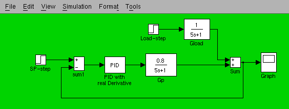
Refer to the text MATLAB Session 5 for additional comments about using Simulink. It is by and large a point-and-click venture; not much of a learning curve to it. Finally, make use of the Simulink section of the MATLAB On-line Help. There is a good reason why we provide only brief comments or why we should not have to waste money buying one of those MATLAB tutorial books. The MATLAB Help Browser is incredibly nice!

Finally, even with the Help Browser, here's a few tidbits that can help you. They are related to the models used in the simple closed-loop system shown above.
 

	To set the properties of the step input function, double-click on the icon. The default is a unit step that begins at t = 1 unit. That is the first data entry "Step time." Change the "Step time" to zero so the unit step starts at t = 0.
	To set the properties of the summing point, double-click on the icon. The default is "|++" and the instruction on how to change the sign and location is in the upper panel of the sum property dialog box. For the negative feedback loop summing point, we change the setting to "|+-" You can also change the shape of the summing point.
	To plot a simulation, the Scope is the easiest to use. Just feed it the data stream as shown in the block diagram above, in which we have changed its label to become "Graph." When you first run the simulation, double-click on the icon to open up its graphing window. Otherwise, nothing seems to happen. The graphing window has a nice tool set to modify the plot. You can also port more than one data stream into the Scope icon. As its name says, the XY Graph requires both x and y data. It is also not autoscale. Double-click on the icon to set its properties such as xmin, xmax, ymin, ymax, etc.

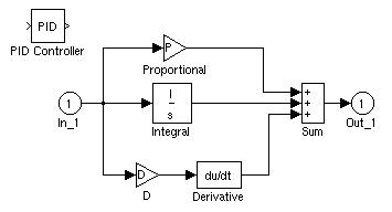
As for the two ready-made PID controllers, here's how they look like if you look under their masks:
 

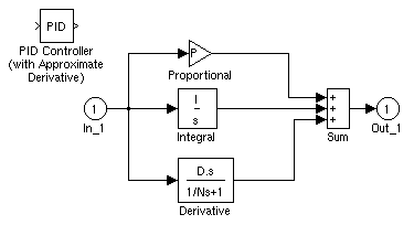The ideal PID controller function is P+I/s+Ds, and the "real" PID is P+I/s+Ds/(1/Ns+1). So P is the proportional gain Kc, I is Kc/taui_I, and D is Kc*tau_D as in Equation (5-8c) of our text. And N is what write as 1/(alpha*tau_D).