


Introduction
Over the last few decades, social scientists have developed and applied a host of statistical methods to make valid causal inferences, known as the credibility revolution. This trend has focused primarily on internal validity—researchers seek to unbiasedly estimate causal effects within a study, without making strong assumptions. One of the most important long-standing methodological debates is about external validity—how scientists can generalize causal findings beyond a specific study.
Although concepts of external validity are widely discussed in the social sciences, there are few empirical applications where researchers explicitly incorporate external validity into the design or analysis. Only
 $ 11\% $
of all experimental studies and
$ 11\% $
of all experimental studies and
 $ 13\% $
of all observational causal studies published in the American Political Science Review from 2015 to 2019 contain a formal analysis of external validity in the main text, and none discuss conditions under which generalization is credible.Footnote
1 The lack of empirical approaches for external validity has remained, potentially because social science studies have diverse goals and concerns surrounding external validity, and yet, most existing methodologies have focused primarily on the subset of threats that are statistically more tractable. In many applications, important concerns about external validity receive no empirical evaluation.
$ 13\% $
of all observational causal studies published in the American Political Science Review from 2015 to 2019 contain a formal analysis of external validity in the main text, and none discuss conditions under which generalization is credible.Footnote
1 The lack of empirical approaches for external validity has remained, potentially because social science studies have diverse goals and concerns surrounding external validity, and yet, most existing methodologies have focused primarily on the subset of threats that are statistically more tractable. In many applications, important concerns about external validity receive no empirical evaluation.
In this article, we develop a framework and methodologies to improve empirical approaches for external validity. Building on the classical experimental design literature (Campbell and Stanley Reference Campbell and Stanley1963; Shadish, Cook, and Campbell Reference Shadish, Cook and Campbell2002), we begin by proposing a unified causal framework that decomposes external validity into four components:
 $ X $
-,
$ X $
-,
 $ T $
-,
$ T $
-,
 $ Y $
-, and
$ Y $
-, and
 $ C $
-validity (populations, treatments, outcomes, and contexts/settings) in the section Formal Framework for External Validity. With the proposed framework, we formally synthesize a variety of external validity concerns researchers face in practice and relate them to causal assumptions—to name a few examples—convenience samples (
$ C $
-validity (populations, treatments, outcomes, and contexts/settings) in the section Formal Framework for External Validity. With the proposed framework, we formally synthesize a variety of external validity concerns researchers face in practice and relate them to causal assumptions—to name a few examples—convenience samples (
 $ X $
-validity), differences in treatment implementations (
$ X $
-validity), differences in treatment implementations (
 $ T $
-validity), survey versus behavioral outcomes (
$ T $
-validity), survey versus behavioral outcomes (
 $ Y $
-validity), and differences in causal mechanisms across time, geography, and/or institutions (
$ Y $
-validity), and differences in causal mechanisms across time, geography, and/or institutions (
 $ C $
-validity). We clarify conditions under which analysts can and cannot account for each type of validity.
$ C $
-validity). We clarify conditions under which analysts can and cannot account for each type of validity.
After researchers identify the most relevant dimensions of external validity using our proposed framework, they can determine the goal of the external validity analysis: effect- or sign-generalization. Effect-generalization considers how to generalize the magnitude of causal effects, and sign-generalization attempts to assess whether the direction of causal effects is generalizable. The former goal is important when researchers want to generalize the substantive or policy effect of treatments. The latter is relevant when analysts wish to test substantive theories that have observable implications only on the direction of treatment effects but not on the exact magnitude. Sign-generalization is also sometimes a practical compromise when effect-generalization, which requires stronger assumptions, is not feasible.
To enable effect-generalization, we introduce three classes of estimators and clarify the assumptions required by each (in the section Effect-Generalization). Weighting-based estimators adjust for selection into experiments, outcome-based estimators control for treatment effect heterogeneity, and doubly robust estimators combine both to mitigate the risk of model misspecification.
In the section Sign-Generalization, we propose a new approach to sign-generalization. It is increasingly common to include variations in relevant dimensions of external validity at the design stage—for example, measuring multiple outcomes, treatments, contexts, and diverse populations within each study. We formalize this common practice as the design of purposive variations and discuss why and when it is effective for testing the generalizability of the sign of causal effects. By extending a partial conjunction test (Benjamini and Heller Reference Benjamini and Heller2008; Karmakar and Small Reference Karmakar and Small2020), we then propose a novel sign-generalization test that combines purposive variations to quantify the extent of external validity. Because the design of purposive variations is already common in practice, application of the sign-generalization test can provide formal measures of external validity while requiring little additional practical cost.
To focus on issues of external validity, we use three randomized experiments, covering field, survey, and lab experiments, as our motivating applications (in the section Motivating Empirical Applications). Using them, we illustrate how to implement our proposed methods and provide practical recommendations in the section Empirical Applications and Appendix C. All of our methods can be implemented via the companion R package evalid. Finally, in the section Discussion, we discuss several important extensions. First, although the primary concern in observational studies is about internal validity, external validity is equally important for experimental and observational studies (Westreich et al. Reference Westreich, Edwards, Lesko, Cole and Stuart2019). We discuss how to analyze the same four dimensions of external validity in observational studies. Second, we discuss how our proposed methods are related to and helpful for meta-analysis and recent efforts toward scientific replication of experiments, such as the EGAP Metaketa initiative.
Our contributions are threefold. First, we formalize all four dimensions of external validity within the potential outcomes framework (Neyman Reference Neyman1923; Rubin Reference Rubin1974). Existing causal methods using potential outcomes have focused primarily on changes in populations—that is,
 $ X $
-validity (Cole and Stuart Reference Cole and Stuart2010; Egami and Hartman Reference Egami and Hartman2021; Imai, King, and Stuart Reference Imai, King and Stuart2008). Although a typology of external validity and different research goals of generalization are not new and have been discussed in the classical experimental design literature (Campbell and Stanley Reference Campbell and Stanley1963; Shadish, Cook, and Campbell Reference Shadish, Cook and Campbell2002), this literature has focused on providing conceptual clarity and did not use a formal causal framework. We relate each type of validity to explicit causal assumptions, which enables us to develop statistical methods that researchers can use in practice for generalization. Second, for effect-generalization of
$ X $
-validity (Cole and Stuart Reference Cole and Stuart2010; Egami and Hartman Reference Egami and Hartman2021; Imai, King, and Stuart Reference Imai, King and Stuart2008). Although a typology of external validity and different research goals of generalization are not new and have been discussed in the classical experimental design literature (Campbell and Stanley Reference Campbell and Stanley1963; Shadish, Cook, and Campbell Reference Shadish, Cook and Campbell2002), this literature has focused on providing conceptual clarity and did not use a formal causal framework. We relate each type of validity to explicit causal assumptions, which enables us to develop statistical methods that researchers can use in practice for generalization. Second, for effect-generalization of
 $ X $
-validity, we build on a large existing literature (Dahabreh et al. Reference Dahabreh, Robertson, Tchetgen, Stuart and Hernán2019; Hartman et al. Reference Hartman, Grieve, Ramsahai and Sekhon2015; Kern et al. Reference Kern, Stuart, Hill and Green2016; Tipton Reference Tipton2013) and provide practical guidance. To account for changes in populations and contexts together—that is,
$ X $
-validity, we build on a large existing literature (Dahabreh et al. Reference Dahabreh, Robertson, Tchetgen, Stuart and Hernán2019; Hartman et al. Reference Hartman, Grieve, Ramsahai and Sekhon2015; Kern et al. Reference Kern, Stuart, Hill and Green2016; Tipton Reference Tipton2013) and provide practical guidance. To account for changes in populations and contexts together—that is,
 $ X $
- and
$ X $
- and
 $ C $
-validity, we use identification results from the causal diagram approach (Bareinboim and Pearl Reference Bareinboim and Pearl2016) and develop new estimators in the section Effect-Generalization. The third and main methodological contribution is to provide a formal approach to sign-generalization. Although this important goal has been informally and commonly discussed in practice, to our knowledge, no method has been available. Finally, our work is distinct from and complementary to a recent review paper by Findley, Kikuta, and Denly (Reference Findley, Kikuta and Denly2020). The main goal of their work is to review how to evaluate external validity and how to report such evaluation in papers. In contrast, our paper focuses on how to improve external validity by proposing concrete methods (e.g., estimators and tests) that researchers can use in practice to implement effect- or sign-generalization.
$ C $
-validity, we use identification results from the causal diagram approach (Bareinboim and Pearl Reference Bareinboim and Pearl2016) and develop new estimators in the section Effect-Generalization. The third and main methodological contribution is to provide a formal approach to sign-generalization. Although this important goal has been informally and commonly discussed in practice, to our knowledge, no method has been available. Finally, our work is distinct from and complementary to a recent review paper by Findley, Kikuta, and Denly (Reference Findley, Kikuta and Denly2020). The main goal of their work is to review how to evaluate external validity and how to report such evaluation in papers. In contrast, our paper focuses on how to improve external validity by proposing concrete methods (e.g., estimators and tests) that researchers can use in practice to implement effect- or sign-generalization.
Motivating Empirical Applications
Field Experiment: Reducing Transphobia
Prejudice can negatively affect social, political, and health outcomes of out-groups experiencing discrimination. Yet, the prevailing literature has found intergroup prejudices highly resistant to change. In a recent study, Broockman and Kalla (Reference Broockman and Kalla2016) use a field experiment to study whether and how much a door-to-door canvassing intervention can reduce prejudice against transgender people. It was conducted in Miami-Dade County, Florida, in 2015 among voters who answered a preexperiment baseline survey. They randomly assigned canvassers to either encourage voters to actively take the perspective of transgender people (perspective taking) or to have a placebo conversation with respondents. To measure attitudes toward transgender people as outcome variables, they recruited respondents to four waves of follow-up surveys. The original authors find that the intervention involving a single approximately 10-minute conversation substantially reduced transphobia, and the effects persisted for three months.
Survey Experiment: Partisan-Motivated Reasoning
Scholars have been interested in how citizens perceive reality in ways that reflect well on their party, called partisan-motivated reasoning. Extending this literature, Bisgaard (Reference Bisgaard2019) theorizes that partisans can acknowledge the same economic facts and yet they rationalize reality using partisan-motivated reasoning. Those who support an incumbent party engage in blame-avoidant (credit-seeking) reasoning in the face of negative (positive) economic information, and opposition supporters behave conversely. To test this theory, the original author ran a total of four survey experiments across two countries, the United States and Denmark, to investigate whether substantive findings are consistent across different contexts where credit attribution of economic performance behaves differently. In each experiment, he recruited representative samples of the voting-age population and then randomly assigned subjects to receive either positive or negative news about changes in GDP. He measured how respondents update their economic beliefs and how they attribute responsibility for the economic changes to a ruling party. Across four experiments, he finds support for his hypotheses.
Lab Experiment: Effect of Emotions on Dissent in Autocracy
Many authoritarian countries employ various frightening acts of repression to deter dissent. To disentangle the psychological foundations of this authoritarian repression strategy, Young (Reference Young2019) asks, “Does the emotion of fear play an important role in shaping citizens’ willingness to dissent in autocracy, and if so, how?” (140). She theorizes that fear makes citizens more pessimistic about the risk of repression and, consequently, less likely to engage in dissent. To test this theory, the original author conducted a lab experiment in Zimbabwe in 2015. She recruited a hard-to-reach population of 671 opposition supporters using a form of snowball sampling. The experimental treatment induced fear using an experimental psychology technique called the autobiographical emotional memory task (AEMT); at its core, an enumerator asks a respondent to describe a situation that makes her relaxed (control condition) or afraid (treatment condition). As outcome variables, she measured propensity to dissent with a host of hypothetical survey outcomes and real-world, low-stakes behavioral outcomes. She finds that fear negatively affects dissent decisions, particularly through pessimism about the probability that other opposition supporters will also engage in dissent.
Formal Framework for External Validity
In external validity analysis, we ask whether causal findings are generalizable to other (1) populations, (2) treatments, (3) outcomes, and (4) contexts (settings) of theoretical interest. We incorporate all four dimensions into the potential outcomes framework (Neyman Reference Neyman1923; Rubin Reference Rubin1974) by extending the classical experimental design literature (Shadish, Cook, and Campbell Reference Shadish, Cook and Campbell2002). We will refer to each aspect as
 $ X $
-,
$ X $
-,
 $ T $
-,
$ T $
-,
 $ Y $
-, and
$ Y $
-, and
 $ C $
-validity, where
$ C $
-validity, where
 $ X $
represents pretreatment covariates of populations,
$ X $
represents pretreatment covariates of populations,
 $ T $
treatments,
$ T $
treatments,
 $ Y $
outcomes, and
$ Y $
outcomes, and
 $ C $
contexts. We will use an experimental study as an example because it helps us focus on issues of external validity. We discuss observational studies in the subsection External Validity of Observational Studies.
$ C $
contexts. We will use an experimental study as an example because it helps us focus on issues of external validity. We discuss observational studies in the subsection External Validity of Observational Studies.
Setup
Consider a randomized experiment with a total of
 $ n $
units, each indexed by
$ n $
units, each indexed by
 $ i\in \left\{1,\dots, n\right\} $
. We use
$ i\in \left\{1,\dots, n\right\} $
. We use
 $ \mathcal{P} $
to denote this experimental sample, within which a treatment variable
$ \mathcal{P} $
to denote this experimental sample, within which a treatment variable
 $ {T}_i $
is randomly assigned to each respondent. For notational clarity, we focus on a binary treatment
$ {T}_i $
is randomly assigned to each respondent. For notational clarity, we focus on a binary treatment
 $ {T}_i\in \left\{0,1\right\}, $
but the same framework is applicable to categorical and continuous treatments with appropriate notational changes. Researchers measure outcome variable
$ {T}_i\in \left\{0,1\right\}, $
but the same framework is applicable to categorical and continuous treatments with appropriate notational changes. Researchers measure outcome variable
 $ {Y}_i $
. We use
$ {Y}_i $
. We use
 $ {C}_i $
to denote a context to which unit
$ {C}_i $
to denote a context to which unit
 $ i $
belongs. For example, the field experiment by Broockman and Kalla (Reference Broockman and Kalla2016) was conducted in Miami-Dade County in Florida in 2015, and
$ i $
belongs. For example, the field experiment by Broockman and Kalla (Reference Broockman and Kalla2016) was conducted in Miami-Dade County in Florida in 2015, and
 $ {C}_i $
= (Miami, 2015).
$ {C}_i $
= (Miami, 2015).
We then define
 $ {Y}_i\left(T=t,c\right) $
to be the potential outcome variable of unit
$ {Y}_i\left(T=t,c\right) $
to be the potential outcome variable of unit
 $ i $
if the unit were to receive the treatment
$ i $
if the unit were to receive the treatment
 $ {T}_i=t $
within context
$ {T}_i=t $
within context
 $ {C}_i=c $
where
$ {C}_i=c $
where
 $ t\in \left\{0,1\right\} $
. In contrast to the standard potential outcomes, our framework explicitly shows that potential outcomes also depend on context
$ t\in \left\{0,1\right\} $
. In contrast to the standard potential outcomes, our framework explicitly shows that potential outcomes also depend on context
 $ C $
. This allows for the possibility that causal mechanisms of how the treatment affects the outcome can vary across contexts.
$ C $
. This allows for the possibility that causal mechanisms of how the treatment affects the outcome can vary across contexts.
Under the random assignment of the treatment variable
 $ T $
within the experiment, we can use simple estimators, such as difference-in-means, to estimate the sample average treatment effect (SATE).
$ T $
within the experiment, we can use simple estimators, such as difference-in-means, to estimate the sample average treatment effect (SATE).
 $$ \mathrm{SATE}\hskip0.35em \equiv \hskip0.35em {\unicode{x1D53C}}_{\mathcal{P}}\left\{{Y}_i\left(T\hskip0.35em =\hskip0.35em 1,c\right)-{Y}_i\left(T\hskip0.35em =\hskip0.35em 0,c\right)\right\}. $$
This represents the causal effect of treatment
 $ T $
on outcome
$ T $
on outcome
 $ Y $
for the experimental population
$ Y $
for the experimental population
 $ \mathcal{P} $
in context
$ \mathcal{P} $
in context
 $ C=c $
. The main issue of external validity is that researchers are interested not only in this within-experiment estimand but also whether causal conclusions are generalizable to other populations, treatments, outcomes, and contexts.
$ C=c $
. The main issue of external validity is that researchers are interested not only in this within-experiment estimand but also whether causal conclusions are generalizable to other populations, treatments, outcomes, and contexts.
We define the target population, treatment, outcome, and context to be the targets against which external validity of a given experiment is evaluated. These targets are defined by the goal of the researcher or policy maker. For example, Broockman and Kalla (Reference Broockman and Kalla2016) conducted an experiment with voluntary participants in Miami-Dade County in Florida. For
 $ X $
-validity, the target population could be adults in Miami, in Florida, in the US, or in any other populations of theoretical interest. The same question applies to other dimension—that is,
$ X $
-validity, the target population could be adults in Miami, in Florida, in the US, or in any other populations of theoretical interest. The same question applies to other dimension—that is,
 $ T $
-,
$ T $
-,
 $ Y $
-, and
$ Y $
-, and
 $ C $
-validity. Specifying targets is equivalent to clarifying studies’ scope conditions, and thus, this choice should be guided by substantive research questions and underlying theories of interest (Wilke and Humphreys Reference Wilke, Humphreys, Curini and Franzese2020).
$ C $
-validity. Specifying targets is equivalent to clarifying studies’ scope conditions, and thus, this choice should be guided by substantive research questions and underlying theories of interest (Wilke and Humphreys Reference Wilke, Humphreys, Curini and Franzese2020).
Formally, we define the target population average treatment effect (T-PATE) as follows:
 $$ \hskip-0.35em \mathrm{T}-\mathrm{PATE}\hskip0.35em \equiv \hskip0.35em {\unicode{x1D53C}}_{{\mathcal{P}}^{\ast }}\left\{{Y}_i^{\ast}\left({T}^{\ast}\hskip0.35em =\hskip0.35em 1,{c}^{\ast}\right)-{Y}_i^{\ast}\left({T}^{\ast}\hskip0.35em =\hskip0.35em 0,{c}^{\ast}\right)\right\}, $$
where * denotes the target of each dimension. Note that the methodological literature often defines the population average treatment effect by focusing only on the difference in populations
 $ \mathcal{P} $
and
$ \mathcal{P} $
and
 $ \mathcal{P} $
*, but our definition of the T-PATE explicitly considers all four dimensions.
$ \mathcal{P} $
*, but our definition of the T-PATE explicitly considers all four dimensions.
Therefore, we formalize a question of external validity as follows: Would we obtain the same causal conclusion (e.g., the magnitude or sign of causal effects) if we use the target population
 $ \mathcal{P} $
*, target treatment
$ \mathcal{P} $
*, target treatment
 $ {T}^{\ast } $
, target outcome
$ {T}^{\ast } $
, target outcome
 $ {Y}^{\ast } $
, and target context
$ {Y}^{\ast } $
, and target context
 $ {c}^{\ast } $
? Most importantly, external validity is defined with respect to specific targets researchers specify. This is essential because no experiment is universally externally valid; a completely different experiment should, of course, return a different result. Therefore, to empirically evaluate the external validity of experiments in a fair way, both analysts and evaluators should clarify the targets against which they evaluate experiments. If the primary goal of the experiment is theory testing, these targets can be abstract theoretical concepts (e.g., incentives). On the other hand, if the goal is to generate policy recommendations for a real-world intervention, these targets are often more concrete.
$ {c}^{\ast } $
? Most importantly, external validity is defined with respect to specific targets researchers specify. This is essential because no experiment is universally externally valid; a completely different experiment should, of course, return a different result. Therefore, to empirically evaluate the external validity of experiments in a fair way, both analysts and evaluators should clarify the targets against which they evaluate experiments. If the primary goal of the experiment is theory testing, these targets can be abstract theoretical concepts (e.g., incentives). On the other hand, if the goal is to generate policy recommendations for a real-world intervention, these targets are often more concrete.
Typology of External Validity
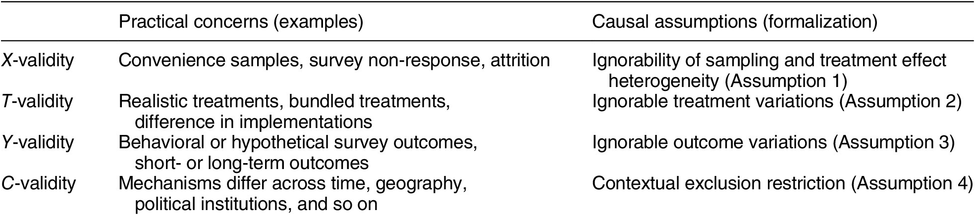
Building on a typology that has been influential conceptually (Campbell and Stanley Reference Campbell and Stanley1963), we provide a formal way to analyze practical concerns about external validity with the potential outcomes framework introduced in the previous section. We decompose external validity into four components,
 $ X $
-,
$ X $
-,
 $ T $
-,
$ T $
-,
 $ Y $
-, and
$ Y $
-, and
 $ C $
-validity, and we show how practical concerns in each dimension are related to fundamental causal assumptions. Table 1 previews a summary of the four dimensions.
$ C $
-validity, and we show how practical concerns in each dimension are related to fundamental causal assumptions. Table 1 previews a summary of the four dimensions.
Table 1. Summary of Typology
X-Validity
The difference in the composition of units in experimental samples and the target population is arguably the most well-known problem in the external validity literature (Imai, King, and Stuart Reference Imai, King and Stuart2008). When relying on convenience samples or nonprobability samples, such as undergraduate samples and online samples (e.g., Mechanical Turk and Lucid), many researchers worry that estimated causal effects for such samples may not generalize to other target populations.
Bias due to the difference between experimental sample
 $ \mathcal{P} $
and the target population
$ \mathcal{P} $
and the target population
 $ \mathcal{P} $
* can be addressed when selection into the experiment and treatment effect heterogeneity are unrelated to each other after controlling for pretreatment covariates
$ \mathcal{P} $
* can be addressed when selection into the experiment and treatment effect heterogeneity are unrelated to each other after controlling for pretreatment covariates
 $ \mathbf{X} $
(Cole and Stuart Reference Cole and Stuart2010).
$ \mathbf{X} $
(Cole and Stuart Reference Cole and Stuart2010).
Assumption 1 (Ignorability of Sampling and Treatment Effect Heterogeneity)
 $$ {Y}_i\left(T\hskip0.35em =\hskip0.35em 1,c\right)-{Y}_i\left(T\hskip0.35em =\hskip0.35em 0,c\right)\hskip2pt \perp \hskip-0.4em \perp \hskip2pt {S}_i\hskip0.2em \mid \hskip0.2em {\mathbf{X}}_i, $$
where
 $ {S}_i\in \left\{0,1\right\} $
indicates whether units are sampled into the experiment or not.
$ {S}_i\in \left\{0,1\right\} $
indicates whether units are sampled into the experiment or not.
The formal expression synthesizes two common approaches for addressing X-validity (Hartman Reference Hartman, Druckman and Green2020). The first approach attempts to account for how subjects are sampled into the experiment, including the common practice of using sampling weights (Miratrix et al. Reference Miratrix, Sekhon, Theodoridis and Campos2018; Mutz Reference Mutz2011). Random sampling is a well-known special case where no explicit sampling weights are required. The second common approach is based on treatment effect heterogeneity (e.g., Kern et al. Reference Kern, Stuart, Hill and Green2016). If analysts can adjust for all variables explaining treatment effect heterogeneity, Assumption 1 holds. A special case is when treatment effects are homogeneous: when true, the difference between the experimental sample and the target population does not matter and no adjustment is required. Relatedly, for some questions in survey experiments, recent studies find that causal estimates from convenience samples are similar to those estimated from nationally representative samples due to little treatment heterogeneity, despite the significant difference in their sample characteristics (Coppock, Leeper, and Mullinix Reference Coppock, Leeper and Mullinix2018; Mullinix et al. Reference Mullinix, Leeper, Druckman and Freese2015). Combining the two ideas, a general approach for X-validity is to adjust for variables that affect selection into an experiment and moderate treatment effects. The required assumption is violated when unobserved variables affect both sampling and treatment effect heterogeneity.
T-Validity
In social science experiments, due to various practical and ethical constraints, the treatment implemented within an experiment is not necessarily the same as the target treatment that researchers are interested in for generalization.
In field experiments, this concern often arises due to difference in implementations. For example, when scaling up the perspective-taking treatment developed in Broockman and Kalla (Reference Broockman and Kalla2016), researchers might not be able to partner with equally established LGBT organizations and to recruit canvassers of similar quality. Many field experiments have found that details of implementation have important effects on treatment effectiveness.
In survey experiments, analysts are often concerned with whether randomly assigned information is realistic and whether respondents process it as they would do in the real world. For instance, Bisgaard (Reference Bisgaard2019) designs treatments by mimicking the contents of newspaper articles that citizens would likely read in everyday life, which are the target treatments.
In lab experiments, this concern is often about bundled treatments. To test theoretical mechanisms, it is important to experimentally activate a specific mechanism. However, in practice, randomized treatments often act as a bundle, activating several mechanisms together. For instance, Young (Reference Young2019) acknowledges that “[a]lthough the AEMT [the treatment in her experiment] is one of the best existing ways to induce a specific targeted emotion, in practice it tends to induce a bundle of positive or negative emotions” (144). In this line of discussion, researchers view treatments that activate specific causal mechanisms as the target and consider an assigned treatment as a combination of multiple target treatments. The concern is that individual effects cannot be isolated because each target treatment is not separately randomized.
Although the target treatments differ depending on the types of experiments and corresponding research goals, the practical challenges discussed above can be formalized as concerns over the same causal assumption. Formally, bias due to concerns of
 $ T $
-validity is zero when the treatment variation is irrelevant to treatment effects.
$ T $
-validity is zero when the treatment variation is irrelevant to treatment effects.
Assumption 2 (Ignorable Treatment-Variations)
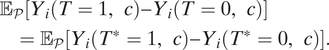 $$ {\displaystyle \begin{array}{l}{\unicode{x1D53C}}_{\mathcal{P}}\left[{Y}_i\left(T=1,c\right)-{Y}_i\left(T=0,c\right)\right]\\ {}\hskip1em ={\unicode{x1D53C}}_{\mathcal{P}}\left[{Y}_i\left({T}^{\ast }=1,c\right)-{Y}_i\left({T}^{\ast }=0,c\right)\right].\end{array}} $$
It states that the assigned treatment
 $ T $
and the target treatment
$ T $
and the target treatment
 $ {T}^{\ast } $
induce the same average treatment effects. For example, the causal effect of the perspective-taking intervention is the same regardless of whether canvassers are recruited by established LGBT organizations.
$ {T}^{\ast } $
induce the same average treatment effects. For example, the causal effect of the perspective-taking intervention is the same regardless of whether canvassers are recruited by established LGBT organizations.
Most importantly, a variety of practical concerns outlined above are about potential violations of this same assumption. Thus, we develop a general method—a new sign-generalization test in the section Sign-Generalization—that is applicable to concerns about T-validity regardless of whether they arise in field, survey, or lab experiments.
Y-Validity
Concerns of
 $ Y $
-validity arise when researchers cannot measure the target outcome in experiments. For example, in her lab experiment, Young (Reference Young2019) could not measure actual dissent behaviors, such as attending opposition meetings, for ethical and practical reasons. Instead, she relies on a low-risk behavioral measure of dissent (wearing a wristband with a pro-democracy slogan) and a host of hypothetical survey measures that span a range of risk levels.
$ Y $
-validity arise when researchers cannot measure the target outcome in experiments. For example, in her lab experiment, Young (Reference Young2019) could not measure actual dissent behaviors, such as attending opposition meetings, for ethical and practical reasons. Instead, she relies on a low-risk behavioral measure of dissent (wearing a wristband with a pro-democracy slogan) and a host of hypothetical survey measures that span a range of risk levels.
Similarly, in many experiments, even when researchers are inherently interested in behavioral outcomes, they often need to use hypothetical survey-based outcome measures—for example, support for hypothetical immigrants, policies, and politicians. In such cases,
 $ Y $
-validity analyses might ask whether causal effects learned with these hypothetical survey outcomes are informative about causal effects on the support for immigrants, policies, and politicians in the real world.
$ Y $
-validity analyses might ask whether causal effects learned with these hypothetical survey outcomes are informative about causal effects on the support for immigrants, policies, and politicians in the real world.
The difference between short-term and long-term outcomes is also related to
 $ Y $
-validity. In many social science experiments, researchers can only measure short-term outcomes and not the long-term outcomes of main interest.
$ Y $
-validity. In many social science experiments, researchers can only measure short-term outcomes and not the long-term outcomes of main interest.
Formally, a central question is whether outcome measures used in an experimental study are informative about the target outcomes of interest. Bias due to the difference in an outcome measured in the experiment
 $ Y $
and the target outcome
$ Y $
and the target outcome
 $ {Y}^{\ast } $
is zero when the outcome variation is irrelevant to treatment effects.
$ {Y}^{\ast } $
is zero when the outcome variation is irrelevant to treatment effects.
Assumption 3 (Ignorable Outcome Variations)
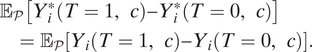 $$ {\displaystyle \begin{array}{l}{\unicode{x1D53C}}_{\mathcal{P}}\left[{Y}_i^{\ast}\left(T=1,c\right)-{Y}_i^{\ast}\left(T=0,c\right)\right]\\ {}\hskip1em ={\unicode{x1D53C}}_{\mathcal{P}}\left[{Y}_i\left(T=1,c\right)-{Y}_i\left(T=0,c\right)\right].\end{array}} $$
This assumption substantively means that the average causal effects are the same for outcomes measured in the experiment
 $ Y $
and for the target outcomes
$ Y $
and for the target outcomes
 $ {Y}^{\ast } $
. The assumption naturally holds if researchers measure the target outcome in the experiment—that is,
$ {Y}^{\ast } $
. The assumption naturally holds if researchers measure the target outcome in the experiment—that is,
 $ Y={Y}^{\ast } $
. For example, many Get-Out-the-Vote experiments in the US satisfy this assumption by directly measuring voter turnout with administrative records (e.g., Gerber and Green Reference Gerber and Green2012).
$ Y={Y}^{\ast } $
. For example, many Get-Out-the-Vote experiments in the US satisfy this assumption by directly measuring voter turnout with administrative records (e.g., Gerber and Green Reference Gerber and Green2012).
Thus, when analyzing
 $ Y $
-validity, researchers should consider how causal effects on the target outcome relate to those estimated with outcome measures in experiments. In the section Sign-Generalization, we discuss how to address this common concern about Assumption 3 by using multiple outcome measures.
$ Y $
-validity, researchers should consider how causal effects on the target outcome relate to those estimated with outcome measures in experiments. In the section Sign-Generalization, we discuss how to address this common concern about Assumption 3 by using multiple outcome measures.
We note that there are many issues about measurement that are related to but different from Y-validity, such as measurement error, social desirability bias, and most importantly, construct validity. Following Morton and Williams (Reference Morton and Williams2010), we argue that high construct validity helps
 $ Y $
-validity, but it is not sufficient. This is because the target outcome is often chosen based on theory, and thus, experiments with high construct validity are more likely to be externally valid in terms of outcomes. However, construct validity does not imply Y-validity. For example, as repeatedly found in the literature, practical differences in outcome measures (e.g., outcomes measured one year or two years after administration of a treatment) are often indistinguishable from a theoretical perspective, and yet they can induce large variation in treatment effects. We also provide further discussion on the relationship between external validity and other related concepts in Appendix G.
$ Y $
-validity, but it is not sufficient. This is because the target outcome is often chosen based on theory, and thus, experiments with high construct validity are more likely to be externally valid in terms of outcomes. However, construct validity does not imply Y-validity. For example, as repeatedly found in the literature, practical differences in outcome measures (e.g., outcomes measured one year or two years after administration of a treatment) are often indistinguishable from a theoretical perspective, and yet they can induce large variation in treatment effects. We also provide further discussion on the relationship between external validity and other related concepts in Appendix G.
C-Validity
Do experimental results generalize from one context to another context? This issue of
 $ C $
-validity is often at the heart of debates in external validity analysis (e.g., Deaton and Cartwright Reference Deaton and Cartwright2018). Social scientists often discuss geography and time as important contexts. For example, researchers might be interested in understanding whether and how we can generalize Broockman and Kalla’s (Reference Broockman and Kalla2016) study from Miami in 2015 to another context, such as New York City in 2020. Establishing
$ C $
-validity is often at the heart of debates in external validity analysis (e.g., Deaton and Cartwright Reference Deaton and Cartwright2018). Social scientists often discuss geography and time as important contexts. For example, researchers might be interested in understanding whether and how we can generalize Broockman and Kalla’s (Reference Broockman and Kalla2016) study from Miami in 2015 to another context, such as New York City in 2020. Establishing
 $ C $
-validity is challenging because a randomized experiment is done in one context
$ C $
-validity is challenging because a randomized experiment is done in one context
 $ c $
and researchers need to generalize or transport experimental results to another context
$ c $
and researchers need to generalize or transport experimental results to another context
 $ {c}^{\ast } $
, where they did not run the experiment. Formally,
$ {c}^{\ast } $
, where they did not run the experiment. Formally,
 $ C $
-validity is a question about covariates that have no variation within an experiment.
$ C $
-validity is a question about covariates that have no variation within an experiment.
Even though this concern about contexts has a long history (Campbell and Stanley Reference Campbell and Stanley1963), to our knowledge, the first general formal analysis of
 $ C $
-validity is given by Bareinboim and Pearl (Reference Bareinboim and Pearl2016) using a causal graphical approach. Building on this emerging literature, we formalize
$ C $
-validity is given by Bareinboim and Pearl (Reference Bareinboim and Pearl2016) using a causal graphical approach. Building on this emerging literature, we formalize
 $ C $
-validity within the potential outcomes framework introduced in the subsection Setup.
$ C $
-validity within the potential outcomes framework introduced in the subsection Setup.
We define
 $ C $
-validity as a question about mechanisms; how do treatment effects on the same units change across contexts? For example, in Broockman and Kalla (Reference Broockman and Kalla2016), even the same person might be affected differently by the perspective-taking intervention depending on whether she lives in New York City in 2020 or in Miami in 2015. Formally,
$ C $
-validity as a question about mechanisms; how do treatment effects on the same units change across contexts? For example, in Broockman and Kalla (Reference Broockman and Kalla2016), even the same person might be affected differently by the perspective-taking intervention depending on whether she lives in New York City in 2020 or in Miami in 2015. Formally,
 $$ \underset{\mathrm{Causal}\ \mathrm{effect}\ \mathrm{for}\ \mathrm{unit}\hskip0.2em i\hskip0.2em \mathrm{in}\ \mathrm{context}\hskip0.2em c}{\underbrace{Y_i\left(T=1,c\right)-{Y}_i\left(T=0,c\right)}}\ne \underset{\mathrm{Causal}\ \mathrm{effect}\ \mathrm{for}\ \mathrm{unit}\hskip0.2em i\hskip0.2em \mathrm{in}\ \mathrm{context}\hskip0.2em {c}^{\ast }}{\underbrace{Y_i\left(T=1,{c}^{\ast}\right)-{Y}_i\left(T=0,{c}^{\ast}\right)}}. $$
In order to generalize experimental results to another unseen context, we need to account for variables related to mechanisms through which contexts affect outcomes and moderate treatment effects. We refer to such variables as context moderators. Specifically, researchers need to assume that contexts affect outcomes only through measured context moderators. This implies that the causal effect for a given unit will be the same regardless of contexts, as long as the values of the context moderators are the same. For example, in Broockman and Kalla (Reference Broockman and Kalla2016), the context moderator could be the number of transgender individuals living in each unit’s neighborhood. Then, analysts might assume that the causal effect for a given unit will be the same regardless of whether she lives in New York City in 2020 or in Miami in 2015, as long as we adjust for the number of transgender individuals living in her neighborhood.
We formalize this assumption as the contextual exclusion restriction (Assumption 4), which states that the context variable
 $ {C}_i $
has no direct causal effect on the outcome once fixing the context moderators.Footnote
2 This name reflects its similarity to the exclusion restriction well known in the instrumental variable literature.
$ {C}_i $
has no direct causal effect on the outcome once fixing the context moderators.Footnote
2 This name reflects its similarity to the exclusion restriction well known in the instrumental variable literature.
Assumption 4 (Contextual Exclusion Restriction)
 $$ {Y}_i\left(T=t,\boldsymbol{M}=\boldsymbol{m},c\right)={Y}_i\left(T=t,\boldsymbol{M}=\boldsymbol{m},{c}^{\ast}\right), $$
where the potential outcome
 $ {Y}_i\left(T=t,c\right) $
is expanded with the potential context moderators
$ {Y}_i\left(T=t,c\right) $
is expanded with the potential context moderators
 $ {\mathbf{M}}_i(c) $
as
$ {\mathbf{M}}_i(c) $
as
 $ {Y}_i\left(T=t,c\right)={Y}_i\left(T=t,{\mathbf{M}}_i(c),c\right) $
, and then,
$ {Y}_i\left(T=t,c\right)={Y}_i\left(T=t,{\mathbf{M}}_i(c),c\right) $
, and then,
 $ {\mathbf{M}}_i(c) $
is fixed to
$ {\mathbf{M}}_i(c) $
is fixed to
 $ \mathbf{m} $
. We define
$ \mathbf{m} $
. We define
 $ {\mathbf{M}}_i $
to be a vector of context moderators, and thus, researchers can incorporate any number of variables to satisfy the contextual exclusion restriction. See Appendix H.2 for the proof of the identification of the T-PATE under this contextual exclusion restriction and other standard identification assumptions.
$ {\mathbf{M}}_i $
to be a vector of context moderators, and thus, researchers can incorporate any number of variables to satisfy the contextual exclusion restriction. See Appendix H.2 for the proof of the identification of the T-PATE under this contextual exclusion restriction and other standard identification assumptions.
Most importantly, this assumption implies that the causal effect for a given unit will be the same regardless of contexts, as long as the values of the context moderators are the same. Formally,
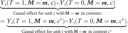 $$ \hskip1em {\displaystyle \begin{array}{l}\underset{\mathrm{Causal}\ \mathrm{effect}\ \mathrm{for}\ \mathrm{unit}\hskip0.2em i\hskip0.2em \mathrm{with}\;\mathbf{M}\hskip0.2em =\hskip0.2em \mathbf{m}\hskip0.33em \mathrm{in}\ \mathrm{context}\; c}{\underbrace{Y_i\left(T=1,\boldsymbol{M}=\boldsymbol{m},c\right)-{Y}_i\left(T=0,\boldsymbol{M}=\boldsymbol{m},c\right)}}\\ {}=\underset{\mathrm{Causal}\ \mathrm{effect}\ \mathrm{for}\ \mathrm{unit}\hskip0.2em i\hskip0.2em \mathrm{with}\;\mathbf{M} = \boldsymbol{m}\hskip0.33em \mathrm{in}\ \mathrm{context}\hskip0.2em {c}^{\ast }}{\underbrace{Y_i\left(T=1,\boldsymbol{M}=\boldsymbol{m},{c}^{\ast}\right)-{Y}_i\left(T=0,\boldsymbol{M}=\boldsymbol{m},{c}^{\ast}\right)}}.\end{array}} $$
This assumption is plausible when the measured context moderators capture all the reasons why causal effects vary across contexts. In other words, after conditioning on measured context moderators, there is no remaining context-level treatment effect heterogeneity. In contrast, if there are other channels through which contexts affect outcomes and moderate treatment effects, the assumption is violated.
Several points about Assumption 4 are worth clarifying. First, there is no general randomization design that makes Assumption 4 true. This is similar to the case of instrumental variables in that the exclusion restriction needs justification based on domain knowledge even when instruments are randomized (Angrist, Imbens, and Rubin Reference Angrist, Imbens and Rubin1996). Second, in order to avoid posttreatment bias, context moderators
 $ {\mathbf{M}}_i $
cannot be affected by treatment
$ {\mathbf{M}}_i $
cannot be affected by treatment
 $ {T}_i $
. In Broockman and Kalla (Reference Broockman and Kalla2016), it is plausible that the door-to-door canvassing interventions do not affect the number of transgender people in one’s neighborhood, a context moderator.
$ {T}_i $
. In Broockman and Kalla (Reference Broockman and Kalla2016), it is plausible that the door-to-door canvassing interventions do not affect the number of transgender people in one’s neighborhood, a context moderator.
Finally, we clarify the subtle yet important difference between
 $ X $
- and
$ X $
- and
 $ C $
-validity. Most importantly, the same variables may be considered as issues of
$ C $
-validity. Most importantly, the same variables may be considered as issues of
 $ X $
- or
$ X $
- or
 $ C $
-validity depending on the nature of the problem and data at hand. The main question is whether the variable has any variation within an experiment—if the variable has some variation, it is an
$ C $
-validity depending on the nature of the problem and data at hand. The main question is whether the variable has any variation within an experiment—if the variable has some variation, it is an
 $ X $
-validity problem, and it is a C-validity problem otherwise. For example, suppose we conduct a Get-Out-The-Vote experiment in an electorally safe district in Florida. If we want to generalize this experimental result to another district in Florida that is electorally competitive, the competitiveness in the district is a question about
$ X $
-validity problem, and it is a C-validity problem otherwise. For example, suppose we conduct a Get-Out-The-Vote experiment in an electorally safe district in Florida. If we want to generalize this experimental result to another district in Florida that is electorally competitive, the competitiveness in the district is a question about
 $ C $
-validity. This is because our experimental data does not contain any data from an electorally competitive district, which defines the target context. However, suppose we conduct a statewide experiment in Florida where some districts are electorally competitive and others are safe. Then, if we want to generalize this result to another state—for example, the state of New York—where the proportion of electorally competitive districts differs, the electoral competitiveness of districts can be addressed as an X-validity problem.Footnote
3 This is because our experimental data has both electorally competitive and safe districts and what differs across the two states is their distribution. In general,
$ C $
-validity. This is because our experimental data does not contain any data from an electorally competitive district, which defines the target context. However, suppose we conduct a statewide experiment in Florida where some districts are electorally competitive and others are safe. Then, if we want to generalize this result to another state—for example, the state of New York—where the proportion of electorally competitive districts differs, the electoral competitiveness of districts can be addressed as an X-validity problem.Footnote
3 This is because our experimental data has both electorally competitive and safe districts and what differs across the two states is their distribution. In general,
 $ X $
-validity is a question about the representativeness of the experimental data. Thus, X-validity is of primary concern when we ask whether the distribution of certain variables in the experiment is similar to the target population distribution of the same variables. In contrast,
$ X $
-validity is a question about the representativeness of the experimental data. Thus, X-validity is of primary concern when we ask whether the distribution of certain variables in the experiment is similar to the target population distribution of the same variables. In contrast,
 $ C $
-validity is a question about transportation (Bareinboim and Pearl Reference Bareinboim and Pearl2016) to a new context. Thus,
$ C $
-validity is a question about transportation (Bareinboim and Pearl Reference Bareinboim and Pearl2016) to a new context. Thus,
 $ C $
-validity is the main concern when we ask whether the experimental result is generalizable to a context where no experimental data exist.
$ C $
-validity is the main concern when we ask whether the experimental result is generalizable to a context where no experimental data exist.
The Proposed Approach to External Validity: Outline
In the section Formal Framework for External Validity, we developed a formal framework and discussed concerns for external validity. In this section, we outline our proposed approach to external validity, reserving details of our methods to the sections Effect-Generalization and Sign-Generalization.
The first step of external validity analysis is to ask which dimensions of external validity are most relevant in one’s application. For example, in the field experiment by Broockman and Kalla (Reference Broockman and Kalla2016), we focus primarily on
 $ X $
-validity (their experimental sample was restricted to Miami-Dade registered voters who responded to a baseline survey) and
$ X $
-validity (their experimental sample was restricted to Miami-Dade registered voters who responded to a baseline survey) and
 $ Y $
-validity (the original authors are interested in effects on both short- and long-term outcomes), whereas we discuss all four dimensions in Appendix C. We also provide additional examples of how to identify relevant dimensions in the section Empirical Applications and Appendix C. Regardless of the type of experiment, researchers should consider all four dimensions of external validity and identify relevant ones. We refer readers to the section Formal Framework for External Validity on the specifics of how to conceptualize each dimension.
$ Y $
-validity (the original authors are interested in effects on both short- and long-term outcomes), whereas we discuss all four dimensions in Appendix C. We also provide additional examples of how to identify relevant dimensions in the section Empirical Applications and Appendix C. Regardless of the type of experiment, researchers should consider all four dimensions of external validity and identify relevant ones. We refer readers to the section Formal Framework for External Validity on the specifics of how to conceptualize each dimension.
Once relevant dimensions are identified, analysts should decide the goal of an external validity analysis, whether effect- or sign-generalization. Effect-Generalization—generalizing the magnitude of the causal effect—is a central concern for randomized experiments that have policy implications. For example, in the field experiment by Broockman and Kalla (Reference Broockman and Kalla2016), effect-generalization is essential because cost–benefit considerations will be affected by the actual effect size. Sign-generalization—evaluating whether the sign of causal effects is generalizable—is relevant when researchers are testing theoretical mechanisms and substantive theories have observable implications on the direction or the order of treatment effects but not on the effect magnitude. For example, our motivating examples of Bisgaard (Reference Bisgaard2019) and Young (Reference Young2019) explicitly write main hypotheses in terms of the sign of causal effects.
Given the goal, the next step is to ask whether the specified goal is achievable by evaluating the assumptions required for each goal in relevant external validity dimensions. The assumptions required for effect-generalization include Assumptions 1–4 detailed in the section Formal Framework for External Validity, whereas we describe assumptions necessary for sign-generalization in the section Sign-Generalization. In some settings, researchers can design experiments such that the required assumptions are plausible, which is often the preferred approach. Importantly, even if effect-generalization is infeasible, sign-generalization might be possible in a wide range of applications, as it requires much weaker assumptions. Thus, sign-generalization is also sometimes a practical compromise when effect-generalization is not feasible.
We emphasize that, even if external validity concerns are acute, credible effect- or sign-generalization might be impossible given the design of the experiment, available data, and the nature of the problem. In such cases, we recommend that researchers clarify which dimensions of external validity are most concerning and why effect- and sign-generalization are not possible (e.g., required assumptions are untenable, or required data on target populations, treatments, outcomes, or contexts are not available).
In the sections Effect-Generalization and Sign-Generalization, we discuss how to conduct effect- and sign-generalization, respectively, when researchers can credibly justify the required assumptions. Our proposed workflow is summarized in Figure 1, and we refer readers there for a holistic view of our approach to external validity in practice.
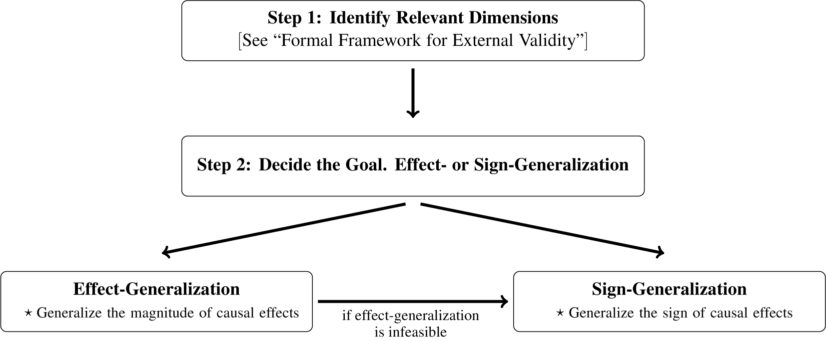
Figure 1. The Proposed Approach to External Validity
Effect-Generalization
In this section, we discuss how to conduct effect-generalization—including how to identify and estimate the T-PATE. This goal is most relevant for randomized experiments that seek to make policy recommendations. To keep the exposition clear, we first consider each dimension separately to highlight the difference in required assumptions and available solutions (we discuss how to address multiple dimensions together in the subsection Addressing Multiple Dimensions Together).
For X- and
 $ C $
-validity, we start by asking whether effect-generalization is feasible by evaluating the required assumptions (Assumption 1 for X-validity, and Assumption 4 for C-validity). If the required assumptions hold, researchers can employ three classes of estimators—weighting-based, outcome-based, and doubly robust estimators. We provide practical guidance on how to choose an estimator in the subsection How to Choose a T-PATE Estimator. Importantly, because the required assumptions are often strong, credible effect-generalization might be impossible. In such cases, sign-generalization might still be feasible because it requires weaker assumptions (see the section Sign-Generalization).
$ C $
-validity, we start by asking whether effect-generalization is feasible by evaluating the required assumptions (Assumption 1 for X-validity, and Assumption 4 for C-validity). If the required assumptions hold, researchers can employ three classes of estimators—weighting-based, outcome-based, and doubly robust estimators. We provide practical guidance on how to choose an estimator in the subsection How to Choose a T-PATE Estimator. Importantly, because the required assumptions are often strong, credible effect-generalization might be impossible. In such cases, sign-generalization might still be feasible because it requires weaker assumptions (see the section Sign-Generalization).
For
 $ T $
- and
$ T $
- and
 $ Y $
-validity, we argue the required assumptions are much more difficult to justify after experiments are completed. Therefore, we emphasize the importance of designing experiments such that their required assumptions (Assumptions 2 and 3) are plausible by designing treatments and measuring outcomes as similar as possible to their targets. We also highlight in the section Sign-Generalization that sign-generalization is more appropriate for addressing T- and Y-validity when researchers cannot modify their experiment to satisfy the required assumptions.
$ Y $
-validity, we argue the required assumptions are much more difficult to justify after experiments are completed. Therefore, we emphasize the importance of designing experiments such that their required assumptions (Assumptions 2 and 3) are plausible by designing treatments and measuring outcomes as similar as possible to their targets. We also highlight in the section Sign-Generalization that sign-generalization is more appropriate for addressing T- and Y-validity when researchers cannot modify their experiment to satisfy the required assumptions.
Our proposed approach is summarized in Figure 2, separately for
 $ X $
- and
$ X $
- and
 $ C $
-validity and
$ C $
-validity and
 $ T $
- and
$ T $
- and
 $ Y $
-validity.
$ Y $
-validity.

Figure 2. Summary of Effect-Generalization
X-Validity: Three Classes of Estimators
Researchers need to adjust for differences between experimental samples and the target population to address
 $ X $
-validity (Assumption 1). We provide formal definitions of estimators and technical details in Appendix H.2.
$ X $
-validity (Assumption 1). We provide formal definitions of estimators and technical details in Appendix H.2.
Weighting-Based Estimator
The first is a weighting-based estimator. The basic idea is to estimate the probability that units are sampled into the experiment, which is then used to weight experimental samples to approximate the target population. A common example is the use of survey weights in survey experiments.
Two widely-used estimators in this class are (1) an inverse probability weighted (IPW) estimator (Cole and Stuart Reference Cole and Stuart2010) and (2) an ordinary least squares estimator with sampling weights (weighted OLS). Without weights, these estimators are commonly used for estimating the SATE—that is, causal effects within the experiment. When incorporating sampling weights, these estimators are consistent for the T-PATE under Assumption 1. Both estimators also require a modeling assumption that the sampling weights are correctly specified.
Outcome-Based Estimator
Although the weighting-based estimator focuses on the sampling process, we can also adjust for treatment effect heterogeneity to estimate the T-PATE (e.g., Kern et al. Reference Kern, Stuart, Hill and Green2016). A general two-step estimator is as follows. First, we estimate outcome models for the treatment and control groups, separately, in the experimental data. In the second step, we use the estimated models to predict potential outcomes for the target population data.
Formally, in the first step, we estimate the outcome model
 $ {\hat{g}}_t\left({\mathbf{X}}_i\right)\equiv \hat{\unicode{x1D53C}}\left({Y}_i|{T}_i=t,{\mathbf{X}}_i,{S}_i=1\right) $
for
$ {\hat{g}}_t\left({\mathbf{X}}_i\right)\equiv \hat{\unicode{x1D53C}}\left({Y}_i|{T}_i=t,{\mathbf{X}}_i,{S}_i=1\right) $
for
 $ t\in \left\{0,1\right\} $
, where
$ t\in \left\{0,1\right\} $
, where
 $ {S}_i=1 $
indicates an experimental unit. This outcome model can be as simple as ordinary least squares or rely on more flexible estimators. In the second step, for unit
$ {S}_i=1 $
indicates an experimental unit. This outcome model can be as simple as ordinary least squares or rely on more flexible estimators. In the second step, for unit
 $ j $
in the target population data
$ j $
in the target population data
 $ \mathcal{P} $
*, we predict its potential outcome
$ \mathcal{P} $
*, we predict its potential outcome
 $ {\hat{Y}}_j(t)={\hat{g}}_t\left({\mathbf{X}}_j\right) $
, and thus,
$ {\hat{Y}}_j(t)={\hat{g}}_t\left({\mathbf{X}}_j\right) $
, and thus,
 $ \hat{T\hbox{--} {PATE}_{OUT}}=\frac{1}{N}\;{\sum}_{j\in {\mathcal{P}}^{\ast }}({\hat{Y}}_j(1)-{\hat{Y}}_j(0)) $
, where the sum is over the target population data
$ \hat{T\hbox{--} {PATE}_{OUT}}=\frac{1}{N}\;{\sum}_{j\in {\mathcal{P}}^{\ast }}({\hat{Y}}_j(1)-{\hat{Y}}_j(0)) $
, where the sum is over the target population data
 $ \mathcal{P} $
*, and
$ \mathcal{P} $
*, and
 $ N $
is the size of the target population data.
$ N $
is the size of the target population data.
It is worth reemphasizing that this estimator requires Assumption 1 for identification of the T-PATE, and it also assumes that the outcome models are correctly specified.
Doubly Robust Estimator
Finally, we discuss a class of doubly robust estimators, which reduces the risk of model misspecification common in the first two approaches (Dahabreh et al. Reference Dahabreh, Robertson, Tchetgen, Stuart and Hernán2019; Robins, Rotnitzky, and Zhao Reference Robins, Rotnitzky and Zhao1994). Specifically, to use weighting-based estimators, we have to assume the sampling model is correctly specified (the pink area in Figure 3a). Similarly, outcome-based estimators assume the correct outcome model (the orange area). In contrast, doubly robust estimators are consistent for the T-PATE as long as either the outcome model or the sampling model is correctly specified; furthermore, analysts need not know which one is, in fact, correct. Figure 3b shows that the doubly robust estimator is consistent in much wider applications (the gray area in Figure 3b). Therefore, this estimator significantly relaxes the modeling assumptions of the previous two methods. Although they weaken the modeling assumptions, we restate that doubly robust estimators also require Assumption 1 for the identification of the T-PATE.
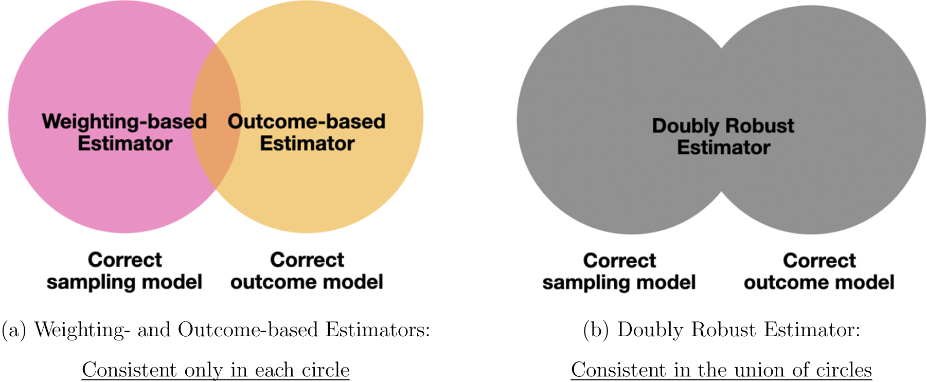
Figure 3. Properties of Doubly Robust Estimator
Note: The doubly robust estimator is consistent as long as the sampling or outcome model is correctly specified (gray area in panel b).
We now introduce the augmented IPW estimator (AIPW) in this class (Dahabreh et al. Reference Dahabreh, Robertson, Tchetgen, Stuart and Hernán2019; Robins, Rotnitzky, and Zhao Reference Robins, Rotnitzky and Zhao1994), which synthesizes the weighting-based and outcome-based estimators we discussed so far.
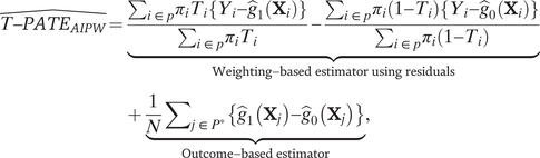 $$ \hat{T\hbox{--} {PATE}_{AIPW}}\hskip-0.2em =\hskip-0.2em {\displaystyle \begin{array}{l}\underset{\mathrm{Weighting}-\mathrm{based}\ \mathrm{estimator}\ \mathrm{using}\ \mathrm{residuals}}{\underbrace{\frac{\sum_{i\in p}{\pi}_i{T}_i\left\{{Y}_i-{\hat{g}}_1\left({\mathbf{X}}_i\right)\right\}}{\sum_{i\in p}{\pi}_i{T}_i}-\frac{\sum_{i\in p}{\pi}_i\left(1-{T}_i\right)\left\{{Y}_i-{\hat{g}}_0\left({\mathbf{X}}_i\right)\right\}}{\sum_{i\in p}{\pi}_i\left(1-{T}_i\right)}}}\\ {}+\hskip2px \underset{\mathrm{Outcome}-\mathrm{based}\ \mathrm{estimator}}{\underbrace{\frac{1}{N}{\sum}_{j\in {P}^{\ast }}\left\{{\hat{g}}_1\left({\mathbf{X}}_j\right)-{\hat{g}}_0\left({\mathbf{X}}_j\right)\right\}}},\end{array}} $$
where
 $ {\pi}_i $
is the sampling weight of unit
$ {\pi}_i $
is the sampling weight of unit
 $ i $
, and
$ i $
, and
 $ {\hat{g}}_t\left(\cdot \right) $
is an outcome model estimated in the experimental data. The first two terms represent the IPW estimator based on residuals
$ {\hat{g}}_t\left(\cdot \right) $
is an outcome model estimated in the experimental data. The first two terms represent the IPW estimator based on residuals
 $ {Y}_i-{\hat{g}}_t\left({\mathbf{X}}_i\right) $
, and the last term is equal to the outcome-based estimator.
$ {Y}_i-{\hat{g}}_t\left({\mathbf{X}}_i\right) $
, and the last term is equal to the outcome-based estimator.
How to Choose a T-PATE Estimator
In practice, researchers often do not know the true model for the sampling process (e.g., when using online panels or work platforms) or treatment effect heterogeneity. For this reason, we recommend doubly robust estimators to mitigate the risk of model misspecification whenever possible. However, there are scenarios when the alternative classes of estimators may be more appropriate. In particular, the weighted OLS can incorporate pretreatment covariates that are only measured in the experimental sample, which can greatly increase the precision in the estimation of the T-PATE (see the section Empirical Applications), while this estimator requires correctly specified sampling weights. As long as treatment effect heterogeneity is limited, the outcome-based estimator is also appropriate, especially when variance of sampling weights is large and the other two estimators tend to have large standard errors.
X- and C-Validity Together
In external validity analysis, concerns over X- and C-validity often arise together. This is because when we consider a target context different from the experimental context, both underlying mechanisms and populations often differ. To account for X- and
 $ C $
-validity together, we propose new estimators by generalizing sampling weights
$ C $
-validity together, we propose new estimators by generalizing sampling weights
 $ {\pi}_i\times {\theta}_i $
and outcome models
$ {\pi}_i\times {\theta}_i $
and outcome models
 $ g\left(\cdot \right) $
.
$ g\left(\cdot \right) $
.
 $$ {\hat{\pi}}_i\equiv \hskip-0.7em \underset{\begin{array}{c}\mathrm{Conditional}\ \mathrm{sampling}\ \mathrm{weights}\end{array}}{\underbrace{\frac{1}{\hat{\mathrm{Pr}\;}\;\left({S}_i=1|{C}_i=c,{\mathbf{M}}_i,{\mathbf{X}}_i\right)}}}\hskip-1em ,\hskip0.32em \mathrm{and}\hskip0.32em {\hat{\theta}}_i\equiv \hskip-2.8em \underset{\begin{array}{c}\mathrm{Difference}\ \mathrm{in}\ \mathrm{the}\ \mathrm{distributions}\\ {}\mathrm{across}\ \mathrm{contexts}\end{array}}{\underbrace{\frac{\hat{\mathrm{Pr}\;}\left({C}_i={c}^{\ast }|{\mathbf{M}}_i,{\mathbf{X}}_i\right)}{\hat{\mathrm{Pr}\;}\left({C}_i=c|{\mathbf{M}}_i,{\mathbf{X}}_i\right)}}} $$
 $$ \hat{g_t}({\mathbf{X}}_i,\;{\mathbf{M}}_i)\equiv \hat{\unicode{x1D53C}}\hskip-1.32em \underset{\begin{array}{c}\mathrm{Outcome}\ \mathrm{model}\ \mathrm{using}\ \mathrm{both}\hskip0.35em {\mathbf{X}}_i\hskip0.35em \mathrm{and}\hskip0.35em {\mathbf{M}}_i\end{array}}{\underbrace{\left({Y}_i|{T}_i=t,{\mathbf{X}}_i,{\mathbf{M}}_i,{S}_i=1,{C}_i=c\right)}}\hskip-1.2em ,\hskip0.4em \mathrm{for}\hskip0.4em t\in \left\{0,1\right\}, $$
where
 $ {\mathbf{X}}_i $
are covariates necessary for Assumption 1 and
$ {\mathbf{X}}_i $
are covariates necessary for Assumption 1 and
 $ {\mathbf{M}}_i $
are context moderators necessary for Assumption 4.
$ {\mathbf{M}}_i $
are context moderators necessary for Assumption 4.
 $ {\hat{\pi}}_i $
is the same as sampling weights used for
$ {\hat{\pi}}_i $
is the same as sampling weights used for
 $ X $
-validity, but it should be multiplied by
$ X $
-validity, but it should be multiplied by
 $ {\hat{\theta}}_i $
, which captures the difference in the distribution of
$ {\hat{\theta}}_i $
, which captures the difference in the distribution of
 $ \left({\mathbf{X}}_i,{\mathbf{M}}_i\right) $
in the experimental context
$ \left({\mathbf{X}}_i,{\mathbf{M}}_i\right) $
in the experimental context
 $ c $
and the target context
$ c $
and the target context
 $ {c}^{\ast }. $
The outcome model
$ {c}^{\ast }. $
The outcome model
 $ {\hat{g}}_t\left(\cdot \right) $
uses both
$ {\hat{g}}_t\left(\cdot \right) $
uses both
 $ {\mathbf{X}}_i $
and
$ {\mathbf{X}}_i $
and
 $ {\mathbf{M}}_i $
to explain outcomes. Note that estimators for X-validity alone (discussed in the subsection X-Validity: Three Classes of Estimators) or for
$ {\mathbf{M}}_i $
to explain outcomes. Note that estimators for X-validity alone (discussed in the subsection X-Validity: Three Classes of Estimators) or for
 $ C $
-validity alone are special cases of this proposed estimator. We provide technical details and proofs in Appendix H.
$ C $
-validity alone are special cases of this proposed estimator. We provide technical details and proofs in Appendix H.
T- and Y-Validity
Issues of T- and Y-validity are even more difficult in practice, which is naturally reflected in the strong assumptions discussed in the section Formal Framework for External Validity (Assumptions 2 and 3). This inherent difficulty is expected because defining a treatment and an outcome are the most fundamental pieces of any substantive theory; they formally set up potential outcomes, and they are directly defined based on research questions.
Therefore, we emphasize the importance of designing experiments such that the required assumptions are plausible by designing treatments and measuring outcomes as similar as possible to their targets. For example, to improve
 $ T $
-validity, Broockman and Kalla (Reference Broockman and Kalla2016) studied door-to-door canvassing conversations that typical LGBT organizations can implement in a real-world setting. To safely measure outcomes as similar as possible to the actual dissent decisions in autocracy, Young (Reference Young2019) carefully measured real-world, low-stakes behavioral outcomes in addition to asking hypothetical survey outcomes. This design-based approach is essential because, if the required assumptions hold by the design of the experiment, no additional adjustment is required for T- and Y-validity in the analysis stage. If such design-based solutions are not available, there is no general approach to conducting effect-generalization for
$ T $
-validity, Broockman and Kalla (Reference Broockman and Kalla2016) studied door-to-door canvassing conversations that typical LGBT organizations can implement in a real-world setting. To safely measure outcomes as similar as possible to the actual dissent decisions in autocracy, Young (Reference Young2019) carefully measured real-world, low-stakes behavioral outcomes in addition to asking hypothetical survey outcomes. This design-based approach is essential because, if the required assumptions hold by the design of the experiment, no additional adjustment is required for T- and Y-validity in the analysis stage. If such design-based solutions are not available, there is no general approach to conducting effect-generalization for
 $ T $
- and
$ T $
- and
 $ Y $
-validity without making stringent assumptions.
$ Y $
-validity without making stringent assumptions.
Importantly, even when effect-generalization is infeasible, researchers can assess external validity by examining the question of sign-generalization under weaker assumptions, which we discuss in the next section.
Sign-Generalization
We now consider the second research goal in external validity analysis: sign-generalization—evaluating whether the sign of causal effects is generalizable. This goal is most relevant when researchers are testing theoretical mechanisms and substantive theories have observable implications on the direction or the order of treatment effects but not on the effect magnitude. Sign-generalization is also sometimes a practical compromise when effect-generalization is not feasible.
The first step of sign-generalization is to include variations in relevant external validity dimensions at the design stage of experiments. To address
 $ X $
-,
$ X $
-,
 $ T $
-,
$ T $
-,
 $ Y $
-, and
$ Y $
-, and
 $ C $
-validity, researchers can include diverse populations, multiple treatments, outcomes, and contexts into experiments, respectively. Incorporating such explicit variations has a long history and is already standard in practice. We formalize this common practice as the design of purposive variations and show what assumption is necessary for using such purposive variations for sign-generalization (in the subsection Design of Purposive Variations). The required range assumption (Assumption 5) is much weaker than are the assumptions required for effect-generalization.
$ C $
-validity, researchers can include diverse populations, multiple treatments, outcomes, and contexts into experiments, respectively. Incorporating such explicit variations has a long history and is already standard in practice. We formalize this common practice as the design of purposive variations and show what assumption is necessary for using such purposive variations for sign-generalization (in the subsection Design of Purposive Variations). The required range assumption (Assumption 5) is much weaker than are the assumptions required for effect-generalization.
If researchers can include purposive variations to satisfy the required assumption, the final step is to conduct a new sign-generalization test, which computes partial conjunction p-values (Benjamini and Heller Reference Benjamini and Heller2008). Using these adjusted p-values, researchers can assess the direction of the T-PATE while accounting for multiple comparisons correctly. We detail their practical implementation and describe how to interpret them in the subsection Sign-Generalization Test. The main advantage is that the same proposed approach is applicable to all four dimensions. Our proposed approach is summarized in Figure 4, reserving methodological details for below.
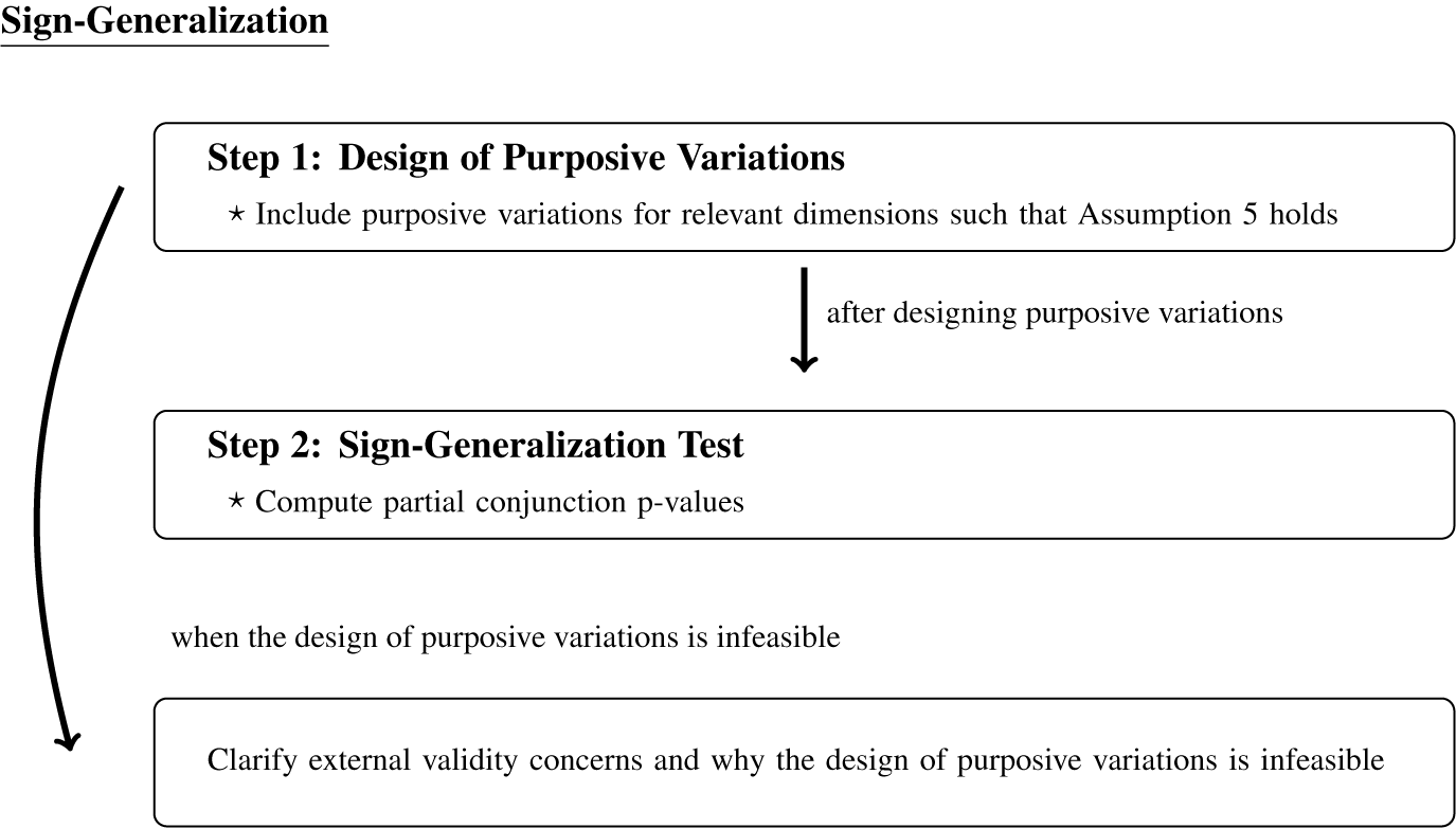
Figure 4. Summary of Sign-Generalization
Design of Purposive Variations
If possible, we woud like to test the sign of the T-PATE directly. However, it is infeasible in many applications because we often cannot observe target populations, treatments, outcomes, or contexts. Even in such scenarios, we can indirectly test the sign of the T-PATE by using multiple outcomes and incorporating diverse units, treatments, and contexts into experiments. The central idea is that if we consistently find positive (negative) causal effects across variations in all four dimensions, they together bolster evidence for a positive (negative) T-PATE (Shadish, Cook, and Campbell Reference Shadish, Cook and Campbell2002). We call this approach the design of purposive variations. Incorporating variations has a long history and is already standard in practice. In our review of all the experiments published in the APSR between 2015 and 2019, we found that more than 80% of articles included variations on at least one dimension.
Purposive variations are directly useful for showing the robustness of findings across the range of observed variations. However, without additional assumptions, the purposive variations are inherently local in that the variations are measured only within experiments, but by definition, external validity concerns are about variations we do not observe in the experiment. Therefore, we need to understand conditions under which purposive variations measured within the experiment help us infer the sign of the T-PATE, which is external to the experiment.
A practical question is “How should we incorporate purposive variations into experiments for testing the sign of the T-PATE?” To answer this, we now formally introduce the design of purposive variations. For the sake of clear presentation, we focus on
 $ Y $
-validity. We discuss other dimensions in the subsection Other Dimensions.
$ Y $
-validity. We discuss other dimensions in the subsection Other Dimensions.
Although there are many valid ways to choose variations for outcomes, we propose a simple approach based on a range.
Assumption 5 (Target Outcomes within a Range of Purposive Variations)
Choose
 $ K $
outcomes,
$ K $
outcomes,
 $ \left\{{Y}^1,\dots, {Y}^K\right\}, $
such that the T-PATE,
$ \left\{{Y}^1,\dots, {Y}^K\right\}, $
such that the T-PATE,
 $ {\unicode{x1D53C}}_{\mathcal{P}}\left\{{Y}_i^{\ast}\left(T=1,c\right)-{Y}_i^{\ast}\left(T=0,c\right)\right\} $
, is within a range of the
$ {\unicode{x1D53C}}_{\mathcal{P}}\left\{{Y}_i^{\ast}\left(T=1,c\right)-{Y}_i^{\ast}\left(T=0,c\right)\right\} $
, is within a range of the
 $ K $
causal effects
$ K $
causal effects
 $ {\left\{{\unicode{x1D53C}}_{\mathcal{P}}\left\{{Y}_i^k\left(T=1,c\right)-{Y}_i^k\left(T=0,c\right)\right\}\right\}}_{k=1}^K. $
Footnote
4
$ {\left\{{\unicode{x1D53C}}_{\mathcal{P}}\left\{{Y}_i^k\left(T=1,c\right)-{Y}_i^k\left(T=0,c\right)\right\}\right\}}_{k=1}^K. $
Footnote
4
Although this assumption might seem strong at first, its substantive meaning is natural. Intuitively, we choose the
 $ K $
outcomes such that the T-PATE is within a range of the
$ K $
outcomes such that the T-PATE is within a range of the
 $ K $
causal effects we estimate in the experiment (see Figure 5).
$ K $
causal effects we estimate in the experiment (see Figure 5).

Figure 5. Range Assumption
Without this assumption, inferences will heavily depend on extrapolation, which we wish to avoid. In practice, because we do not know the T-PATE, researchers can make this assumption more plausible by choosing a range of outcomes on which treatment effects are expected to be smaller and larger than the T-PATE. For example, Young (Reference Young2019) writes, “the items were selected to be contextually relevant and to span a range of risk levels” (145). Assumption 5 provides a formal justification for such a design of purposive variations.
This assumption is violated when the T-PATE is outside a range of causal effects covered by the
 $ K $
outcomes. For example, in Young (Reference Young2019), if the target outcome is a real-world high-risk dissent behavior and the intervention effect on this outcome is much smaller than those studied in the experiment, the range assumption is violated. At the same time, in this scenario no external validity analysis is possible without using extrapolation. Our proposed approach guards against such model-dependent extrapolation by clarifying underlying assumptions.
$ K $
outcomes. For example, in Young (Reference Young2019), if the target outcome is a real-world high-risk dissent behavior and the intervention effect on this outcome is much smaller than those studied in the experiment, the range assumption is violated. At the same time, in this scenario no external validity analysis is possible without using extrapolation. Our proposed approach guards against such model-dependent extrapolation by clarifying underlying assumptions.
Sign-Generalization Test
We now propose a new sign-generalization test. The goal here is to use purposive variations to test whether the sign of causal effects is generalizable.
Without loss of generality, suppose a substantive theory predicts that the T-PATE is positive. We focus again on
 $ Y $
-validity, and thus, our target null hypothesis can be written as
$ Y $
-validity, and thus, our target null hypothesis can be written as
 $$ {H}_0^{\ast }:{\unicode{x1D53C}}_{\mathcal{P}}\left\{{Y}_i^{\ast}\left(T=1,c\right)-{Y}_i^{\ast}\left(T=0,c\right)\right\}\hskip0.35em \le \hskip0.35em 0. $$
If we can provide statistical evidence against the null hypothesis
 $ {H}_0^{\ast } $
, we support the substantive theory predicting a positive effect.
$ {H}_0^{\ast } $
, we support the substantive theory predicting a positive effect.
When we cannot measure the target outcome
 $ {Y}^{\ast } $
in the experiment to directly evaluate this target hypothesis, we rely on the
$ {Y}^{\ast } $
in the experiment to directly evaluate this target hypothesis, we rely on the
 $ K $
hypotheses, corresponding to the
$ K $
hypotheses, corresponding to the
 $ K $
outcomes in experiments; for
$ K $
outcomes in experiments; for
 $ k\in \left\{1,\dots, K\right\}, $
 $$ {H}_0^k:{\unicode{x1D53C}}_{\mathcal{P}}\left\{{Y}_i^k\left(T=1,c\right)-{Y}_i^k\left(T=0,c\right)\right\}\hskip0.35em \le \hskip0.35em 0. $$
Connecting Purposive Variations to Sign-Generalization
We first show that when causal effects are positive (negative) for all
 $ K $
outcomes, the causal effect on the target outcome is also positive (negative) under the range assumption (Assumption 5). It implies that testing the union of the
$ K $
outcomes, the causal effect on the target outcome is also positive (negative) under the range assumption (Assumption 5). It implies that testing the union of the
 $ K $
null hypotheses (Equation 8) is a valid test for the target null hypothesis (Equation 7) under the range assumption. In practice, this means that a common approach of checking whether all
$ K $
null hypotheses (Equation 8) is a valid test for the target null hypothesis (Equation 7) under the range assumption. In practice, this means that a common approach of checking whether all
 $ K $
causal estimates are statistically significant at a prespecified significance level
$ K $
causal estimates are statistically significant at a prespecified significance level
 $ \alpha $
(e.g.,
$ \alpha $
(e.g.,
 $ \alpha =0.05\Big) $
is valid as a sign-generalization test, without additional multiple testing corrections (Berger and Hsu Reference Berger and Hsu1996). Details and derivations are presented in Appendix H.
$ \alpha =0.05\Big) $
is valid as a sign-generalization test, without additional multiple testing corrections (Berger and Hsu Reference Berger and Hsu1996). Details and derivations are presented in Appendix H.
Partial Conjunction Test
Although checking whether all p-values are smaller than
 $ \alpha $
is easy to implement, it can be too stringent in practice. For example, even if an estimated causal effect on just one out of many outcomes is not statistically significant, the method above is inconclusive about sign-generalization. However, intuitively, finding positive effects on most outcomes provides strong evidence for
$ \alpha $
is easy to implement, it can be too stringent in practice. For example, even if an estimated causal effect on just one out of many outcomes is not statistically significant, the method above is inconclusive about sign-generalization. However, intuitively, finding positive effects on most outcomes provides strong evidence for
 $ Y $
-validity.
$ Y $
-validity.
To incorporate such flexibility, we build on a formal framework of partial conjunction tests, which was recently formalized by Benjamini and Heller (Reference Benjamini and Heller2008) and extended to observational causal inference in Karmakar and Small (Reference Karmakar and Small2020). We extend the partial conjunction test framework to external validity analysis.
In the partial conjunction test, our goal is to provide evidence that the treatment has a positive effect on at least
 $ r $
out of
$ r $
out of
 $ K $
outcomes. Formally, the partial conjunction null hypothesis is as follows:
$ K $
outcomes. Formally, the partial conjunction null hypothesis is as follows:
 $$ {\overset{\sim }{H}}_0^r:\sum_{k=1}^K\hskip-0.3em \mathbf{1}\left\{{H}_0^k\hskip0.35em is\ false\right\}<r, $$
where
 $ r\hskip-0.1em \in \hskip-0.1em \left[1,K\right] $
is a threshold specified by researchers, and
$ r\hskip-0.1em \in \hskip-0.1em \left[1,K\right] $
is a threshold specified by researchers, and
 $ {\sum}_{k=1}^K\mathbf{1}\left\{{H}_0^k\hskip0.22em \mathrm{is}\ \mathrm{false}\hskip0.1em \right\} $
counts the number of true nonnulls. By rejecting this partial conjunction null, researchers can provide statistical evidence that the treatment has positive causal effects on at least
$ {\sum}_{k=1}^K\mathbf{1}\left\{{H}_0^k\hskip0.22em \mathrm{is}\ \mathrm{false}\hskip0.1em \right\} $
counts the number of true nonnulls. By rejecting this partial conjunction null, researchers can provide statistical evidence that the treatment has positive causal effects on at least
 $ r $
outcomes. For example, when
$ r $
outcomes. For example, when
 $ r=0.8K, $
researchers can assess whether the treatment has positive effects on at least
$ r=0.8K, $
researchers can assess whether the treatment has positive effects on at least
 $ 80\% $
of outcomes.
$ 80\% $
of outcomes.
How can we obtain a p-value for this partial conjunction test? We only need one-sided p-values computed separately for each of
 $ K $
outcomes
$ K $
outcomes
 $ \left\{{p}_1,\dots, {p}_K\right\} $
. We first sort them such that
$ \left\{{p}_1,\dots, {p}_K\right\} $
. We first sort them such that
 $ {p}_{(1)}\le \hskip0.35em {p}_{(2)}\le \dots \le \hskip0.35em {p}_{(K)}. $
Then, we define the partial conjunction p-values as follows:
$ {p}_{(1)}\le \hskip0.35em {p}_{(2)}\le \dots \le \hskip0.35em {p}_{(K)}. $
Then, we define the partial conjunction p-values as follows:
 $$ \hskip-14.9em {\tilde{p}}_{(1)}\equiv {Kp}_{(1)} $$
 $$ {\tilde{p}}_{(r)}\equiv \mathit{\max}\left\{\left(K-r+1\right){p}_{(r)},{\tilde{p}}_{\left(r-1\right)}\right\}\hskip0.2em \mathrm{for}\hskip0.35em r\ge 2. $$
The p-value for
 $ {\overset{\sim }{H}}_0^r $
is
$ {\overset{\sim }{H}}_0^r $
is
 $ \tilde{p}_{(r)} $
(see Figure 6 for an example). This procedure is valid under any dependence across p-values (see Appendix H.3). In Appendix H.3, we also discuss scenarios in which p-values are independent across variations.
$ \tilde{p}_{(r)} $
(see Figure 6 for an example). This procedure is valid under any dependence across p-values (see Appendix H.3). In Appendix H.3, we also discuss scenarios in which p-values are independent across variations.

Figure 6. Example of Partial Conjunction Test with Three Outcomes
Note: The second step of Correction is based on Equation 10.
Finally, it is important to emphasize that researchers do not need to specify the threshold r. Rather, we recommend reporting partial conjunction p-values
 $ \tilde{p}_{(r)} $
for every threshold
$ \tilde{p}_{(r)} $
for every threshold
 $ r $
(see Equation 10 and examples in the section Empirical Applications). For instance, in Figure 6, we would report all three partial conjunction p-values {0.03, 0.08, 0.08}, each testing whether at least 1, 2, or 3 out of our three outcomes have positive effects. Although researchers might be worried about a multiple testing problem, no further adjustment to p-values is required due to the monotonicity properties of the partial conjunction p-value (see Appendix H.3 and Benjamini and Heller Reference Benjamini and Heller2008). In addition, using the
$ r $
(see Equation 10 and examples in the section Empirical Applications). For instance, in Figure 6, we would report all three partial conjunction p-values {0.03, 0.08, 0.08}, each testing whether at least 1, 2, or 3 out of our three outcomes have positive effects. Although researchers might be worried about a multiple testing problem, no further adjustment to p-values is required due to the monotonicity properties of the partial conjunction p-value (see Appendix H.3 and Benjamini and Heller Reference Benjamini and Heller2008). In addition, using the
 $ K $
partial conjunction p-values, researchers can also directly estimate the number of outcomes for which the treatment has positive effects by counting the number of outcomes whose corresponding partial conjunction p values are less than
$ K $
partial conjunction p-values, researchers can also directly estimate the number of outcomes for which the treatment has positive effects by counting the number of outcomes whose corresponding partial conjunction p values are less than
 $ \alpha $
. For example, in Figure 6, the estimated number of outcomes that have positive effects is one because only one out of the three outcomes is significant at
$ \alpha $
. For example, in Figure 6, the estimated number of outcomes that have positive effects is one because only one out of the three outcomes is significant at
 $ \alpha =0.05 $
. We provide the details and proofs in Appendix H.3.
$ \alpha =0.05 $
. We provide the details and proofs in Appendix H.3.
Other Dimensions
Although this section focused on
 $ Y $
-validity for clear presentation, researchers can use the same sign-generalization test for other dimensions as long as purposive variations are included for each dimension of external validity. For purposive X-variations, researchers can explicitly sample distinct subgroups that they expect to have different treatment effects. For instance, in Broockman and Kalla (Reference Broockman and Kalla2016), researchers could explicitly recruit respondents who have transgender friends and those who do not. For purposive
$ Y $
-validity for clear presentation, researchers can use the same sign-generalization test for other dimensions as long as purposive variations are included for each dimension of external validity. For purposive X-variations, researchers can explicitly sample distinct subgroups that they expect to have different treatment effects. For instance, in Broockman and Kalla (Reference Broockman and Kalla2016), researchers could explicitly recruit respondents who have transgender friends and those who do not. For purposive
 $ T $
-variations, researchers can include treatment versions that change only one aspect at a time. For example, Young (Reference Young2019) induced fear in respondents with two versions of the treatment: “general fear condition” unrelated to politics and “political fear condition” directly related to politics. Finally, purposive C-variation is gaining popularity in political science. It has recently become more feasible to run survey experiments in multiple countries at multiple points (e.g., Bisgaard Reference Bisgaard2019), and an increasing number of researchers conduct multisite field experiments (e.g., Blair and McClendon Reference Blair, McClendon, Green and Druckman2020; Dunning et al. Reference Dunning, Grossman, Humphreys, Hyde, McIntos, Nellis and Adida2019). It is important to emphasize that researchers can also assess multiple dimensions together (e.g.,
$ T $
-variations, researchers can include treatment versions that change only one aspect at a time. For example, Young (Reference Young2019) induced fear in respondents with two versions of the treatment: “general fear condition” unrelated to politics and “political fear condition” directly related to politics. Finally, purposive C-variation is gaining popularity in political science. It has recently become more feasible to run survey experiments in multiple countries at multiple points (e.g., Bisgaard Reference Bisgaard2019), and an increasing number of researchers conduct multisite field experiments (e.g., Blair and McClendon Reference Blair, McClendon, Green and Druckman2020; Dunning et al. Reference Dunning, Grossman, Humphreys, Hyde, McIntos, Nellis and Adida2019). It is important to emphasize that researchers can also assess multiple dimensions together (e.g.,
 $ Y $
- and
$ Y $
- and
 $ T $
-validity together) with the same approach. We provide examples of doing so in the next section.
$ T $
-validity together) with the same approach. We provide examples of doing so in the next section.
Empirical Applications
We now report a reanalysis of Broockman and Kalla (Reference Broockman and Kalla2016) as an example of effect-generalization and Bisgaard (Reference Bisgaard2019) as an example of sign-generalization. In Appendix C, we provide results for Young (Reference Young2019), which focuses on sign-generalization.
Field Experiment: Reducing Transphobia
Broockman and Kalla (Reference Broockman and Kalla2016) find that a 10-minute perspective-taking conversation can lead to a durable reduction in transphobic beliefs. Typical of modern field experiments, their experimental sample was restricted to Miami-Dade registered voters who responded to a baseline survey, answered a face-to-face canvassing attempt, and responded to the subsequent survey waves, raising common concerns about X-validity. Unlike many other field experiments, their experiment provides a rare opportunity to evaluate Y-validity, in particular, whether the intervention has both short- and long-term effects, by measuring outcomes over time (three days, three weeks, six weeks, and three months after the intervention). For the main outcome variable, the original authors computed a single index in each wave based on a set of survey questions on attitudes toward transgender people. Given the significant policy implication of the effect magnitude, we study effect-generalization while addressing concerns of X- and Y-validity together. Given space constraints, we focus on these two dimensions, which are most insightful for illustrating the proposed approach, and we discuss T- and C-validity in Appendix C.1.
Although there are many potentially important target populations, we specify our target population to be all adults in Florida, defined using the common content data from the 2016 Cooperative Congressional Election Study (CCES).
To estimate the T-PATE, we adjust for age, sex, race/ethnicity, ideology, religiosity, and partisan identification, which include all variables measured in both the experiment and the CCES. Although these variables are similar to what applied researchers usually adjust for, we have to carefully assess the necessary identification assumption (Assumption 1). If unobserved variables, such as political interest, affect both sampling and effect heterogeneity, the assumption is untenable. Researchers can make this required assumption more plausible by measuring variables that affect both sampling and treatment effect heterogeneity.
Effect-Generalization
We estimate the T-PATE using the three classes of estimators discussed in the subsection X-Validity: Three Classes of Estimators. Weighting-based estimators include IPW and weighted OLS that adjust for control variables prespecified in the original authors’ preanalysis plan. Sampling weights are estimated via calibration (Hartman et al. Reference Hartman, Grieve, Ramsahai and Sekhon2015). For the outcome-based estimators, we use OLS and a more flexible model, Baysian additive regression trees (BART). Finally, we implement two doubly robust estimators; the augmented inverse probability weighted estimator (AIPW) with OLS and the AIPW with BART. We use block bootstrap to compute standard errors clustered at the household level as in the original study. All estimators are implemented by our companion R package evalid.
Figure 7 presents point estimates and their 95% confidence intervals using different estimators. Broockman and Kalla (Reference Broockman and Kalla2016) create an outcome index such that the value of one represents one standard deviation of the index outcome in the control group. Therefore, the estimated effects should be interpreted relative to outcomes in the control group. The first column shows estimates of the SATE for four periods, and the subsequent three columns present estimates of the T-PATE using the three classes of estimators from above.

Figure 7. Estimates of the T-PATE for Broockman and Kalla (Reference Broockman and Kalla2016)
Note: The first column shows estimates of the SATE, and the subsequent three columns present estimates of the T-PATE for three classes of estimators. Rows represent different posttreatment survey waves.
Several points are worth noting. First, the T-PATE estimates are similar to the SATE estimate, and this pattern is stable across all periods. By accounting for
 $ X $
- and Y-validity, this analysis suggests that Broockman and Kalla (Reference Broockman and Kalla2016)’s intervention has similar effects in the target population across all periods. We emphasize that, whereas the SATE estimate and the T-PATE estimates are similar in this application, bias in the SATE estimates can be large in many applications (see Appendix I for illustrations). Thus, we recommend estimating the T-PATE formally and comparing it against the SATE estimate.
$ X $
- and Y-validity, this analysis suggests that Broockman and Kalla (Reference Broockman and Kalla2016)’s intervention has similar effects in the target population across all periods. We emphasize that, whereas the SATE estimate and the T-PATE estimates are similar in this application, bias in the SATE estimates can be large in many applications (see Appendix I for illustrations). Thus, we recommend estimating the T-PATE formally and comparing it against the SATE estimate.
Second, in general, estimates of the T-PATE have larger standard errors compared with that of the SATE. This is natural and necessary because the estimation of the T-PATE must also account for differences between the experimental sample and the target population. Importantly, both the point estimate and the standard error of the T-PATE affect the cost–benefit analysis. Thus, even though point estimates are similar, the cost–benefit analysis for the target population has more uncertainty due to the larger standard error of the T-PATE.
Finally, we can compare the three classes of estimators. We generally recommend doubly robust estimators because the sampling and outcome models are often unknown in practice. However, in this example the weighted least squares estimator (wLS in Figure 7) also has a desirable feature; it is the most efficient estimator because it can incorporate many pretreatment covariates measured only in the experiment, whereas other estimators cannot. Note that this estimator assumes the correct specification of sampling weights. Outcome-based estimators are also effective here because there is limited treatment effect heterogeneity as found in the original article. Indeed, all estimators provide relatively stable T-PATE estimates, which are close to the SATE in this example. By following similar reasoning, researchers can determine an appropriate estimator in each application (see also the subsection How to Choose a T-PATE Estimator).
Survey Experiment: Partisan-Motivated Reasoning
Bisgaard (Reference Bisgaard2019) finds that, even when partisans agree on the facts, partisan-motivated reasoning influences how they internalize those facts and attribute credit (or blame) to incumbents. In terms of external validity analysis, Bisgaard (Reference Bisgaard2019) provides several great opportunities to evaluate sign-generalization in terms of
 $ C $
- and
$ C $
- and
 $ Y $
-validity. We discuss
$ Y $
-validity. We discuss
 $ X $
- and
$ X $
- and
 $ T $
-validity in Appendix C.2.
$ T $
-validity in Appendix C.2.
For
 $ C $
-validity, the study incorporates purposive variations by running a total of four survey experiments across two countries, the United States and Denmark (Study 1 in the US and Studies 2–4 in Denmark. See Table 1 of the original study for more details). They differ in terms of both political and economic settings; the incumbent party’s political responsibility for the economy is less clear, and the level of polarization among citizens is lower in Denmark than in the United States.
$ C $
-validity, the study incorporates purposive variations by running a total of four survey experiments across two countries, the United States and Denmark (Study 1 in the US and Studies 2–4 in Denmark. See Table 1 of the original study for more details). They differ in terms of both political and economic settings; the incumbent party’s political responsibility for the economy is less clear, and the level of polarization among citizens is lower in Denmark than in the United States.
Although generalization to a new target context was not a clear goal of the original paper, there are potentially many relevant target contexts. For example, Germany shares political and geographic features with Denmark and its global economic power with the United States. Thus, if researchers are interested in generalizing results to Germany, it may be reasonable to assume that the purposive contextual variations in Bisgaard (Reference Bisgaard2019) satisfy the required range assumption (Assumption 5).
In terms of Y-validity, to measure how citizens attribute responsibilities to incumbents, the original author uses three different sets of outcomes: closed-ended survey responses, open-ended-survey responses, and argument rating tasks. The target outcome is citizens’ attribution of responsibility to incumbents when they read economic news in everyday life. The three sets of outcomes provide reasonable variations to capture this target outcome by balancing specificity and reality. We assume that the three sets of outcomes jointly satisfy the required range assumption, and we use all the outcomes for the sign-generalization test.
Sign-Generalization Test
The theory of Bisgaard (Reference Bisgaard2019) can be summarized into two hypotheses, one for supporters of the incumbent party and the other for those of the opposition party. In the face of positive economic facts, supporters of the incumbent party will be more likely (H1) and supporters of the opposition party will be less likely (H2) to believe the incumbent party is responsible for the economy. We estimate the treatment effect of showing positive economic news on the attribution of responsibility relative to that of showing negative economic news. Thus, for supporters of the incumbent party, the first hypothesis (H1) predicts that the treatment effects are positive, and for supporters of the opposition party, the second hypothesis (H2) predicts that the treatment effects are negative.
For our external validity analysis, we test each hypothesis by considering
 $ C $
- and
$ C $
- and
 $ Y $
-validity together using the sign-generalization test. The combination of multiple outcomes across four survey experiments in two countries yields 12 causal estimates corresponding to each hypothesis (see Table 2). We then assess the proportion of positive causal effects for the first hypothesis and that of negative causal effects for the second hypothesis using the proposed partial conjunction test.
$ Y $
-validity together using the sign-generalization test. The combination of multiple outcomes across four survey experiments in two countries yields 12 causal estimates corresponding to each hypothesis (see Table 2). We then assess the proportion of positive causal effects for the first hypothesis and that of negative causal effects for the second hypothesis using the proposed partial conjunction test.
Table 2. Design of Purposive Variations for Bisgaard (Reference Bisgaard2019)
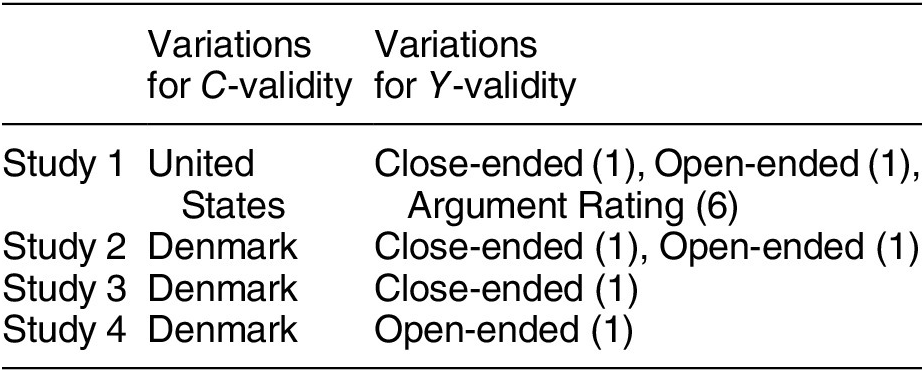
Note: The number of the purposive outcome variations is in parentheses.
For each hypothesis, Figure 8 presents results from the partial conjunction test for all thresholds. Each p-value is colored by context, with Denmark in red and the United States in blue. Variations in outcome are represented by symbols. For incumbent supporters, we find 8 out of 12 outcomes (
 $ 66\% $
) have partial conjunction p-values less than the conventional significance level of
$ 66\% $
) have partial conjunction p-values less than the conventional significance level of
 $ 0.05 $
. It is notable that most of the estimates that do not support the theory are from Denmark, which we might expect because partisan-motivated reasoning would be weaker in Denmark. In contrast, for opposition supporters, the results show 11 out of 12 outcomes (
$ 0.05 $
. It is notable that most of the estimates that do not support the theory are from Denmark, which we might expect because partisan-motivated reasoning would be weaker in Denmark. In contrast, for opposition supporters, the results show 11 out of 12 outcomes (
 $ 92\% $
) have partial conjunction p-values less than
$ 92\% $
) have partial conjunction p-values less than
 $ 0.05 $
, and there is stronger evidence across outcomes and contexts.
$ 0.05 $
, and there is stronger evidence across outcomes and contexts.

Figure 8. Sign-Generalization Test for Bisgaard (Reference Bisgaard2019)
Note: We combine causal estimates on multiple outcomes across four survey experiments in two countries. Following the suggestions in the section Sign-Generalization, we report partial conjunction p-values for all thresholds.
Therefore, even though there exists some support for both hypotheses, Bisgaard’s (Reference Bisgaard2019) theory is more robust for explaining opposition supporters; opposition supporters engage more in partisan-motivated reasoning than do incumbent supporters.
Discussion
Addressing Multiple Dimensions Together
As illustrated by our empirical applications in the previous section, we often have to consider multiple dimensions of external validity together in practice. In general, we recommend thinking about each dimension separately and sequentially because each dimension requires different types of assumptions, as discussed in the section Formal Framework for External Validity. Importantly, the proposed methodologies for each dimension can be combined naturally by applying them sequentially. To conduct effect-generalization, it is often easier to address
 $ X $
- and
$ X $
- and
 $ C $
-validity first before thinking about
$ C $
-validity first before thinking about
 $ T $
- and
$ T $
- and
 $ Y $
-validity. For the field experiment in our empirical application, we addressed
$ Y $
-validity. For the field experiment in our empirical application, we addressed
 $ X $
-validity using three classes of the T-PATE estimator and then evaluated Y-validity by checking whether estimates are stable across outcomes measured at different points.
$ X $
-validity using three classes of the T-PATE estimator and then evaluated Y-validity by checking whether estimates are stable across outcomes measured at different points.
For sign-generalization, researchers can address multiple dimensions simultaneously as long as they include purposive variations for relevant dimensions. This is one of the main advantages of sign-generalization. For the survey experiment in our empirical application, we examined
 $ C $
- and
$ C $
- and
 $ Y $
-validity together via the partial conjunction test (see Figure 8). See another example based on Young (Reference Young2019) in Appendix C.
$ Y $
-validity together via the partial conjunction test (see Figure 8). See another example based on Young (Reference Young2019) in Appendix C.
Finally, we emphasize that it is not always possible to empirically address all relevant dimensions of external validity because the required identification assumptions can be untenable or because required data are not available. In such cases, it is important to clarify which dimension of external validity researchers cannot address empirically and why.
Relationship to Replication and Meta-Analysis
Meta-analysis is a method for summarizing statistical findings from multiple papers or research literature. Although still rare, political scientists have begun using it to aggregate results from randomized experiments (e.g., Dunning et al. Reference Dunning, Grossman, Humphreys, Hyde, McIntos, Nellis and Adida2019; Paluck, Green, and Green Reference Paluck, Green and Green2019). Meta-analysis can be based on the most common, “uncoordinated scientific replication” (different researchers conduct similar experiments over time without explicit coordination across researchers) or increasingly relevant, “coordinated scientific replication” experiments like the EGAP Metaketa studies (Blair and McClendon Reference Blair, McClendon, Green and Druckman2020).Footnote 5 Even though we have so far focused on how to improve external validity of individual experiments, the proposed approach can also be useful for conducting meta-analyses.
First, meta-analysts must also consider the same four dimensions of external validity. Scientific replication of experiments is a powerful tool because researchers can incorporate purposive variations across experiments and design later experiments to overcome the external validity concerns of earlier experiments. But, to maximize the utility of scientific replication, researchers have to examine the same four dimensions of external validity and associated assumptions to design experiments that can credibly address external validity concerns. For example, the Metaketa initiative can select sites by explicitly diversifying context moderators such that the range assumption is more plausible.
Second, both effect- and sign-generalization are important for meta-analysis. Some studies, such as Dunning et al. (Reference Dunning, Grossman, Humphreys, Hyde, McIntos, Nellis and Adida2019), clearly attempt to provide policy recommendations and evaluate the cost effectiveness of particular interventions. Estimators for the T-PATE are essential when meta-analysts want to predict causal effects in new target sites. Sign-generalization is useful when a meta-analysis focuses on synthesizing scientific knowledge—for example, Paluck, Green, and Green (Reference Paluck, Green and Green2019) examine whether intergroup contact typically reduces prejudice.
To illustrate how our proposed approach can also be useful for meta-analysis, we consider the Metaketa I (Dunning et al. Reference Dunning, Grossman, Humphreys, Hyde, McIntos, Nellis and Adida2019) as an application. Building on the original analysis, we discuss how researchers might conduct effect-generalization to a new context and how to conduct sign-generalization for coordinated experiments. We report all details in Appendix D.
External Validity of Observational Studies
For observational studies, researchers can decompose total bias into internal validity bias and external validity bias (Westreich et al. Reference Westreich, Edwards, Lesko, Cole and Stuart2019). Thus, the same four dimensions of external validity are also relevant in observational studies. For example, widely used causal inference techniques, such as instrumental variables and regression discontinuity, make identification strategies more credible by focusing on a subset of units, which often decreases X-validity. Although effect-generalization requires even stronger assumptions in observational studies, sign-generalization is possible in many applications as far as purposive variations exist in observational data.
As a concrete example, we examine two large-scale observational studies based on a natural experiment (Dehejia, Pop-Eleches, and Samii Reference Dehejia, Pop-Eleches and Samii2021) and instrumental variables (Bisbee et al. Reference Bisbee, Dehejia, Pop-Eleches and Samii2017). Using these two studies, we discuss in Appendix E how to use the proposed sign-generalization test to combine estimates across contexts and evaluate sign-generalization in observational studies. An effect-generalization type analysis is reported in the original studies mentioned above.
Concluding Remarks
External validity has been a focus of long-standing debates in the social sciences. However, in contrast to extensive discussions at the conceptual level, there have been few empirical applications where researchers explicitly incorporate design or analysis for external validity. In this article, we seek to improve empirical approaches for external validity by proposing a framework and developing tailored methods for effect- and sign-generalization. We clarify the underlying assumptions required to account for concerns about X-, T-, Y-, and
 $ C $
-validity. We then describe three classes of estimators for effect-generalization and propose a new test for sign-generalization.
$ C $
-validity. We then describe three classes of estimators for effect-generalization and propose a new test for sign-generalization.
Addressing external validity is inherently difficult because it seeks to infer whether causal findings are generalizable to other populations, treatments, outcomes, and contexts that we do not observe in our data. In this paper, we formally clarify conditions under which this challenging yet essential inference is possible, and we propose new methods for improving external validity.
Supplementary Materials
To view supplementary material for this article, please visit http://doi.org/10.1017/S0003055422000880.
DATA AVAILABILITY STATEMENT
Research documentation and/or data that support the findings of this study are openly available at the American Political Science Review Dataverse: https://doi.org/10.7910/DVN/3EKRSI.
ACKNOWLEDGMENTS
The proposed methodology is implemented via the open-source software R package evalid, available at https://github.com/naoki-egami/evalid. We would like to thank Martin Bisgaard, Graeme Blair, David Broockman, Ryan Brutger, Juan Correa, Michael Findley, Nikhar Gaikwad, Don Green, Jens Hainmueller, Dan Hopkins, Joshua Kalla, Kevin Munger, Rocío Titiunik, Abby Wood, and Lauren Young, for their thoughtful comments. We would also like to thank participants at Polmeth 2020, APSA 2020 and seminars at Princeton, Stanford, University of California, Berkeley, and University of Texas, Austin.
CONFLICT OF INTEREST
The authors declare no ethical issues or conflicts of interest in this research.
ETHICAL STANDARDS
The authors affirm this research did not involve human subjects.


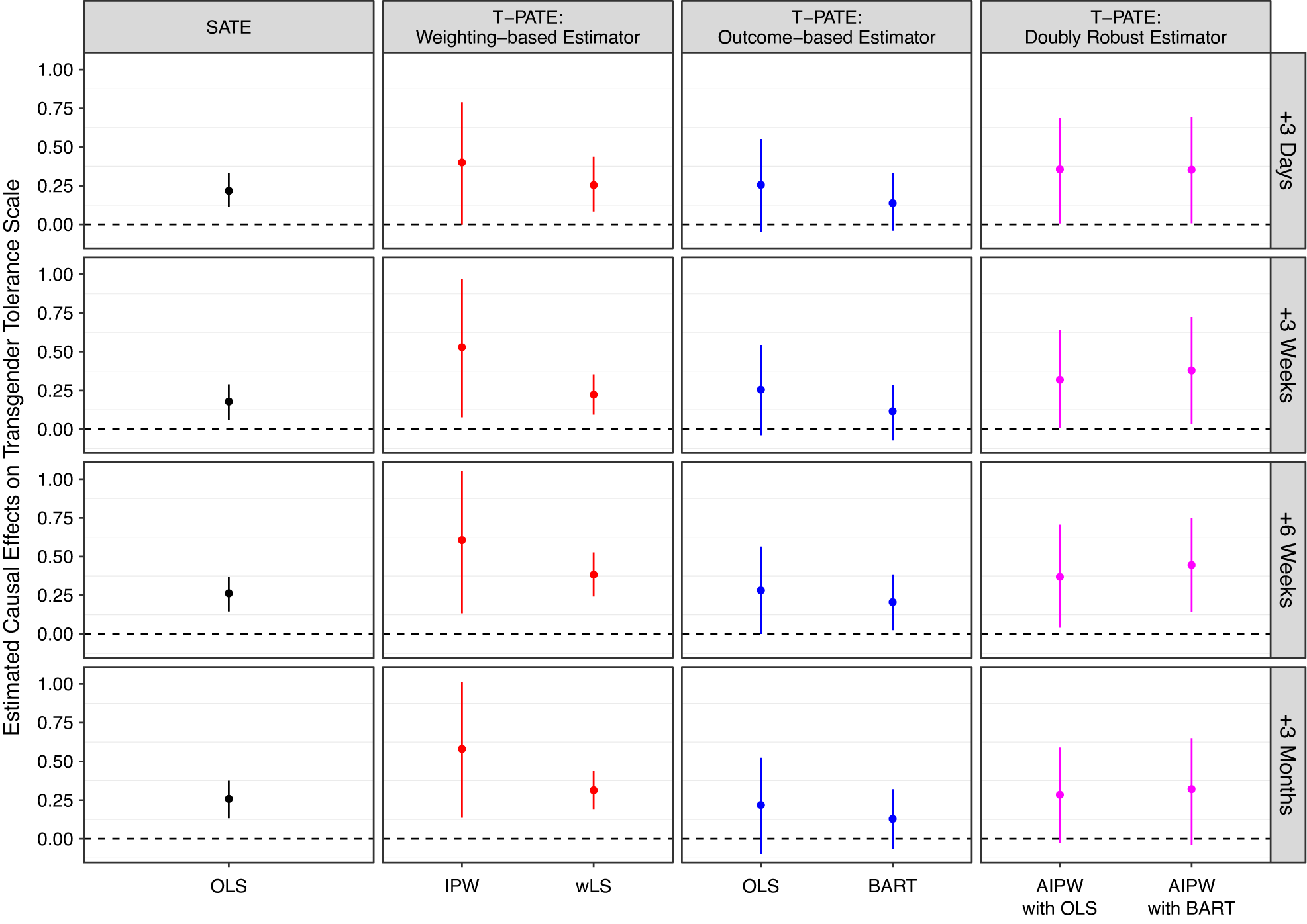

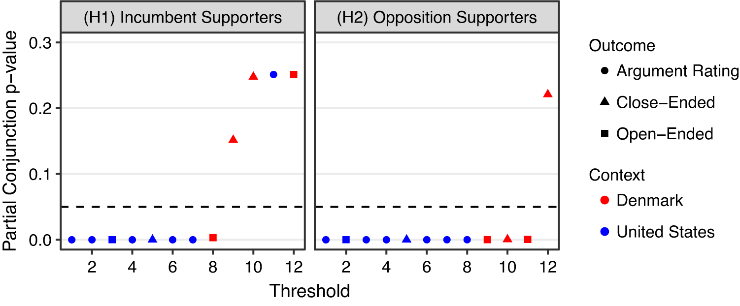


 Open access
Comments
No Comments have been published for this article.