


1. Introduction
In boreal and Arctic lakes, when the air temperature drops below freezing point in early winter, lake water releases heat to the atmosphere, usually resulting in columnar ice formation. However, if there is a lot of turbulence in the lake water, granular ice may sometimes be formed initially, but the dominating mechanism for granular ice formation is snow-to-ice transformation. The ice layer acts as an effective insulator between the lake water and atmosphere (Leppäranta, Reference Leppäranta and George2010). Changes of climate conditions at high latitudes affect the lake ice season, resulting in a number of feedbacks on the regional climate in the winter-spring season (Brown and Duguay, Reference Brown and Duguay2010).
Finland is a boreal country with tens of thousands of lakes that freeze every winter. Snowfall is guaranteed in Finnish Lapland in every winter season. Snow cover affects lake ice physics, mass balance and phenology (Leppäranta, Reference Leppäranta2015). A striking phenomenon is the snow-to-ice transformation. In cold conditions, a heavy snowpack pushes columnar ice below the water surface, resulting in a negative freeboard and formation of slush and refreezes to snow-ice (Leppäranta, Reference Leppäranta1983; Eicken and others, Reference Eicken, Fischer and Lemke1995; Rösel and others, Reference Rösel2018). The formation of snow ice is very important for the radiation attenuation through the snow-covered ice layer (Lei and other, Reference Lei, Leppäranta, Erm, Jaatinen and Pärn2011). In spring, meltwater from snow or rainfall may percolate downwards and refreeze to superimposed ice at the snow/ice interface (Kawamura and others, Reference Kawamura, Ohshima, Takizawa and Ushio1997; Nicolaus and others, Reference Nicolaus, Haas and Bareiss2003; Granskog and others, Reference Granskog, Vihma, Pirazzini and Cheng2006). Therefore, snow-to-ice transformation results in granular ice formation, and the growth of the ice layer from the snow/ice interface upwards. This is different from the columnar ice growth downwards from the ice bottom.
Meteorological conditions are the primary driving force for the evolution of snow depth and ice thickness in Arctic lakes (Wei and others, Reference Wei2016). However, in the case of large lakes, the existence of lake ice provides feedback to local meteorological conditions, in particular, the presence of lake ice strongly reduces surface evaporation and, hence, also the occurrence and amount of precipitation (Wright and other, Reference Wright, Posselt and Steiner2013). To better understand the impact of lake ice on climate, we need sustainable long-term measurements of snow depth and ice thickness in frozen lakes. An array of stakes and thickness gauges or borehole measurements are the easiest way to measure ablation and accumulation snow and lake ice thickness. Challenges remain in obtaining sustainable snow and ice thickness measurements in remote areas, as long-term manned observations for cryo limnology are very expensive to maintain.
Autonomous snow and ice mass-balance buoys (IMB) are widely used (Perovich and Elder, Reference Perovich and Elder2001). Some IMBs apply Acoustic Rangefinder Sounders (ARS) mounted above and below the snow surface and ice bottom. ARS measure the distances from the sensor in the air downward to the snow surface and from the sensor in the sea upward to the ice bottom. Using the initial snow/ice interface as a fixed reference level, one can easily convert ARS data to obtain snow accumulation and melt, ice surface ablation, as well as ice bottom growth and ablation, and finally the time series of snow depth and ice thickness (Richter-Menge and others, Reference Richter-Menge, Perovich, Elder and Claffey2006). The ARS-IMB is a powerful and effective instrument largely used to monitor snow and ice mass balance in the Polar Oceans (Perovich and Elder, Reference Perovich and Elder2001, Polashenski and others, Reference Polashenski, Perovich and Courville2012). The ARS sensors have also been used to detect ice surface erosion for a high-mountain lake due to strong sublimation (Huang and others, Reference Huang2016). For a high-mountain lake, ARS can accurately detect the entire snow and ice thickness as a whole.
In boreal lakes, ice is often thinner than that in the Arctic Ocean. A heavy snowfall on a thin ice layer may result in slush formation at the snow/ice interface and later in refreezing to snow-ice. In addition, the snowmeltwater, sleet and rain may refreeze to form superimposed ice at the snow/ice interface. Hence, the snow/ice interface is a dynamic moving boundary between the snow and lake ice (Cheng and others, Reference Cheng2014). For Polar Oceans, the formation of snow ice or superimposed ice is also prevailing for the seasonal sea ice in the Antarctic (Fichefet and Morales Maqueda, Reference Fichefet and Morales Maqueda1999), Arctic (Granskog and others, Reference Granskog2017; Rösel and others, Reference Rösel2018), and the Baltic Sea (Granskog and others, Reference Granskog, Martma and Vaikmäe2003). Temperature measurements can also be used to distinguish snow/sea/ice interface. For example, snow-ice formation observed in the Arctic winter has resulted in snow/ice interface moving upward (Provost and other, Reference Provost2017, Reference Provost, Sennéchael and Sirven2019).
One of the temperature-based IMBs (T-IMB) is called the High-resolution Snow and Ice Mass-Balance Array (SIMBA; Jackson and others, Reference Jackson2013) that has been developed by the Scottish Association for Marine Science (SAMS) Research Services Ltd (SRSL). SIMBA measures the environment temperature (SIMBA-ET) using a 4.8-m-long thermistor string with sensors spaced at 2 cm intervals. The sensors are numbered from the top (1) in the air to the lowermost (240) in the water. The SIMBA-ET is typically recorded 4 times a day. In addition, SIMBA measures the heating temperature (SIMBA-HT) applying a small identical heating element on each sensor. The heating is applied once per day. The heating interval usually lasts for 60 s or 120 s. The temperature changes in air, snow, ice and water are different due to the different heat conductivities. The heating temperature can be used to identify interfaces among the air-snow-ice-water system. Compared with the ARS-IMB, the SIMBA-IMB has a lower cost, allowing deployment in large numbers, for example, across the Arctic Ocean. This reduces the risk of loss of the buoys due to sea-ice fragmentation (Thompson and others, Reference Thompson, Jackson and Cheng2019). SIMBA data have been used for snow depth and ice thickness monitoring and energy-balance studies in a seasonally ice-covered lake (Cheng and others, Reference Cheng2014) and for the Polar Oceans (Hoppmann and others, Reference Hoppmann2015; Provost and others, Reference Provost2017; Reference Provost, Sennéchael and Sirven2019; Lei and others, Reference Lei2018). For the Polar environment, T-IMB has difficulties to identify interfaces during summer when snow layer and ice floe are likely isothermal vertically.
A SIMBA-algorithm was developed by Liao and others (Reference Liao2018) and are used to extract snow depth and ice thickness from SIMBA-ET data. The algorithm was targeted for SIMBA data obtained from the Arctic Ocean, where the snow/ice interface remained unchanged. Retrieval of snow depth and ice thickness from SIMBA data from lakes has so far been a manual process (Cheng and others, Reference Cheng2014). Hence, it is necessary to develop a method to process lake SIMBA data systematically to minimize the uncertainties of a manual process and keep the results consistent.
This study focused on lake ice. The SIMBA-algorithm was adapted for lakes. The new threshold values of temperature changes were defined based on SIMBA-ET data analyses. The SIMBA-algorithm was first developed and validated using SIMBA and in situ snow and ice measurements made on Lake Orajärvi, northern Finland in winter 2011/12. Then we applied the algorithm to investigate SIMBA measurements for winters 2017/18 and 2018/19. Our objectives are to assess the applicability of the modified SIMBA-algorithm for lake ice data analyses, in particular for the detection of moving snow/ice interface, and for analyses of the snow-to-ice transformation. Compared with the Arctic Ocean conditions, the SIMBA lake ice measurements are facing a temporal variation of snow/ice interface.
2. Observations and methodology
2.1 Lake site
A SIMBA buoy was deployed in Lake Orajärvi (Fig. 1), which is a typical boreal mid-size lake with a surface area of ~11 km2 and a mean water depth of 4.4 m. The ice season typically starts in mid- or late-November and lasts until early- or mid-May. The observed maximum ice thickness is often up to 70 cm in late April before the melt onset (Cheng and others, Reference Cheng2014). The first snowfall typically occurs in late October, but the snow may melt during warmer autumn days. The seasonally permanent winter snow accumulation usually starts between mid-November and early-December.
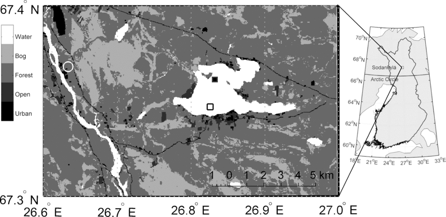
Fig. 1. Map of Lake Orajärvi, where the open black square marks the SIMBA site in winters 2017/18 and 2018/19, where the water depth was 5.2 m and the white circle marks the Sodankylä weather station, 10 km east from the lake, at the Finnish Meteorological Institute (FMI) Arctic Space Centre (http://fmiarc.fmi.fi/) (ARC) 120 km north of the Arctic Circle. The filled black square ■ was the SIMBA site for 2011/12 winter season.
2.2 Weather station
The automatic weather station (AWS, WMO code 02836) was located 10 km from Lake Orajärvi at FMI ARC main camp. The AWS records air temperature (PT100 sensor), wind speed (Vaisala WAA25), humidity (Vaisala HMP) and cloudiness (Vaisala CT25K). Precipitation intensity (mm/h) was measured by Vaisala FD12P sensor and precipitation amount (mm) by Ott Messtechnik Pluvio2 weighting gauge. The snow depth was obtained by Campbell Scientific SR50 sensor. The solar shortwave radiative flux (Kipp&Zonen CM11: 305–2800 nm) and thermal longwave radiative flux (Kipp&Zonen CG4: 4500–42 000 nm) were measured 40 m from the AWS in a tower with unobstructed sky view. All measurements were made once a minute. The data have been post-processed to create time series of hourly and daily means.
2.3 Method and validation
The SIMBA-algorithm (Liao and others, Reference Liao2018) is based on continuity of heat flux in the vertical direction from the ice base to the snow surface. The differences between heat conductivities of snow and sea ice as well as the resolution of temperature sensors were taken into account to construct the algorithm. Consistency of the entire snowpack and sea-ice column is assumed, i.e. the effects of firm snow layer (a very thin layer of ice within the snowpack, formed via refreezing of percolated liquid water), snow-ice, superimposed ice, as well as snow and sea-ice internal melting on SIMBA-ET changes, were not considered. In this study, a modified interface identification procedure is developed.
The temperature profiles in air and water are assumed as isothermal above the snow surface and below ice bottom. The lake ice bottom was identified according to the freezing temperature (0°C). In a shallow lake, the bottom water temperature is often well above the freezing temperature (Leppäranta, Reference Leppäranta2015). A stratified interfacial layer often prevails just beneath the ice bottom with a clearly distinguishable temperature gradient (Huang and others, Reference Huang2019). We introduced a concept called SIMBA-ET Temperature Minimum Resolution Criteria (TMRC). Because the resolution of SIMBA temperature sensors was ± 0.0625°C (defined as ΔT), we assume −0.0625°C as the freezing temperature at the ice bottom, i.e. at an interface of solid ice and liquid water. Any temperature changes <0.5 × |0.0625| °C was regarded as no change. We, therefore, applied a threshold range from [-0.0625-|ΔT| to 0.0625 + |ΔT|] oC to identify the ice bottom position. We scanned thermistor string readings from the bottom sensor upwards, and the sensor number that gave the temperature readings with this threshold range was identified as the ice bottom zone. The average position of the ice bottom zone was defined as the ice bottom.
The snow surface identification is adapted from the original SIMBA-algorithm. It is largely based on the difference between the spatial temperature gradient in air and snow. The first-order derivative (FOD) of air temperature in a fixed vertical distance of 2 cm is assumed to be very small since the near-surface air temperature is almost constant in height. To detect the snow surface, we calculated SIMBA-ET FOD (in °C m−1) from the top sensor downwards. The FOD of temperature would have increased abruptly when the thermistor sensor was placed from air into the snowpack. Once the snow surface position was identified, the snow/ice interface is identified from the sensors located between snow surface and ice bottom only.
The identification of the snow/ice interface was carried out by calculating the second-order derivative (SOD) of the SIMBA-ET in space (2 cm). Because of the heat conductivity, density and heat capacity of snow and ice are different, the vertical temperature profile is nonlinear in snow and quasi-linear in lake ice. The SOD of ET value in the ice layer should be 0°C m−2. In practice, however, the calculated SOD slightly deviated from zero. The calculated SOD in the snow layer (with a small heat conductivity and density) showed a sinusoidal pattern in response to rapid temperature changes at the snow surface. Due to thermal inertia, the signal attenuated further down into the snowpack. At the snow/ice interface, interactions, including phase changes, are visible when looking at SOD values. Based on changes of SIMBA-ET criteria used in the original SIMBA-algorithm and the SOD calculation, we used the value of 2 × ΔT °C m−2 = 0.125 °C m−2 of SIMBA-ET SOD to identify the snow/ice interface, The 0.125 ± ΔT °C m−2 was used as a threshold range, i.e. [0.0625, 01875] °C m−2 to define the uncertainty of snow/ice interface. Similar to the treatment of the ice bottom, the average position identified by the threshold range was defined as the snow/ice interface. We note that when we calculate the FOD and SOD, we refer to the values that cross a fixed spatial interval of 2 cm. We are interested in the spatial temperature change within this spatial interval (FOD) and the changes of FOD in the same spatial interval.
Validation was carried out applying SIMBA ET time series for 2011/12 season where biweekly borehole snow depth and ice thickness measurements were available. A manual process was applied to identify snow depth and ice thickness (Cheng and others, Reference Cheng2014) based on visual inspection of vertical SIMBA-ET profiles on a weekly basis. The interfaces and thicknesses detected by the method presented above and by manual process are shown in Figure 2. A 5-point moving average was applied to the algorithm identified interfaces to remove unrealistic spikes from the results.
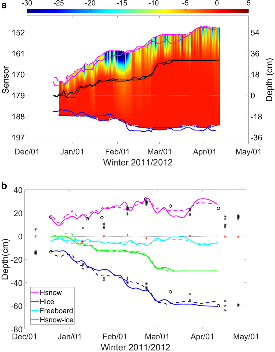
Fig. 2. (a) SIMBA-ET temperature profile for 2011/12 ice season. The Lagrangian (here defined as positions of all interfaces are moving corresponding to its previous positions) evolution of snow surface, snow/ice interface and ice bottom are marked as magenta, black and blue lines, respectively. The thin white line is the initial snow/ice interface at the time of SIMBA deployment. For better clarity, the temperature profile above the snow surface and the below ice bottom by the manual process was removed. (b) Snow depth (magenta) and total ice thickness (blue) using the snow/ice interface (black lines in plot a) as the zero reference level. The time series of snow-ice thickness is represented by the difference between the zero reference level and the location of the initial snow/ice interface (thin white line in a). The ice freeboard (cyan) is calculated on the basis of Eqn (1). The asterisks and circles are in situ snow and ice thicknesses measurements in the lake at observation sites apart 500 m from each other. The solid lines are obtained by the method presented above and dashed lines are results from the manual process (Cheng and other, 2014).
According to the Archimedes' principle, the ice freeboard (fb) can be calculated based on time series of snow depth (hs), snow-ice thickness (Hsi) and columnar ice thickness (Hi):

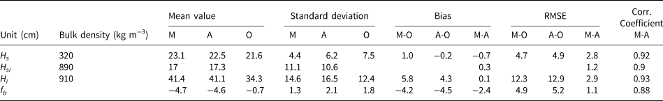
where ρs, ρsi and ρi are seasonal mean densities of snow, snow-ice and columnar ice, respectively (Table 1). The snow depth, ice freeboard, snow-ice and total ice thickness based on manual process and algorithm-based calculations are close to each other (Table 1).
Table 1. Comparisons between manual (M) /algorithm (A) derived and observed snow depth (Hs), snow-ice (Hsi) and total ice thickness (Hi) as well as the statistical calculation of Bias, (RMSE and correlation coefficient between manual (M)/algorithm (A) calculated and observed (O) and, manual (M) and algorithm (A)-derived results
Both air/snow and snow/ice interfaces move upward in response to snowfall and snow-to-ice transformation, respectively. The ice/water interface move downwards as a result of bottom freeze-up. A 57 cm ice block sample was collected on 12 April 2012, when the SIMBA was recovered. It was composed of 24 cm (42%) columnar ice and 33 cm (58%) granular snow-ice and superimposed ice (Cheng and others, Reference Cheng2014). Compared to 14 cm initial ice thickness when SIMBA was deployed on 19 December 2011, the net ice bottom growth was 10 cm, in agreement with SIMBA detection. Most of the ice growth occurred at the snow/ice interface.
3. Result and discussion
A SIMBA was configured to measure SIMBA-ET vertically at the UTC times of 23:00, 05:00, 11:00 and 17:00, and at 00:00, 06:00, 12:00 and 18:00 UTC for winter 2017/18 and 2018/19, respectively. The heating element was activated right after the 11:00 UTC for 2017/18 and 06:00 UTC for 2018/19. The SIMBA-HT was obtained after the heating periods of 60 and 120 s were recorded.
3.1 Ice season 2017/2018
3.1.1 Deployment
A SIMBA buoy was deployed on 15 December 2017. At the time of deployment, the air temperature was −7°C, snow depth was 40 cm on land, and 35–30 cm on lake ice near the shore. At the SIMBA deployment site, some 700 m from the shore (Fig. 1), total snow depth of 25 cm was composed of 18 cm of soft snow and 7 cm of hard snow. The snow load had caused lake water flooding on top of the ice, generating a 5–6 cm slush layer within the lowermost parts of the snowpack. When a borehole was drilled, it triggered heavy flooding up to 10–11 cm above the ice surface (Fig. 3a). The ice thickness was 23 cm. On 3 May 2018, SIMBA was recovered. At the time, no snow was seen on the lake ice surface (Fig. 3b). The air temperature was +3°C and snow thickness on land was 40 cm. On lake ice, in addition to snowdrift, sublimation and evaporation, a large part of snow layer was transferred to granular ice. The total ice thickness was 55 ± 2 cm at the SIMBA site. The ± 2 cm represents the measurement uncertainty due to the softness and rotten characteristic of the granular ice surface. Compared to the initial ice surface in December, the ice had grown upwards. There was 19 ± 1 cm snow-ice on top at the time when we recovered the thermistor chain (Fig. 4). The ice layer marked in the scale between 13.5 and 22 cm in Fig. 4 had a crystal structure of snow-ice, probably formed via refreezing of slush in early winter prior to the SIMBA deployment. The ice layer marked in the scale between 22 and 37 cm showed a crystal structure resembling columnar ice. However, this ice layer cannot have been formed via freezing of lake water because it was placed above the snow-ice layer that was formed at the snow/ice interface. A possible explanation could be that when the borehole was drilled, we removed the snow (Fig. 4)and the flooded water layer eventually froze up to form columnar ice, and afterwards, a second layer of snow-ice was formed on top in cold conditions. The ice bottom melt occurred already when SIMBA was recovered (see 3.1.2).
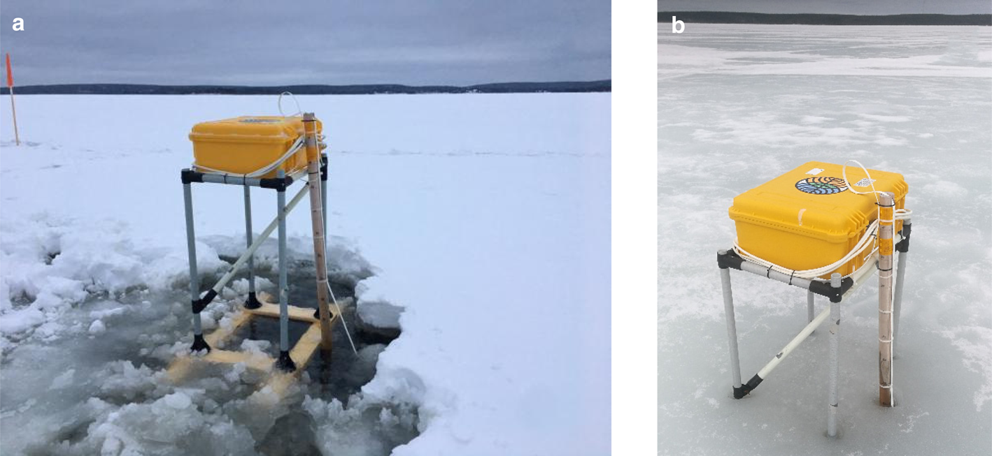
Fig. 3. The SIMBA site (67.35° N, 26.83° E) on the deployment day of 15 December 2017 (a) and the recovery day of 2 May 2018 (b). The freezing of ice above the original snow/ice interface was evident.
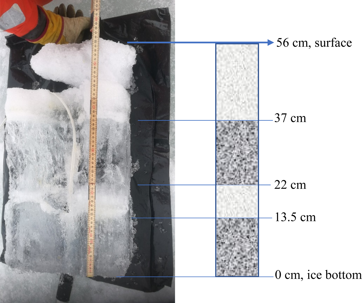
Fig. 4. An ice block picked up on 3 May 2018, in order to recover SIMBA thermistor chain. The composition of the ice block is schematically illustrated on the right side. The dark grey sections represent columnar ice whereas the light grey sections indicate granular ice.
3.1.2 SIMBA temperature profiles, snow depth and ice thickness
SIMBA-ET and SIMBA-HT profiles are illustrated in Figure 5. For better clarity, we plot the temperature only between sensors 70 and 150, as the changes of interfaces occurred within this 160 cm layer. The evolution of the ice bottom was ± 6 cm (between sensors 125 and 130). The ice base was initially located between sensors 128 and 129. Before recovering SIMBA, sensor 100 was at the ice surface and the total ice thickness was 55 cm. Accordingly, the ice bottom was located between sensors 127 and 128. The change of the ice bottom remained small due to (a) the strong insulation by the thick snowpack and (b) the compensating effects of pronounced ice growth in February and melt from late April onwards.
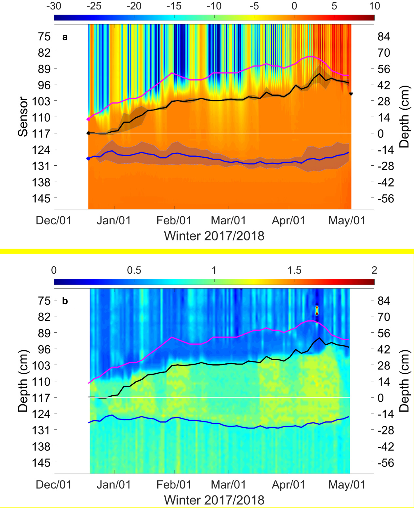
Fig. 5. (a) Evolution of air/snow (magenta), snow/ice (black) and ice/water (blue) interfaces. The asterisks (*) represent sensor positions for the snow and ice surface when SIMBA was deployed and for the ice surface when SIMBA was recovered. The background colour is the SIMBA-ET temperature profile measured between sensors 70 and 150. The white line was the initial snow/ice interface. The shadow belts represent the uncertainties of snow/ice and ice/water interfaces. (b) Time series of SIMBA-HT ratio (HT60/HT120). The lines are the same as in (a).
The SIMBA-HT ratio revealed two distinguishable interfaces (Fig. 5b). These were located very close to the snow/ice interface and, in particular, the ice bottom was detected by SIMBA-ET. Unfortunately, we do not have in situ snow and ice measurements to validate the seasonal evolution of the snow/ice interface and ice bottom, except the borehole measurements during the deployment and recovery stages. The snow/ice interface and ice bottom evolution may be somehow reflected by the SIMBA-HT ratio. For example, the steady strong SIMBA-HT ratio in December and early January may represent a freezing process of the flooded water layer.
The snow/ice interface rose 52 cm upwards from sensor 117 to sensor 91. When the SIMBA was deployed, snow was removed around the borehole and a layer of 10–11 cm flooded water exposed on top of ice layer. This layer froze gradually making snow/ice interface moved upward. Snow/ice interface remained almost the same from mid-February to early March (Fig. 5b). During this period, snow depth on land remained quite the same (Fig. 6).
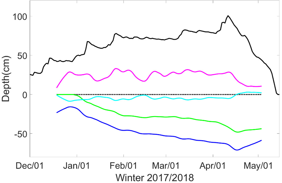
Fig. 6. Time series of snow accumulation on land (black) and on lake ice (magenta) using snow/ice interface (black line in Fig. 5) as the zero reference level, thickness of granular ice (green) due to formation of snow-ice or superimposed ice; calculated freeboard (cyan), and the total thickness of granular and columnar ice (blue).
After the deployment, the ice bottom zone was ~20 cm thick (sensors 120–130) until the end of February. In March and early April, the zone got thinner (~10 cm) before it became thicker again from early April onwards. The exact reason for such a large uncertainty on the location of the ice bottom remained unknown. A possible explanation could be that after the deployment the thermistor string lying in the ice borehole was submerged below the flooded water all the way from surface down to the ice bottom and the vertical temperature gradient remained small before the borehole and flooded water above refroze up entirely. In Arctic deployments, the freeze-up of ice borehole may take up to 1 month (Liao and others, Reference Liao2018). In April, melt could start at the ice bottom resulting in a weak vertical temperature gradient at the lower part of the ice layer enhancing the uncertainty of ice bottom interface detection. For the snow/ice interface zone, the threshold value range did not yield a large uncertainty, except in early January and mid-April. Looking at the time series of snow accumulation on land, an abrupt increase of snowfall was observed in January, and rapid snowmelt occurred in mid-April. These events could trigger slush formation at snow/ice interface due to flooding or snow melting.
The time series of snow depth, freeboard and ice thickness (Fig. 6) demonstrate that snow contributed to the total ice thickness. During most of the ice season, heavy snow resulted in a negative freeboard to form granular ice. The seasonal mean snow-ice thickness was 27 cm, which was 54% of the mean total ice thickness. The maximum ice thickness was 71 cm on 16 April 2018. The mean snow depth was 24 cm during SIMBA observation period (13 December–2 May). During the same period, the mean snow thickness at Sodankylä snow station on land was 69 cm, i.e. 2.9 times larger than on lake ice.
3.2 2018/19
3.2.1 Deployment
For winter 2018/19, a SIMBA buoy was deployed on 13 December (Fig. 7a) 2018 approximate at the same location as in the previous year. The air temperature was −23°C on 12 December and raised to −9°C when we deployed the SIMBA. Snow depth on land had remained thin until early December. The lake ice was formed in almost snow-free conditions, until major snowfall events occurred on 3 and 7 December. The snow depth on land was 20 cm, as it was also on lake ice near the shore. The snow depth slightly reduced, to 18–19 cm, towards the SIMBA site, where the lake ice thickness was 14–15 cm. A 2 cm of flooding was observed when the borehole was drilled but it was rapidly refrozen because of the cold air temperature. SIMBA was recovered on 2 May 2019, when snow was still seen on the ice surface, but it was under a melting phase with a very inhomogeneous distribution (Fig. 7b). The total ice thickness was 55 ± 1 cm, of which columnar ice, snow-ice and superimposed ice contributed 22, 25.5 and 7.5 cm, respectively. The measurement uncertainty at surface was ±1 cm, (Fig. 8)

Fig. 7. SIMBA site (67.35°N, 26.86°E) on deployment day 13 December 2018 in (a) and recover day 2 May 2019 in (b).
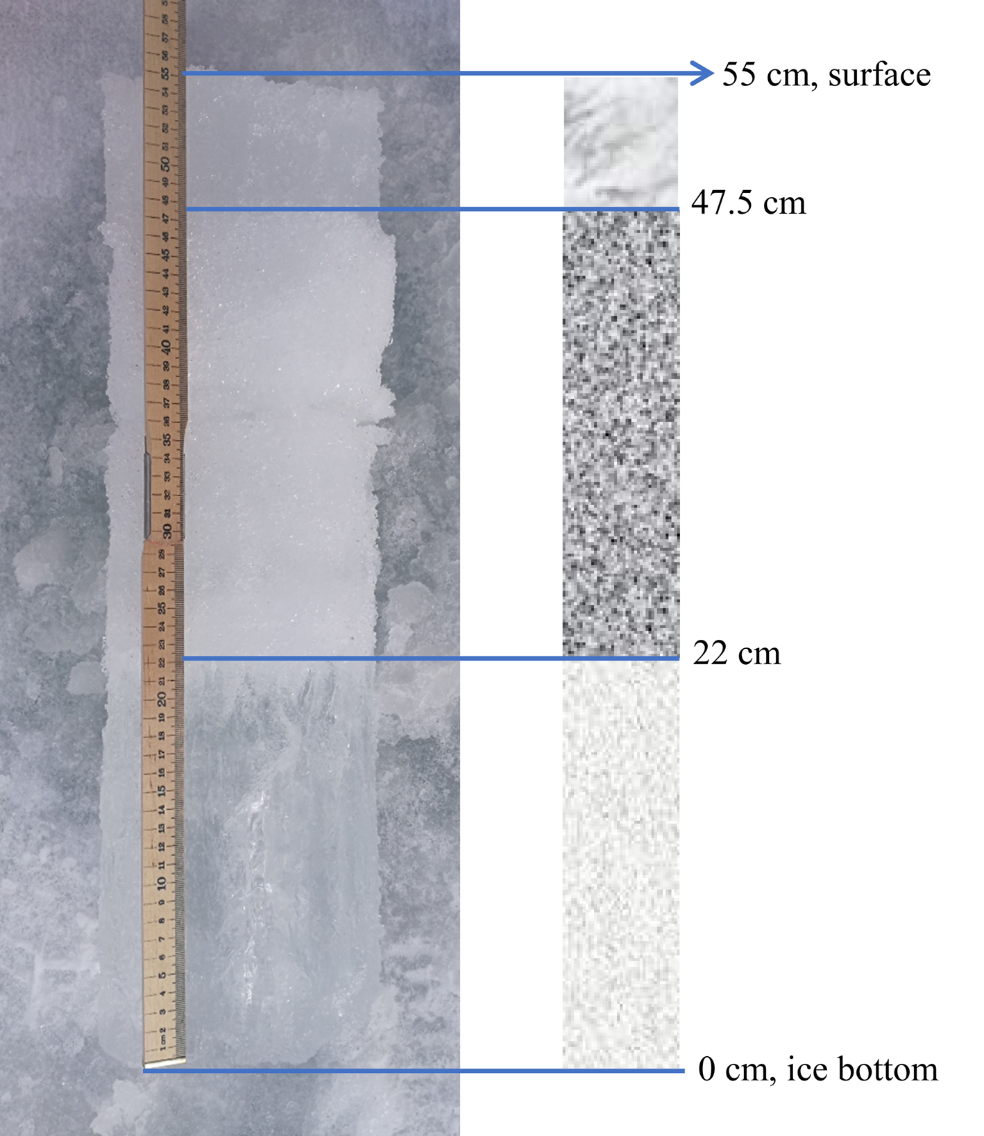
Fig. 8. Ice block sample collected on 3 May 2018 5 m away from the SIMBA deployment site.
3.2.2 SIMBA temperature profiles, snow depth and ice thickness
For 2018/19 winter season, the maximum snow accumulation on land was about the same as in the previous winter, but the precipitation pattern was different. Snow started to accumulate some 10 d before SIMBA deployment (Fig. 9) and air temperature was cold before and after SIMBA deployment. SIMBA-ET revealed some 20 cm basal ice growth in December and January (between sensors 125 and 135; Fig. 10a). The bottom growth is not significant from February to early April. The ice bottom began to melt in mid-April.
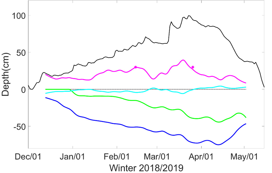
Fig. 9. Same as Figure 5, but for 2018/2019 ice season.
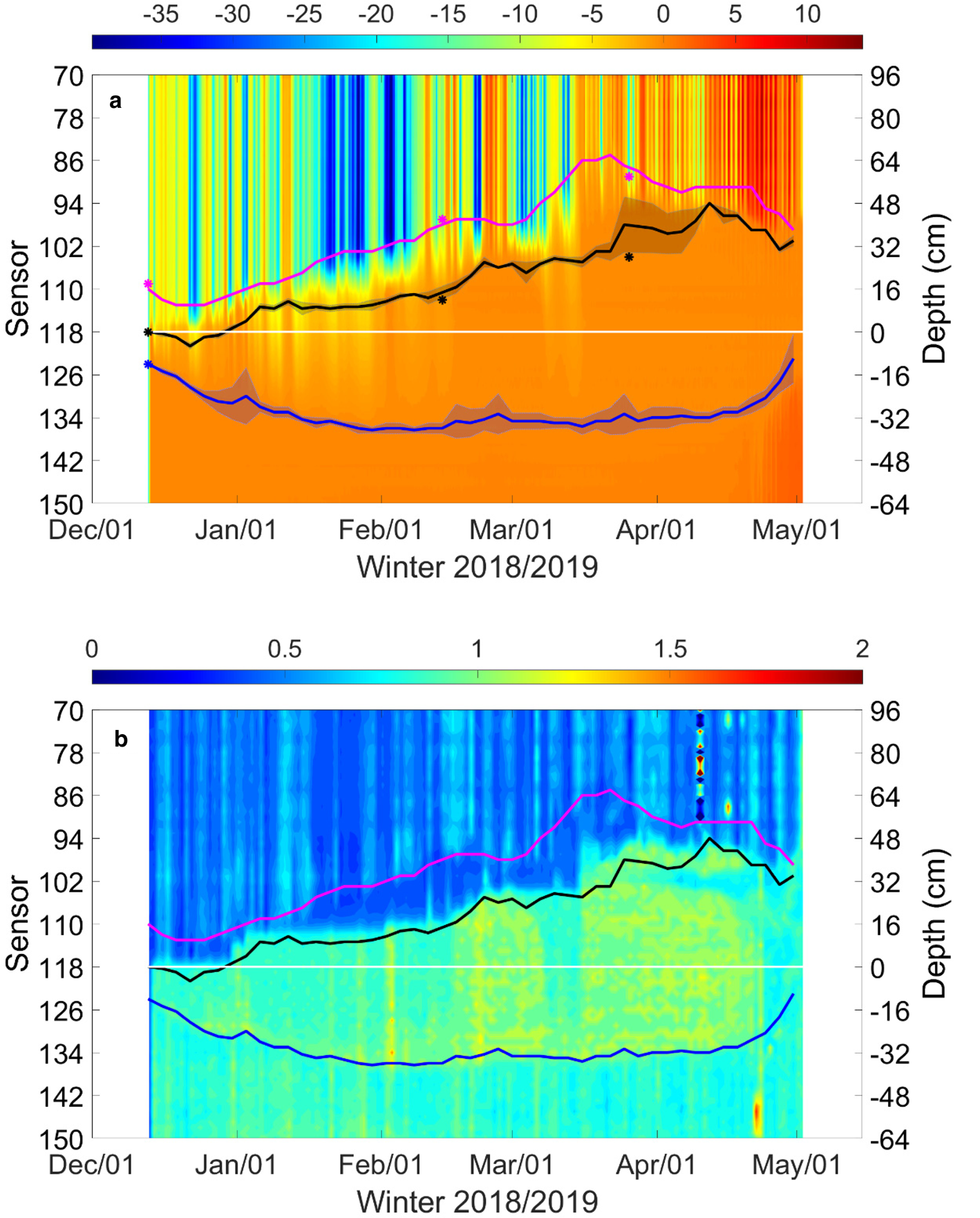
Fig. 10. Time series of snow accumulation on land (black), on lake ice (magenta) using snow/ice interface (black line in Fig. 9) as the zero reference level, thickness of granular ice (green) due to formation of snow-ice or superimposed ice; calculated freeboard (cyan), and the total thickness of granular and columnar ice (blue).
Snow accumulation was substantial. The initial snow surface moved up from its original position (sensor 117) at frozen floodwater surface on 14 December, to the top position some 64 cm higher (sensor 85) in mid-March. The corresponding snow/ice interface evolved from sensor 117 to sensor 94 in mid-April moving up 46 cm in total. From December to late March, the position of snow/ice interface moved up gradually consistent with the increase of snow depth on land. The overall ice bottom zone was confined to a thin layer. During early January, late February and late March, the uncertainties of ice bottom detection were getting large probably in response to air temperature increase and large precipitation. The ice bottom position (Fig. 10 blue line) was in good agreement with that identified based on SIMBA-HT. In late March and early April, the snow/ice interface showed a large range of variety which was linked with snowmelt onset. The seasonal mean snow-ice thickness was 21 cm, which was 41% of the mean total ice thickness. The maximum ice thickness was 75 cm on 12 April 2019. Snow on land was 2.7 times thicker than on lake ice, i.e., the ratio was almost the same as in 2017/18. The SIMBA-HT (Fig. 10b) showed similar characteristics, i.e. two discriminate interfaces that were close to the SIMBA-ET-based snow-ice and ice/water interfaces. The SIMBA-HT at the ice bottom well matched the ice bottom derived from SIMBA-ET.
3.3 Discussion
The time series of meteorological parameters observed for both ice seasons are given in Figure 11, and monthly and seasonal mean values are summarized in Table 2. During the observation periods, the accumulated freezing degree day (FDD) was 1617°C for 2017/18 and 1425°C for 2018/19. On the basis of air temperature alone, one would expect thicker ice for season 2017/18. The SIMBA-ET, however, suggested a larger maximum ice thickness of 75 cm for 2018/19 compared to 71 cm for 2017/18. The difference could be explained by the snow conditions. The seasonal mean snow depth on land was 50 cm for 2017/18 and 40 cm for 2018/19. The corresponding numbers for the SIMBA observation periods were 69 and 49 cm, respectively. A thicker snowpack yields a stronger insulation effect and reduces/increases columnar/granular ice formation. During the observation period in the lake, the mean snow depth/ice thickness was 24/48 cm for 2017/18 and 21/51 cm for 2018/19. The corresponding mean granular/columnar ice thickness was 27/21 cm for 2017/18 and 21/30 cm for 2018/19. When SIMBA was recovered on 3 May for both seasons, the ice thicknesses were almost the same. However, the compositions of ice columns were different, and the differences can largely be explained by the different seasonal patterns of air temperature and precipitation. The coldest month was February for 2017/18 with a mean air temperature of −14.9°C, whereas for 2018/19, the coldest month was January with a mean air temperature of −16.8°C.
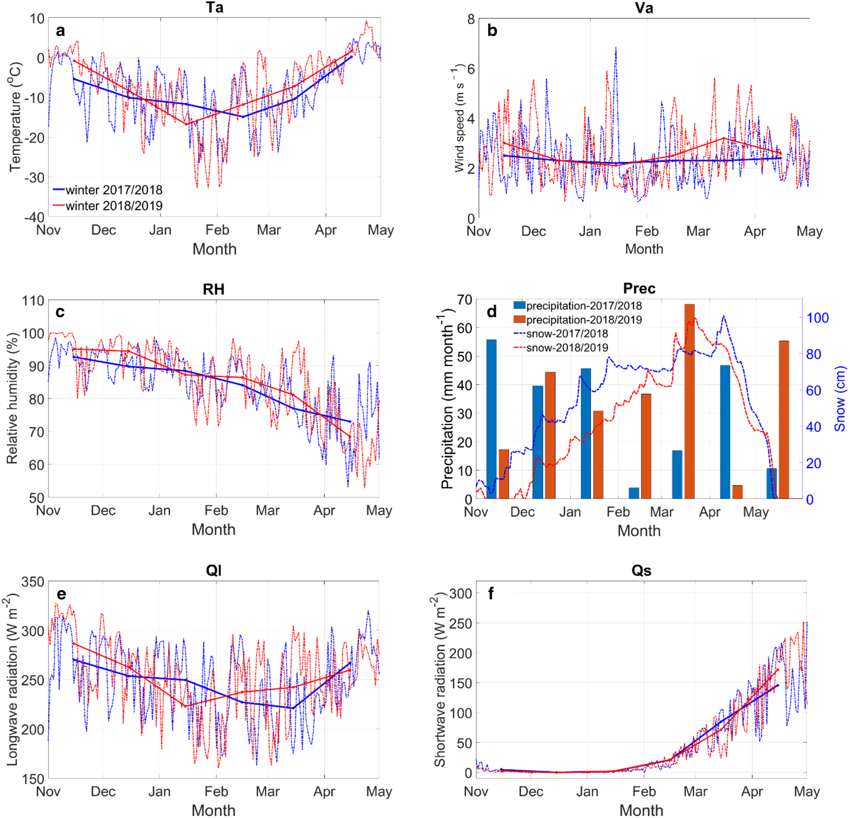
Fig. 11. Monthly (solid line) and daily (dashed line) mean values of (a) air temperature (T a), (b) wind speed (V a), (c) relative humidity (RH), (d) monthly accumulated precipitation (P rec), (e) downward longwave radiative flux (Q l), and (f) downward shortwave radiative flux (Q s) observed at Sodankylä weather station for 2017/18 (blue) and 2018/19 (red) ice seasons.
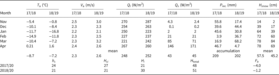
Table 2. Monthly mean air temperature (T a), wind speed (V a), downward longwave (Q l) and shortwave (Q s) radiative fluxes, monthly accumulated precipitation (P rec), mean snow thickness (H snow) on land as well as lake snow depth (hs), snow-ice (Hsi), columnar ice (Hi), total ice thickness (H total) and ice freeboard (Fb)
The accumulated precipitation was close to each other for both ice seasons (November–April), but the accumulation pattern (snow thickness) was different. Snow started to accumulate on land in late October 2017 and stayed permanently until snowmelt started on 10 April 2018. For 2018/19, the first snowfall occurred in early October but melted away until the permanent seasonal snow accumulated in mid-December. Snowmelt started on 22 March 2019. A heavy snowfall in early winter combined with a low air temperature is favourable for more granular ice and less columnar ice formation. The different monthly and seasonal mean wind speeds also contributed to the difference of snow accumulation patterns between the seasons. In both ice seasons, the monthly mean relative humidity was high in winter and gradually reduced towards spring. The monthly mean pattern of downward longwave radiative fluxes was like that of the air temperatures. The accumulated thawing degree-days (TDD) during the observation period was 45°C and 119°C for 2017/18 and 2018/19, respectively. The corresponding numbers for April were 39°C and 81°C. The higher number in April for 2018/19 was partly contributed by more available shortwave solar radiation.
The validation results for the calculated of freeboard were poor (Table 1). Ice freeboard is a function of snow and ice thickness and density (Eqn 1). Compared with a relatively constant lake ice density, the seasonal snow density may range from150 to 450 kgm−3 (Barrere and others, Reference Barrere, Domine, Decharme, Morin, Vionnet and Lafaysse2017). Figure 12 shows the sensitivity of the calculated freeboard to the seasonal mean snow density for 2011/12 winter. The sensitivity increases with a thicker snowpack (Fig 12a). On a seasonal scale, the negative freeboard linearly increases with increasing snow density (Fig 12b). Accurate calculation of ice freeboard is still a challenge.

Fig. 12. (a) Time series of calculated freeboard for 2011/12 assuming a seasonal mean snow density of 250, 300, 320 and 400 kg m−3. The red circles mark the observed freeboard and the vertical bars denote its standard deviation. (b) Relationship between calculated seasonal mean freeboard and snow density. The coloured circles mark calculations for different seasons.
5. Conclusions
A thermistor-string-based ice mass-balance buoy (SIMBA) was deployed in Lake Orajärvi in northern Finland to monitor vertical temperature profiles through air/snow/ice/water column during 2017/18 and 2018/19 ice seasons. The vertical profiles of environment temperature (ET) and heating temperature (HT) were measured with a resolution of 2 cm using temperature sensors with a resolution of ± 0.0625°C. The SIMBA-ET data were used to retrieve the snow depth and lake ice thickness based on a method adapted from the original SIMBA-algorithm (Liao and others, Reference Liao2018). The first-order derivative (FOD) and second-order derivative (SOD) of the SIMBA-ET temperature profile, as well as the TMRC, are control factors in our method to identify the air/snow, snow/ice and ice/water interfaces. The TMRC threshold criteria used in this study worked well to identify the interfaces. The SIMBA-ET retrieved snow depth and ice thickness were in good agreement with the manual SIMBA data process. Both results were comparable to the borehole snow and ice measurements.
Two SIMBA-IMBs were successfully deployed on Lake Orajärvi ice in winter seasons 2017/18 and 2018/19. The snow accumulation was large in these two winters. The total observed precipitation during the winter season (November–April) was 209 mm for 2017/18 and 202 mm for 2018/19. The heavy snowfall in early winter 2017/18 triggered considerable flooding on lake ice. Snow-ice formation was evidently lifting the snow/ice interface during the winter. During both winters, snow-ice formation contributed largely to the ice growth on Lake Orajärvi. The seasonal mean snow-ice thickness was 40–55% of the mean total ice thickness. The evolution of the snow/ice interface was primarily consistent with the change of snow surface. The mean snow depth on lake ice was 35–37% of that on land nearby, which is somewhat less than observed for a lake in southern Finland (44% by Kärkäs (Reference Kärkäs2000)). The heavy snowfall yields negative freeboard that is linearly inversely proportional to the snow density. However, the calculation of ice freeboard based on SIMBA buoy data requires further improvement.
The method used in this study only applied the SIMBA-ET profile, which includes sufficient information to identify air/snow/ice/water interfaces. The SIMBA-HT profiles were solely used to compare and validate interfaces that were derived from SIMBA-ET. The SIMBA-HT ratio profile showed discrete interfaces, which were very close to the snow/ice interface and ice bottom detected based on the time series of the SIMBA-ET profiles. The comparisons between different ratios of SIMBA-HT profile can qualitatively differentiate snow thermal properties (Gani and others, Reference Gani, Sirven, Sennéchael and Provost2019). The seasonal differences of SIMBA-HT between 2017/18 and 2018/19 were small. For a given time step, the larger SIMBA-HT ratio at the surface was associated with newly fallen snow, which usually has a small heat conductivity and density. SIMBA-HT profiles are potentially useful to differentiate the thermal diffusivities of air, snow, ice and water and further the interfaces between those media.
The operational monitoring of snow and ice thickness in boreal lakes is still mostly a manual process (e.g. Lei and others, Reference Lei, Leppäranta, Cheng, Heil and Li2012). The method developed in this study was applicable to retrieve snow depth and ice thickness from SIMBA IMBs deployed in the boreal lake. The use of SIMBA as a primary tool for lake snow and ice measurements would be very cost-effective. The other type thermistor-string units has been developed and used for operational monitoring of river ice (Deng and others, Reference Deng2020). The cost-cutting design of the T-IMB makes it possible to carry out coordinated deployments over a large region to investigate spatial variations and regional means of snow and ice mass balance. The algorithm developed in this study will be a useful tool for interpretation of SIMBA data both observed in boreal lakes and Polar Oceans. However, for Polar Oceans, the snow and ice are close to isothermal during summer, which prevents identification of interfaces on the basis of the temperature gradient. Under such conditions, thermodynamic modelling yields valuable information on snow depth and ice thickness (Tian and others, Reference Tian2017).
Acknowledgement
The study was for financial support by the National Key R&D Program of China (Grant No. 2016YFC1402705); The Chinese Scholarship Council (No. 201904910510); The European Union's Horizon 2020 research and innovation programme [727890 – INTAROS]; Academy of Finland under contract 317999; The National Natural Science Foundation of China (41922044, 11571383); The Fundamental Research Funds for the Central Universities (grant no. 19lgzd07); the Key Research Program of Frontier Sciences of CAS (QYZDY-SSW-DQC021) and the Guangdong Basic and Applied Basic Research Foundation (No. 2020B1515020025). We are grateful to Mr. Pekka Kosloff for carrying out fieldwork in Lake Orajärvi for all the winter seasons since 2009. We are grateful for comments by several anonymous reviewers and scientific editor Dr David Babb, which helped to improve the manuscript significantly.


 Open access